
Locate hidden cells
Follow these steps:
-
Select the worksheet containing the hidden rows and columns that you need to locate, then access the Special feature with one of the following ways:
-
Press F5 > Special.
-
Press Ctrl+G > Special.
-
Or on the Home tab, in the Editing group, click Find & Select>Go To Special.
-
-
Under Select, click Visible cells only, and then click OK.

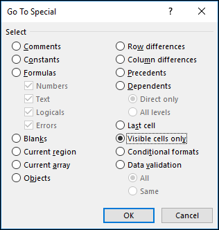
All visible cells are selected and the borders of rows and columns that are adjacent to hidden rows and columns will appear with a white border.
Note: Click anywhere on the worksheet to cancel the selection of the visible cells. If the hidden cells that you need to reveal are outside the visible worksheet area, use the scroll bars to move through the document until the hidden rows and columns that contain those cells are visible.
This feature is not available in Excel for the web.
Содержание
- Процедура включения отображения
- Способ 1: размыкание границ
- Способ 2: Разгруппировка
- Способ 3: снятие фильтра
- Способ 4: форматирование
- Вопросы и ответы

При работе с таблицами Excel иногда нужно скрыть формулы или временно ненужные данные, чтобы они не мешали. Но рано или поздно наступает момент, когда требуется скорректировать формулу, или информация, которая содержится в скрытых ячейках, пользователю вдруг понадобилась. Вот тогда и становится актуальным вопрос, как отобразить скрытые элементы. Давайте выясним, как можно решить данную задачу.
Процедура включения отображения
Сразу нужно сказать, что выбор варианта включения отображения скрытых элементов в первую очередь зависит от того, каким образом они были скрыты. Зачастую эти способы используют совершенно разную технологию. Существуют такие варианты скрыть содержимое листа:
- сдвиг границ столбцов или строк, в том числе через контекстное меню или кнопку на ленте;
- группирование данных;
- фильтрация;
- скрытие содержимого ячеек.
А теперь попробуем разобраться, как можно отобразить содержимое элементов, скрытых при помощи вышеперечисленных методов.
Способ 1: размыкание границ
Чаще всего пользователи прячут столбцы и строки, смыкая их границы. Если границы были сдвинуты очень плотно, то потом трудно зацепиться за край, чтобы раздвинуть их обратно. Выясним, как это можно сделать легко и быстро.
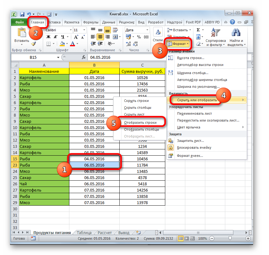
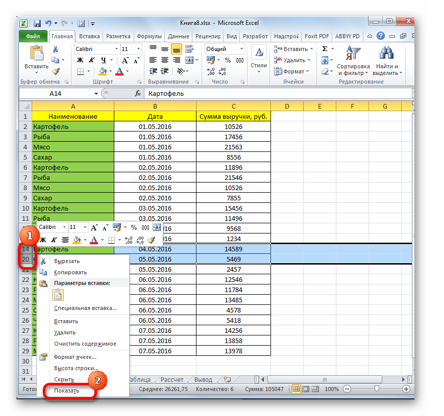
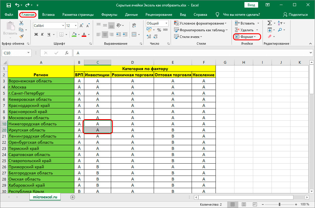
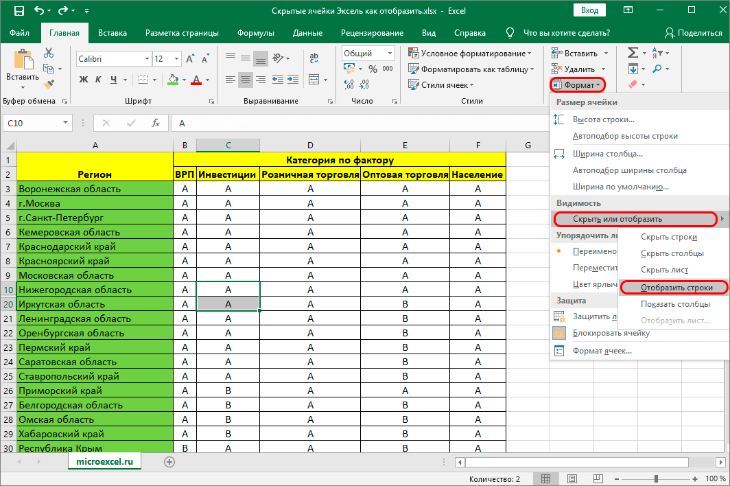
- Выделяем две смежные ячейки, между которыми находятся скрытые столбцы или строки. Переходим во вкладку «Главная». Кликаем по кнопке «Формат», которая расположена в блоке инструментов «Ячейки». В появившемся списке наводим курсор на пункт «Скрыть или отобразить», который находится в группе «Видимость». Далее в появившемся меню выбираем пункт «Отобразить строки» или «Отобразить столбцы», в зависимости от того, что именно скрыто.
- После этого действия скрытые элементы покажутся на листе.
Существует ещё один вариант, который можно задействовать для отображения скрытых при помощи сдвига границ элементов.
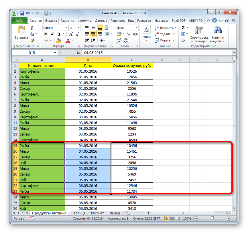
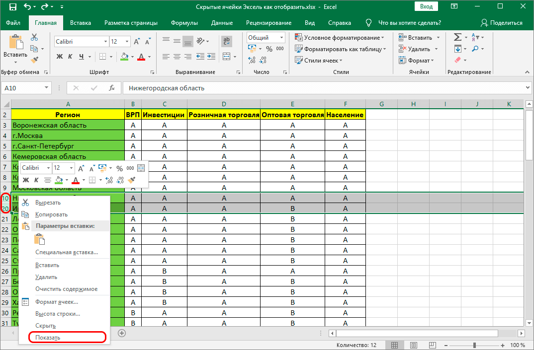
- На горизонтальной или вертикальной панели координат, в зависимости от того, что скрыто, столбцы или строки, курсором с зажатой левой кнопкой мыши выделяем два смежных сектора, между которыми спрятаны элементы. Кликаем по выделению правой кнопкой мыши. В контекстном меню выбираем пункт «Показать».
- Скрытые элементы будут тут же отображены на экране.
Эти два варианта можно применять не только, если границы ячейки были сдвинуты вручную, но также, если они были спрятаны с помощью инструментов на ленте или контекстного меню.
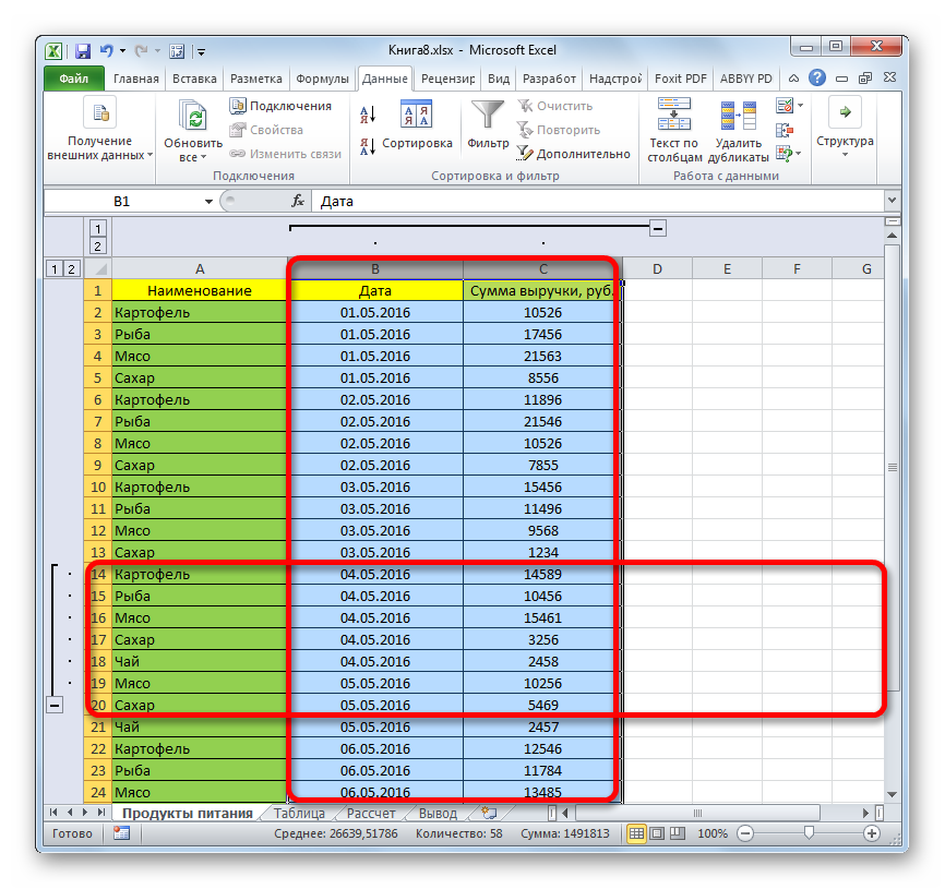
Способ 2: Разгруппировка
Строки и столбцы можно также спрятать, используя группировку, когда они собираются в отдельные группы, а затем скрываются. Посмотрим, как их отобразить на экране заново.
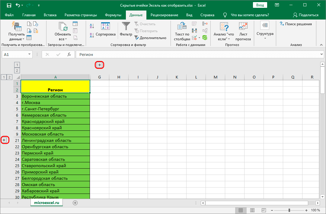
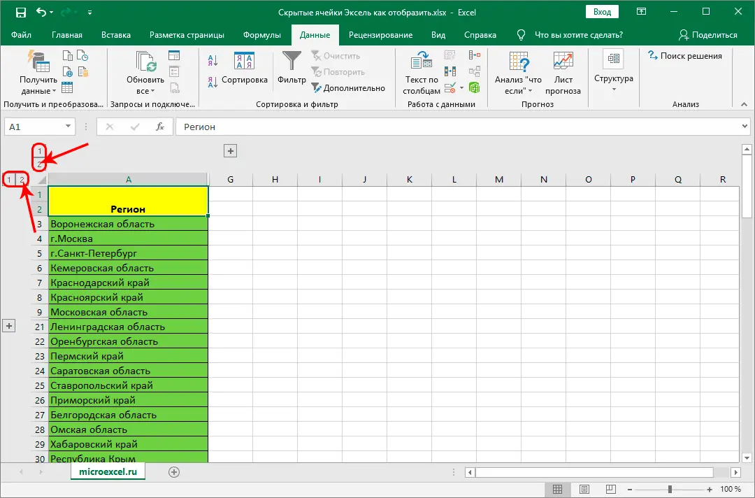
- Показателем того, что строки или столбцы сгруппированы и спрятаны, является наличие значка «+» слева от вертикальной панели координат или сверху от горизонтальной панели соответственно. Для того, чтобы показать скрытые элементы, достаточно нажать на этот значок.

Также можно их отобразить, нажав на последнюю цифру нумерации групп. То есть, если последней цифрой является «2», то жмите на неё, если «3», то кликайте по данной цифре. Конкретное число зависит от того, сколько групп вложено друг в друга. Эти цифры расположены сверху от горизонтальной панели координат или слева от вертикальной.
- После любого из данных действий содержимое группы раскроется.
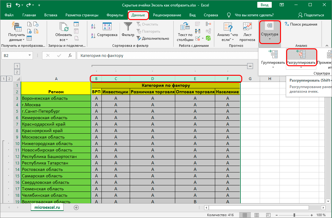
- Если же для вас этого недостаточно и нужно произвести полную разгруппировку, то сначала выделите соответствующие столбцы или строки. Затем, находясь во вкладке «Данные», кликните по кнопке «Разгруппировать», которая расположена в блоке «Структура» на ленте. В качестве альтернативного варианта можно нажать комбинацию горячих кнопок Shift+Alt+стрелка влево.


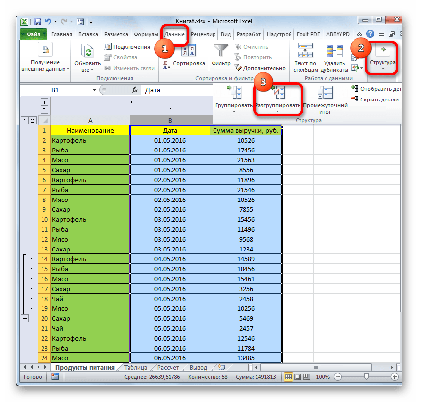

Группы будут удалены.
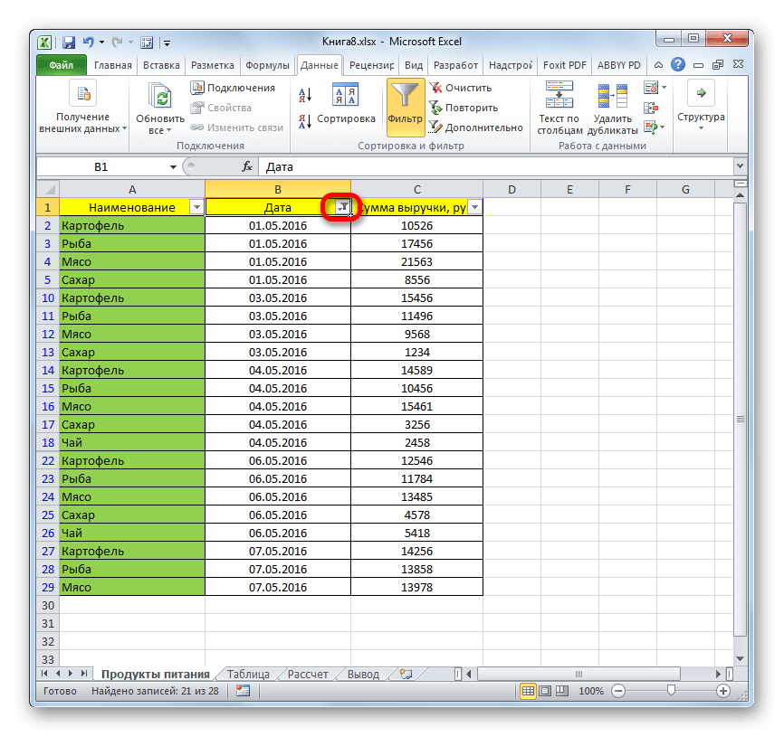
Способ 3: снятие фильтра
Для того, чтобы скрыть временно ненужные данные, часто применяют фильтрацию. Но, когда наступает необходимость вернуться к работе с этой информацией, фильтр нужно снять.
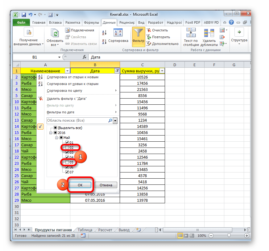
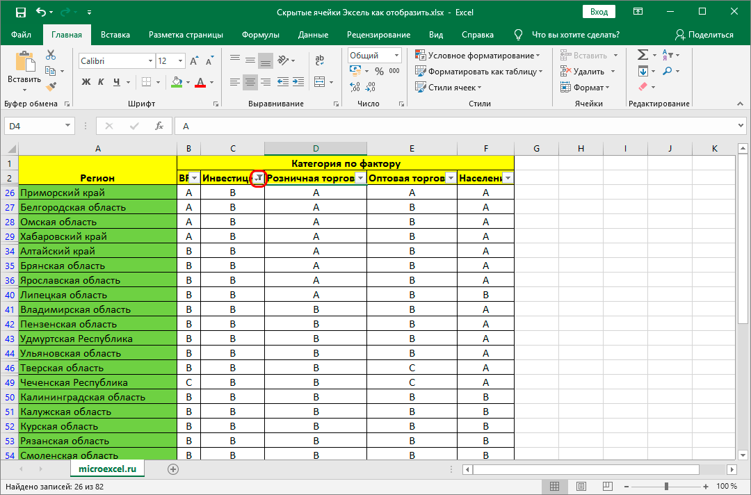
- Щелкаем по значку фильтра в столбце, по значениям которого производилась фильтрация. Такие столбцы найти легко, так как у них обычная иконка фильтра с перевернутым треугольником дополнена ещё пиктограммой в виде лейки.
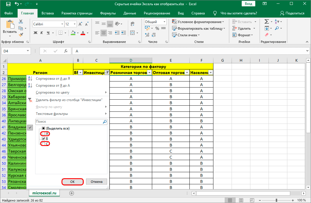
- Открывается меню фильтрации. Устанавливаем галочки напротив тех пунктов, где они отсутствуют. Именно эти строки не отображаются на листе. Затем кликаем по кнопке «OK».
- После этого действия строки появятся, но если вы хотите вообще удалить фильтрацию, то нужно нажать на кнопку «Фильтр», которая расположена во вкладке «Данные» на ленте в группе «Сортировка и фильтр».

Способ 4: форматирование
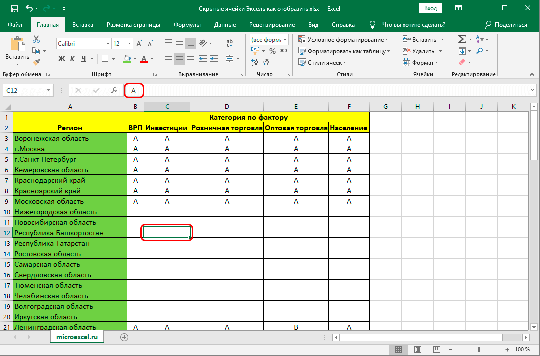
Для того чтобы скрыть содержимое отдельных ячеек применяют форматирование, вводя в поле типа формата выражение «;;;». Чтобы показать спрятанное содержимое, нужно вернуть этим элементам исходный формат.
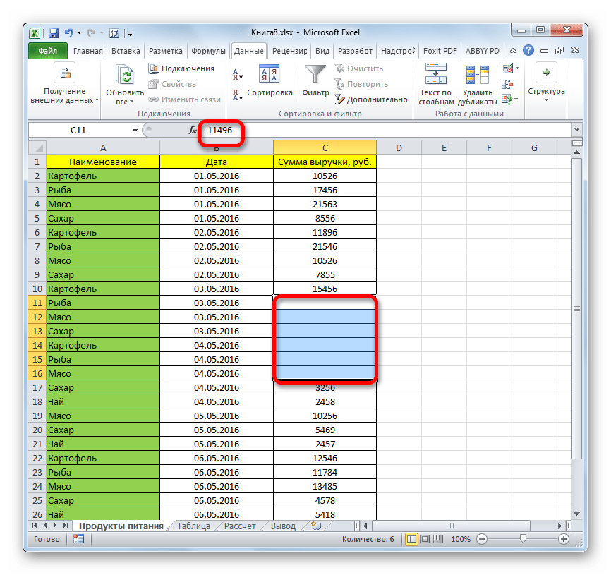
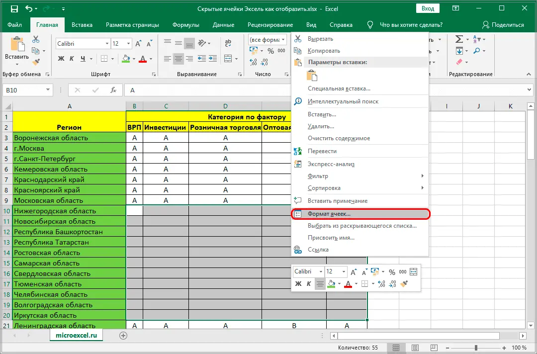
- Выделяем ячейки, в которых находится скрытое содержимое. Такие элементы можно определить по тому, что в самих ячейках не отображается никаких данных, но при их выделении содержимое будет показано в строке формул.
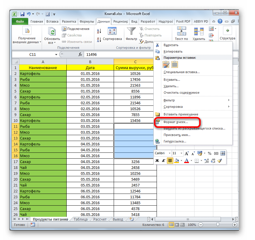
- После того, как выделение было произведено, кликаем по нему правой кнопкой мыши. Запускается контекстное меню. Выбираем пункт «Формат ячеек…», щелкнув по нему.
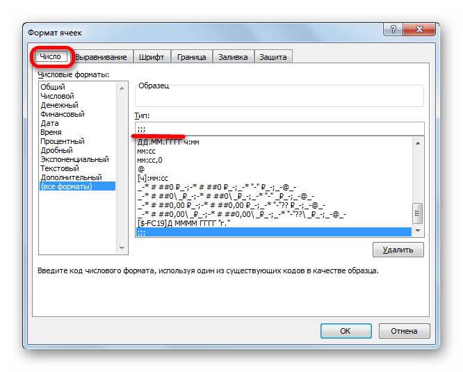
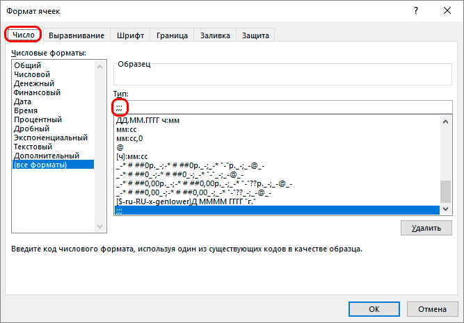
- Запускается окно форматирования. Производим перемещение во вкладку «Число». Как видим, в поле «Тип» отображается значение «;;;».
- Очень хорошо, если вы помните, каково было изначальное форматирование ячеек. В таком случае вам только останется в блоке параметров «Числовые форматы» выделить соответствующий пункт. Если же вы не помните точного формата, то опирайтесь на сущность контента, который размещен в ячейке. Например, если там находится информация о времени или дате, то выбирайте пункт «Время» или «Дата», и т.п. Но для большинства типов контента подойдет пункт «Общий». Делаем выбор и жмем на кнопку «OK».
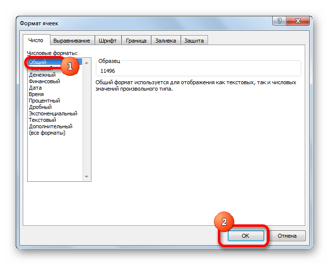
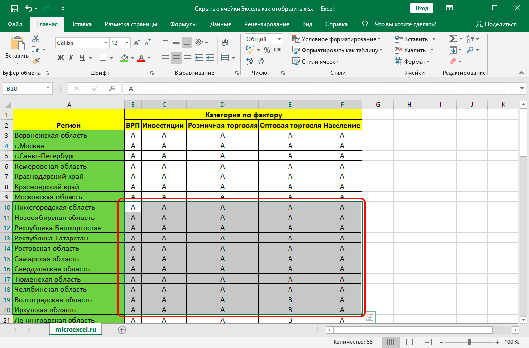
Как видим, после этого скрытые значения снова отображаются на листе. Если вы посчитаете, что отображение информации некорректно, и, например, вместо даты видите обычный набор цифр, то попробуйте ещё раз поменять формат.

Урок: Как изменить формат ячейки в Excel
При решении проблемы отображения скрытых элементов главная задача состоит в том, чтобы определить, с помощью какой технологии они были спрятаны. Потом, исходя из этого, применять один из тех четырех способов, которые были описаны выше. Нужно уяснить, что если, например, контент был скрыт путем смыкания границ, то разгруппировка или снятие фильтра отобразить данные не помогут.
When working with different tables in Excel format, sooner or later it will be necessary to temporarily hide some data or hide intermediate calculations and formulas. At the same time, deletion is unacceptable, since it is possible that editing of hidden data will be required to get the formulas to work correctly. To temporarily hide this or that information, there is such a function as hiding cells.
How to hide cells in Excel?
There are several ways to hide cells in Excel documents:
- changing the boundaries of a column or row;
- using the toolbar;
- using the quick menu;
- grouping;
- enable filters;
- hiding information and values in cells.
Each of these methods has its own characteristics:
- For example, hiding cells by changing their borders is the easiest. To do this, just move the cursor to the bottom border of the line in the numbering field and drag it up until the borders touch.
- In order for hidden cells to be marked with “+”, you need to use the “Grouping”, which can be found in the “Data” menu tab. Hidden cells will thus be marked with a scale and a “-” sign, when clicked, the cells are hidden and a “+” sign appears.
Important! Using the “Grouping” option, you can hide an unlimited number of columns and rows in the table
- If necessary, you can also hide the selected area through the pop-up menu when you press the right mouse button. Here we select the item “Hide”. As a result, the cells disappear.
- You can hide several columns or rows through the “Home” tab. To do this, go to the “Format” parameter and select the “Hide or show” category. Another menu will appear, in which we select the necessary action:
- hide columns;
- hide lines;
- hide sheet.
- Using the filtering method, you can hide information in several rows or columns at the same time. On the “Main” tab, select the “Sort and Filter” category. Now in the menu that appears, activate the “Filter” button. A checkbox with an arrow pointing down should appear in the selected cell. When you click on this arrow in the drop-down menu, uncheck the boxes next to the values uXNUMXbuXNUMXbthat you want to hide.
- In Excel, it is possible to hide cells without values, but at the same time not violate the structure of calculations. To do this, use the “Cell Format” setting. To quickly call up this menu, just press the combination “Ctrl + 1”. On the left side of the window, go to the “(all formats)” category, and in the “Type” field, go down to the last value, that is, “;;;”. After clicking on the “OK” button, the value in the cell will disappear. This method allows you to hide some values, but all formulas will work properly.
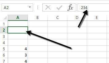
Search for hidden cells
If several users are working on a document, then you should know how to detect the presence of hidden cells in an Excel file. To only find hidden columns and rows, but not display them, you will have to check the sequence of all column and row headings. A missing letter or number indicates hidden cells.
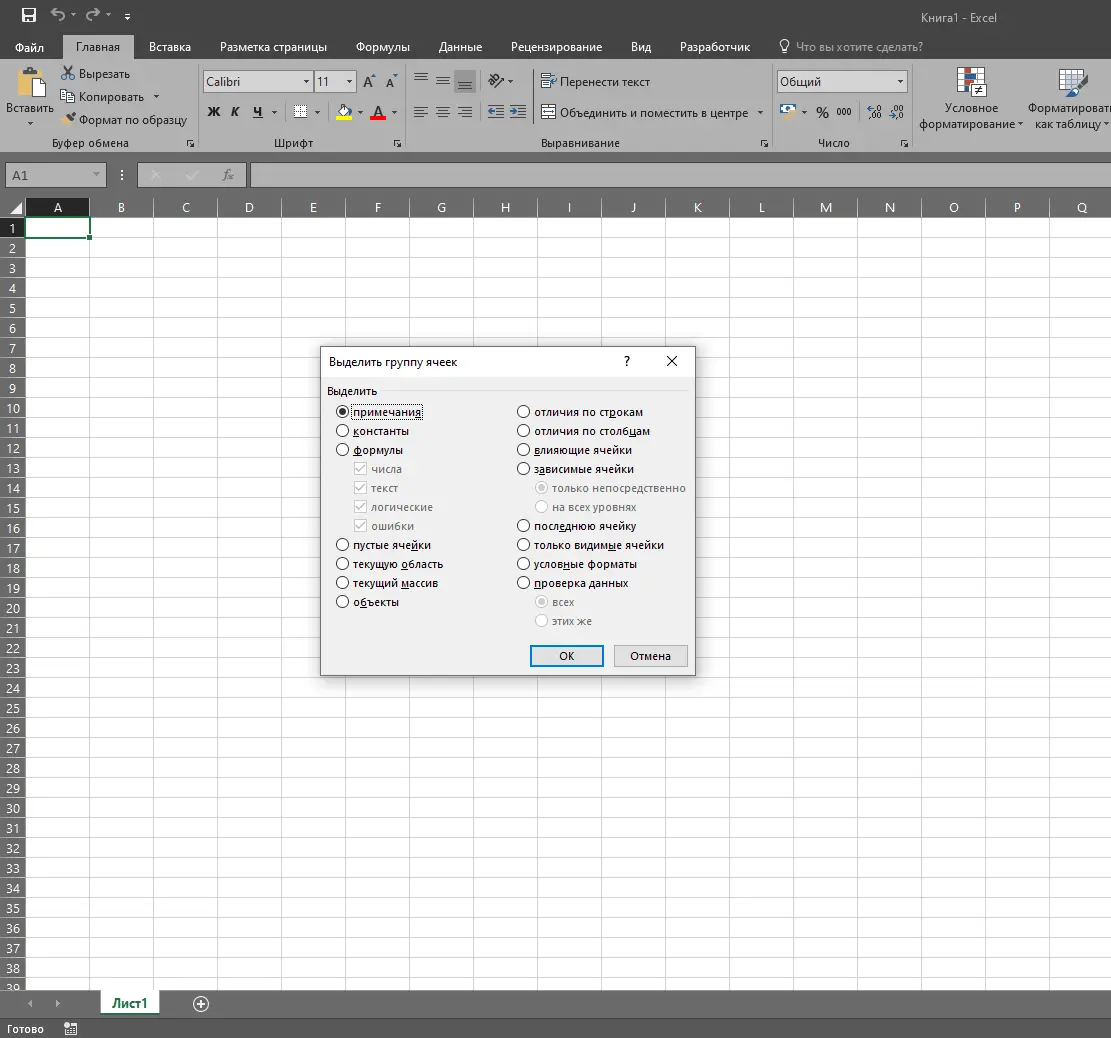
If the table is too large, then this method is extremely inconvenient. To simplify the process of finding hidden cells in a document, you need to go to the “Editing” command set in the “Home” menu. In the “Find and select” category, select the “Select a group of cells …” command.
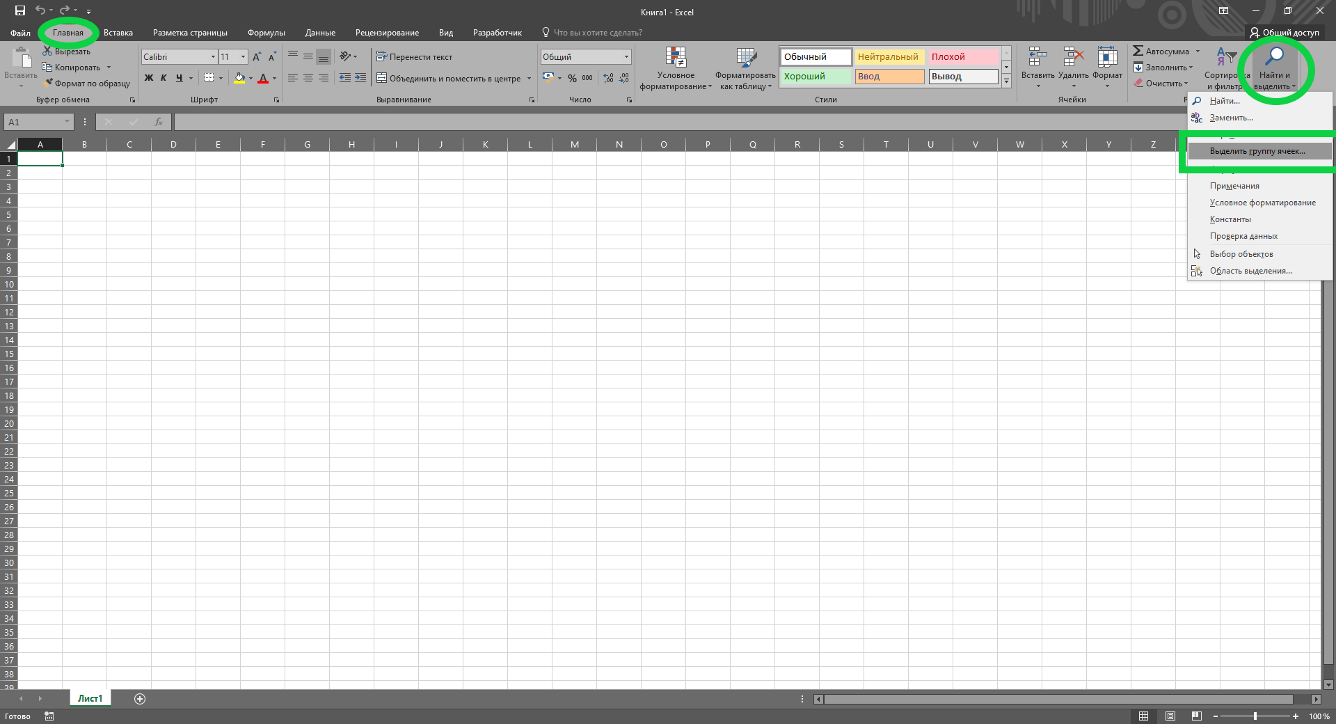
In the window that opens, check the “Only visible cells” category. After that, within the table, you can see not only the selected area of cells, but also thickened lines, which indicate the presence of hidden rows or columns.
Show hidden cells in Excel
Just like that, opening cells hidden from prying eyes will not work. First you need to understand the methods that were used to hide them. After all, the choice of their display will depend on this. For example, these could be:
- displacement of cell borders;
- ungrouping of cells;
- turning off the filter;
- formatting certain cells.
Let us consider each of them in more detail.
Method 1: Shift Cell Borders
If the method of physically shifting the boundaries of a column or line was used to hide cells, then to display it is enough to return the boundaries to their original position using a computer mouse. But you should carefully control every movement of the cursor. And in the case of a large number of hidden cells, their display can take quite a long time. But even this task can be done in a matter of seconds:
- It is necessary to select two adjacent cells, and there must be a hidden cell between the cells. Then in the “Cells” toolbox in the “Home” menu we find the “Format” parameter.
- When you activate this button in the pop-up menu, go to the “Hide or show” category. Next, select one of the functions – “Display Rows” or “Display Columns”. The choice depends on which cells are hidden. At this point, the hidden cells will be displayed immediately.
Advice! In fact, this rather simple method can be further simplified, and most importantly, accelerated. To begin with, we select not only adjacent cells, but adjacent rows or columns, between which By clicking on the right button of the computer mouse, a pop-up menu will appear, in which we select the “Show” parameter. Hidden cells will appear in their place and will be editable.
These two methods will help to reveal and display hidden data only in case of manual hiding of cells in the Excel spreadsheet.
Method 2: Ungroup Cells
An Excel tool called grouping allows you to hide a specific area of cells by grouping them together. Hidden data can be shown and hidden again using special keyboard shortcuts.
- First, we check the Excel sheet for hidden information cells. If there are any, then a plus sign will appear to the left of the line or above the column. When you click on the “+” all grouped cells will open.
- You can reveal hidden areas of a file in another way. In the same area where the “+” is, there are also numbers. Here you should select the maximum value. The cells will be displayed when you click on the number with the left mouse button.
- In addition to temporary measures for displaying cells, grouping can be turned off completely. We select a specific group of rows or columns. Next, in the tab called “Data” in the “Structure” tool block, select the “Ungroup” category.
- To quickly remove a grouping, use the keyboard shortcut Alt+Shift+Left Arrow.
Method 3: Turn off the filter
One powerful way to find and organize large amounts of information is to filter table values. It should be borne in mind that when using this method, some columns in the file table go into hidden mode. Let’s get acquainted with the display of hidden cells in this way step by step:
- Select a column filtered by a specific parameter. If the filter is active, then it is indicated by a funnel label, which is located next to the arrow in the top cell of the column.
- When you click on the “funnel” of the filter, a window with available filter settings will appear. To display hidden data, tick each value or you can activate the “Select All” option. Click “OK” to complete all settings.
- When filtering is cancelled, all hidden areas in the Excel spreadsheet will be displayed.
Pay attention! If filtering will no longer be used, then go to the “Sort and filter” section in the “Data” menu and click “Filter”, deactivating the function.
Method 4: Cell Formatting
In some cases, you want to hide values in individual cells. To do this, Excel provides a special formatting function. When using this method, the value in the cell is displayed in the format “;;;”, that is, three semicolons. How to identify such cells and then make them available for viewing, that is, display their values?
- In an Excel file, cells with hidden values appear as blank. But if you transfer the cell to the active mode, then the data written in it will be displayed in the function line.
- To make hidden values in cells available, select the desired area and press the right mouse button. In the pop-up menu window, select the line “Format Cells …”.
- The Excel cell formatting settings will appear in the window. In the “Number” tab, in the left column “Number formats”, go to the “(all formats)” category, all available types will appear on the right, including “;;;”.
- Sometimes the cell format can be chosen incorrectly – this leads to incorrect display of values. To eliminate this error, try choosing the “General” format. If you know exactly what value is contained in the cell – text, date, number – then it is better to choose the appropriate format.
- After changing the cell format, the values in the selected columns and rows became readable. But in case of repeated incorrect display, you should experiment with different formats – one of them will definitely work.
Video: How to show hidden cells in Excel
There are some pretty useful videos that will help you figure out how to hide cells in an Excel file and show them.
So, in order to learn how to hide cells, we recommend watching the video below, where the author of the video clearly shows several ways to hide some rows or columns, as well as the information in them:
We also recommend that you familiarize yourself with other materials on the topic:
After carefully watching just a few videos on this topic, any user will be able to cope with such a task as showing or hiding a cell with information in Excel tables.
Conclusion
If you need to display hidden cells, you should determine by what method the columns and rows were hidden. Depending on the selected method of hiding cells, a decision will be made on how they are displayed. So, if the cells were hidden by closing the borders, then no matter how the user tries to open them using the Ungroup or Filter tool, the document will not be restored.
If the document was created by one user, and another is forced to edit, then you will have to try several methods until all columns, rows and individual cells with all the necessary information are revealed.
Does your Excel cell content not visible but show in formula bar? Don’t have any idea why is the text not showing in Excel cells?
Want to know how you can solve this Excel text disappears in cell mystery?
In that case, this particular post is very important to read. As it contains complete detail on how to fix Excel cell contents not visible issues.
User’s Query:
Let’s understand this issue more clearly with these user complaints.
Issue: Content of Excel cells invisible while typing
If I’m typing text or numbers into an Excel cell, while I can see what I’m writing in the formula bar above the chart, the cell shows nothing but the vertical stroke of a cursor, and no text or numbers at all until I tab out of the cell. I find this very annoying, though not a stopper to doing work. It’s unlike any Excel I’ve used in the past.
Source: https://answers.microsoft.com/en-us/msoffice/forum/all/content-of-excel-cells-invisible-while-typing/7937a331-4b27-4790-adda-9341d2010f10?auth=1
To recover lost Excel cell contents, we recommend this tool:
This software will prevent Excel workbook data such as BI data, financial reports & other analytical information from corruption and data loss. With this software you can rebuild corrupt Excel files and restore every single visual representation & dataset to its original, intact state in 3 easy steps:
- Download Excel File Repair Tool rated Excellent by Softpedia, Softonic & CNET.
- Select the corrupt Excel file (XLS, XLSX) & click Repair to initiate the repair process.
- Preview the repaired files and click Save File to save the files at desired location.
These are the fixes that you all must try to get rid of the issue Excel cell contents not visible but show in formula bar.
1# Set The Cell Format To Text
2# Display Hidden Excel Cell Values
3# Using The Autofit Column Width Function
4# Display Cell Contents With Wrap Text Function
5# Adjust Row Height For Cell Content Visibility
6# Reposition Cell Content By Modifying The Alignment Or Rotating Text
7# Retrieve Missing Excel Cell Content
Let’s discuss all these fixes in detail….!
Fix 1# Set The Cell Format To Text
If you are facing this Excel cell contents not visible issue with a particular formula. Even after checking the formula, you haven’t found any error but still, it not showing the result.
- In that case, immediately check whether the cell format is set to text or not.
- You can also set the format of the cell to another suitable number format.
- Now you need to get into the “cell edit mode” so that Excel can easily identify the format modification. For this just make a tap on the formula bar and hit enter.
Fix 2# Display Hidden Excel Cell Values
- Choose either the range of the cell or the cells having hidden values.
Tip: you can easily cancel the cell selection, by tapping any cell present on the Excel worksheet.
- Go to the Home tab and hit the Dialog Box Launcher which is present next to the Number.

- Now from the Category box, tap to the General for application of the default number format.

Just tap on the number, date, or time, a format that you require.
Fix 3 # Using The Autofit Column Width Function
To display all the text not showing in Excel cell you can use the function Autofit Column Width.
It’s a very helpful feature to make easy adjustments in the column width of the cells. So this feature will, ultimately going to help in displaying all the hidden Excel cells content.
Here are the steps which you need to perform.
- Choose the cell having hidden excel cell content and follow this path Home> Format > AutoFit Column Width.

- After this, you will see all the cells of your worksheet will adjust their respective column width. This ultimately shows all the hidden Excel cell text.

Fix 4# Display Cell Contents With Wrap Text Function
With the Excel wrap text feature you can apply such cell formatting in which text will get wrap automatically or put a line break. After using the wrap text function your hidden excel cell content will start appearing in multiple lines.
- Choose that cell whose content is not visible and tap to the Home> Wrap Text

- After that, you will see your selected cell will be expanded with all the hidden content. Like this:

Note:
If still your Excel cell content not visible completely then maybe it’s because of the row size which is set to some specific height.
So follow the next solution of changing the row height to perfect content visibility.
Fix 5# Adjust Row Height For Cell Content Visibility
- You can choose single or multiple rows in which you want to make a row height changes.
- Go to the Home tab. Now from the Cells group choose the Format option.
- Within the Cell Size, tap to the AutoFit Row Height.
Note: for quick autofit row height of the entire worksheet cells. Just tap to the Select All button. After that make double-tap on the boundary present just below the row heading.
Fix 6# Reposition Cell Content By Modifying The Alignment Or Rotating Text
For the perfect display of data in the worksheet, you must try repositioning the text present within the cell. For this, you can make modifications in the alignment of the cell content or you can use the indentation for correct spacing. Or else display the cell content at various angles by rotating it.
1. Select the range of the cells having the data which you wish to reposition.
2. Now make a right-click over the selected rows, you will get a list of options. From which you have to choose format cells.

3. In the opened dialog box of Format Cells choose the Alignment tab and perform any of the following operations:
- Change the horizontal alignment of the cell contents
- Change the vertical alignment of the cell contents
- Indent the cell contents
- Display the cell contents vertically from top to bottom
- Rotate the text in a cell
- Restore the default alignment of selected cells

Fix 7# Retrieve Missing Excel Cell Content
Another very high possibility of having this Excel cell content not visible issue is worksheet corruption. As it is found that data from Excel sheet goes missing when Excel file or worksheet got corrupted.
So either you can try the manual fixes to recover corrupt Excel file data. Or else go with experts recommended solution for recovery i.e Excel repair software.
Have a look over some catchy features of this software:
- This supports the entire Excel version and the demo version is free.
- This is a unique tool to repair multiple Excel files at one repair cycle and recovers the entire data in a preferred location.
- This is unique software to repair multiple files at once and recover everything in the preferred location.
- It is easy to use and compatible with both Windows as well as Mac operating systems.
- With the help of this, you can fix all sorts of issues, corruption, errors in Excel workbooks.
Wrap Up:
By trying the above-mentioned fixes you can easily fix Excel cell contents not visible but show in formula bar issue. But even if the fixes fail to display hidden Excel cell content then immediately approach the software solution.
Don’t do unnecessary delay as this will lessen the possibility of complete Excel worksheet data recovery.


Priyanka is an entrepreneur & content marketing expert. She writes tech blogs and has expertise in MS Office, Excel, and other tech subjects. Her distinctive art of presenting tech information in the easy-to-understand language is very impressive. When not writing, she loves unplanned travels.
If you use Excel on a daily basis, then you’ve probably run into situations where you needed to hide something in your Excel worksheet. Maybe you have some extra data worksheets that are referenced, but don’t need to be viewed. Or maybe you have a few rows of data at the bottom of the worksheet that need to be hidden.
There are a lot of different parts to an Excel spreadsheet and each part can be hidden in different ways. In this article, I’ll walk you through the different content that can be hidden in Excel and how to get view the hidden data at a later time.
How to Hide Tabs/WorkSheets
In order to hide a worksheet or tab in Excel, right-click on the tab and choose Hide. That was pretty straightforward.
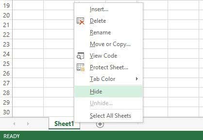
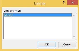
Once hidden, you can right-click on a visible sheet and select Unhide. All hidden sheets will be shown in a list and you can select the one you want to unhide.
Excel does not have the ability to hide a cell in the traditional sense that they simply disappear until you unhide them, like in the example above with sheets. It can only blank out a cell so that it appears that nothing is in the cell, but it can’t truly “hide” a cell because if a cell is hidden, what would you replace that cell with?
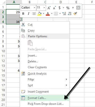
You can hide entire rows and columns in Excel, which I explain below, but you can only blank out individual cells. Right-click on a cell or multiple selected cells and then click on Format Cells.
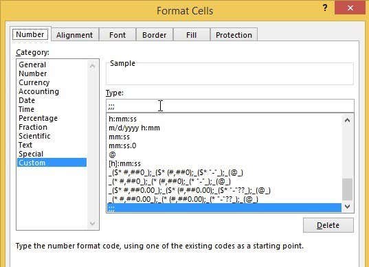
On the Number tab, choose Custom at the bottom and enter three semicolons (;;;) without the parentheses into the Type box.
Click OK and now the data in those cells is hidden. You can click on the cell and you should see the cell remains blank, but the data in the cell shows up in the formula bar.
To unhide the cells, follow the same procedure above, but this time choose the original format of the cells rather than Custom. Note that if you type anything into those cells, it will automatically be hidden after you press Enter. Also, whatever original value was in the hidden cell will be replaced when typing into the hidden cell.
Hide Gridlines
A common task in Excel is hiding gridlines to make the presentation of the data cleaner. When hiding gridlines, you can either hide all gridlines on the entire worksheet or you can hide gridlines for a certain portion of the worksheet. I will explain both options below.
To hide all gridlines, you can click on the View tab and then uncheck the Gridlines box.
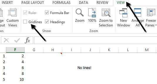
You can also click on the Page Layout tab and uncheck the View box under Gridlines.

How to Hide Rows and Columns
If you want to hide an entire row or column, right-click on the row or column header and then choose Hide. To hide a row or multiple rows, you need to right-click on the row number at the far left. To hide a column or multiple columns, you need to right-click on the column letter at the very top.
You can easily tell there are hidden rows and columns in Excel because the numbers or letters skip and there are two visible lines shown to indicate hidden columns or rows.
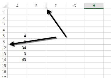
To unhide a row or column, you need to select the row/column before and the row/column after the hidden row/column. For example, if Column B is hidden, you would need to select column A and column C and then right-click and choose Unhide to unhide it.
How to Hide Formulas
Hiding formulas is slightly more complicated than hiding rows, columns, and tabs. If you want to hide a formula, you have to do TWO things: set the cells to Hidden and then protect the sheet.
So, for example, I have a sheet with some proprietary formulas that I don’t want anyone to see!

First, I will select the cells in column F, right-click and choose Format Cells. Now click on the Protection tab and check the box that says Hidden.
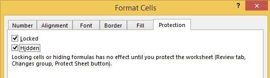
As you can see from the message, hiding formulas won’t go into effect until you actually protect the worksheet. You can do this by clicking on the Review tab and then clicking on Protect Sheet.
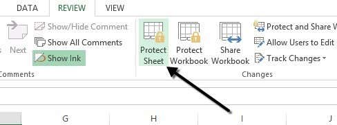
You can enter in a password if you want to prevent people from un-hiding the formulas. Now you’ll notice that if you try to view the formulas, by pressing CTRL + ~ or by clicking on Show Formulas on the Formulas tab, they will not be visible, however, the results of that formula will remain visible.
Hide Comments
By default, when you add a comment to an Excel cell, it will show you a small red arrow in the upper right corner to indicate there is a comment there. When you hover over the cell or select it, the comment will appear in a pop up window automatically.
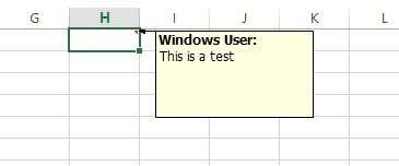
You can change this behavior so that the arrow and the comment are not shown when hovering or selecting the cell. The comment will still remain and can be viewed by simply going to the Review tab and clicking on Show All Comments. To hide the comments, click on File and then Options.
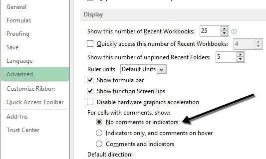
Click on Advanced and then scroll down to the Display section. There you will see an option called No comment or indicators under the For cells with comments, show: heading.
Hide Overflow Text
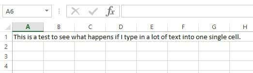
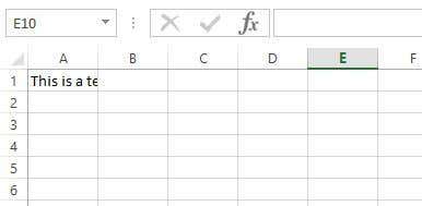
In Excel, if you type a lot of text into a cell, it will simply overflow over the adjacent cells. In the example below, the text only exists in cell A1, but it overflows to other cells so that you can see it all.
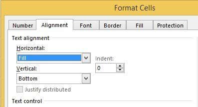
If I were to type something into cell B1, it would then cut off the overflow and show the contents of B1. If you want this behavior without having to type anything into the adjacent cell, you can right-click on the cell, choose Format Cells and then select Fill from the Horizontal Text alignment drop down box.
This will hide the overflow text for that cell even if nothing is in the adjacent cell. Note that this is kind of a hack, but it works most of the time.
You could also choose Format Cells and then check the Wrap Text box under Text control on the Alignment tab, but that will increase the height of the row. To get around that, you could simply right-click on the row number and then click on Row Height to adjust the height back to its original value. Either of these two methods will work for hiding overflow text.
Hide Workbook
I’m not sure why you would want or need to do this, but you can also click on the View tab and click on the Hide button under Split. This will hide the entire workbook in Excel! There is absolutely nothing you can do other than clicking on the Unhide button to bring back the workbook.
So now you’ve learnt how to hide workbooks, sheets, rows, columns, gridlines, comments, cells, and formulas in Excel! If you have any questions, post a comment. Enjoy!
Learn several ways to do this
Updated on September 19, 2022
What to Know
- Hide a column: Select a cell in the column to hide, then press Ctrl+0. To unhide, select an adjacent column and press Ctrl+Shift+0.
- Hide a row: Select a cell in the row you want to hide, then press Ctrl+9. To unhide, select an adjacent column and press Ctrl+Shift+9.
- You can also use the right-click context menu and the format options on the Home tab to hide or unhide individual rows and columns.
You can hide columns and rows in Excel to make a cleaner worksheet without deleting data you might need later, although there is no way to hide individual cells. In this guide, we provide instructions for three ways to hide and unhide columns in Excel 2019, 2016, 2013, 2010, 2007, and Excel for Microsoft 365.
Hide Columns in Excel Using a Keyboard Shortcut
The keyboard key combination for hiding columns is Ctrl+0.
-
Click on a cell in the column you want to hide to make it the active cell.
-
Press and hold down the Ctrl key on the keyboard.
-
Press and release the 0 key without releasing the Ctrl key. The column containing the active cell should be hidden from view.
To hide multiple columns using the keyboard shortcut, highlight at least one cell in each column to be hidden, and then repeat steps two and three above.
Hide Columns Using the Context Menu
The options available in the context — or right-click menu — change depending upon the object selected when you open the menu. If the Hide option, as shown in the image below, is not available in the context menu it is likely that you didn’t select the entire column before right-clicking.
Hide a Single Column
-
Click the column header of the column you want to hide to select the entire column.
-
Right-click on the selected column to open the context menu.
-
Choose Hide. The selected column, the column letter, and any data in the column will be hidden from view.
Hide Adjacent Columns
-
In the column header, click and drag with the mouse pointer to highlight all three columns.
-
Right-click on the selected columns.
-
Choose Hide. The selected columns and column letters will be hidden from view.
When you hide columns and rows containing data, it does not delete the data, and you can still reference it in formulas and charts. Hidden formulas containing cell references will update if the data in the referenced cells changes.
Hide Separated Columns
-
In the column header click on the first column to be hidden.
-
Press and hold down the Ctrl key on the keyboard.
-
Continue to hold down the Ctrl key and click once on each additional column to be hidden to select them.
-
Release the Ctrl key.
-
In the column header, right-click on one of the selected columns and choose Hide. The selected columns and column letters will be hidden from view.
When hiding separate columns, if the mouse pointer is not over the column header when you click the right mouse button, the hide option will not be available.
Hide and Unhide Columns in Excel Using the Name Box
This method can be used to unhide any single column. In our example, we will be using column A.
-
Type the cell reference A1 into the Name Box.
-
Press the Enter key on the keyboard to select the hidden column.
-
Click on the Home tab of the ribbon.
-
Click on the Format icon on the ribbon to open the drop-down.
-
In the Visibility section of the menu, choose Hide & Unhide > Hide Columns or Unhide Column.
Unhide Columns Using a Keyboard Shortcut
The key combination for unhiding columns is Ctrl+Shift+0.
-
Type the cell reference A1 into the Name Box.
-
Press the Enter key on the keyboard to select the hidden column.
-
Press and hold down the Ctrl and the Shift keys on the keyboard.
-
Press and release the 0 key without releasing the Ctrl and Shift keys.
To unhide one or more columns, highlight at least one cell in the columns on either side of the hidden column(s) with the mouse pointer.
-
Click and drag with the mouse to highlight columns A to G.
-
Press and hold down the Ctrl and the Shift keys on the keyboard.
-
Press and release the 0 key without releasing the Ctrl and Shift keys. The hidden column(s) will become visible.
The Ctrl+Shift+0 keyboard shortcut might not work depending on the version of Windows you’re running, for reasons not explained by Microsoft. If this shortcut doesn’t work, use another method from the article.
Unhide Columns Using the Context Menu
As with the shortcut key method above, you must select at least one column on either side of a hidden column or columns to unhide them. For example, to unhide columns D, E, and G:
-
Hover the mouse pointer over column C in the column header. Click and drag with the mouse to highlight columns C to H to unhide all columns at one time.
-
Right-click on the selected columns and choose Unhide. The hidden column(s) will become visible.
Hide Rows Using Shortcut Keys
The keyboard key combination for hiding rows is Ctrl+9:
-
Click on a cell in the row you want to hide to make it the active cell.
-
Press and hold down the Ctrl key on the keyboard.
-
Press and release the 9 key without releasing the Ctrl key. The row containing the active cell should be hidden from view.
To hide multiple rows using the keyboard shortcut, highlight at least one cell in each row you want to hide, and then repeat steps two and three above.
Hide Rows Using the Context Menu
The options available in the context menu — or right-click — change depending upon the object selected when you open it. If the Hide option, as shown in the image above, is not available in the context menu it is because you probably didn’t select the entire row.
Hide a Single Row
-
Click on the row header for the row to be hidden to select the entire row.
-
Right-click on the selected row to open the context menu.
-
Choose Hide. The selected row, the row letter, and any data in the row will be hidden from view.
Hide Adjacent Rows
-
In the row header, click and drag with the mouse pointer to highlight all three rows.
-
Right-click on the selected rows and choose Hide. The selected rows will be hidden from view.
Hide Separated Rows
-
In the row header, click on the first row to be hidden.
-
Press and hold down the Ctrl key on the keyboard.
-
Continue to hold down the Ctrl key and click once on each additional row to be hidden to select them.
-
Right-click on one of the selected rows and choose Hide. The selected rows will be hidden from view.
Hide and Unhide Rows Using the Name Box
This method can be used to unhide any single row. In our example, we will be using row 1.
-
Type the cell reference A1 into the Name Box.
-
Press the Enter key on the keyboard to select the hidden row.
-
Click on the Home tab of the ribbon.
-
Click on the Format icon on the ribbon to open the drop-down menu.
-
In the Visibility section of the menu, choose Hide & Unhide > Hide Rows or Unhide Row.
Unhide Rows Using a Keyboard Shortcut
The key combination for unhiding rows is Ctrl+Shift+9.
Unhide Rows using Shortcut Keys and Name Box
-
Type the cell reference A1 into the Name Box.
-
Press the Enter key on the keyboard to select the hidden row.
-
Press and hold down the Ctrl and the Shift keys on the keyboard.
-
Press and hold down the Ctrl and the Shift keys on the keyboard. Row 1 will become visible.
Unhide Rows Using a Keyboard Shortcut
To unhide one or more rows, highlight at least one cell in the rows on either side of the hidden row(s) with the mouse pointer. For example, you want to unhide rows 2, 4, and 6.
-
To unhide all rows, click and drag with the mouse to highlight rows 1 to 7.
-
Press and hold down the Ctrl and the Shift keys on the keyboard.
-
Press and release the number 9 key without releasing the Ctrl and Shift keys. The hidden row(s) will become visible.
Unhide Rows Using the Context Menu
As with the shortcut key method above, you must select at least one row on either side of a hidden row or rows to unhide them. For example, to unhide rows 3, 4, and 6:
-
Hover the mouse pointer over row 2 in the row header.
-
Click and drag with the mouse to highlight rows 2 to 7 to unhide all rows at one time.
-
Right-click on the selected rows and choose Unhide. The hidden row(s) will become visible.
How to Move Columns in Excel
FAQ
-
How do I hide cells in Excel?
Select the cell or cells you want to hide, then select the Home tab > Cells > Format > Format Cells. In the Format Cells menu, select the Number tab > Custom (under Category) and type ;;; (three semicolons), then select OK.
-
How do I hide gridlines in Excel?
Select the Page Layout tab, then turn off the View checkbox under Gridlines.
-
How do I hide formulas in Excel?
Select the cells with formulas you want to hide > select the Hidden checkbox on the Protection tab > OK > Review > Protect Sheet. Next, verify that Protect worksheet and contents of locked cells is turned on, then select OK.
Thanks for letting us know!
Get the Latest Tech News Delivered Every Day
Subscribe

There may be times when you want to hide information in certain cells or hide entire rows or columns in an Excel worksheet. Maybe you have some extra data you reference in other cells that does not need to be visible.
We will show you how to hide cells and rows and columns in your worksheets and then show them again.
Update, 11/3/21: Looking to hide or unhide columns in Microsoft Excel? We have an updated guide for you.
RELATED: How to Hide or Unhide Columns in Microsoft Excel
Hide Cells
You can’t hide a cell in the sense that it completely disappears until you unhide it. With what would that cell be replaced? Excel can only blank out a cell so that nothing displays in the cell. Select individual cells or multiple cells using the “Shift” and “Ctrl” keys, just like you would when selecting multiple files in Windows Explorer. Right-click on any of the selected cells and select “Format Cells” from the popup menu.

The “Format Cells” dialog box displays. Make sure the “Number” tab is active and select “Custom” in the “Category” list. In the “Type” edit box, enter three semicolons (;) without the parentheses and click “OK”.
NOTE: You might want to note what the “Type” was for each of the selected cells is before you change it so you can change the type of the cells back to what it was to show the content again.
The data in the selected cells is now hidden, but the value or the formula is still in the cell and displays in the “Formula Bar”.
To unhide the content in the cells, follow the same steps listed above, but choose the original number category and type for the cells rather than “Custom” and the three semicolons.
NOTE: If you type anything into cells in which you hid the content, it will automatically be hidden after you press “Enter”. Also, the original value in the hidden cell will be replaced with the new value or formula that you type into the cell.
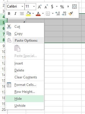
Hide Rows and Columns
If you have a large worksheet, you might want to hide some rows and columns for data you don’t currently need to view. To hide an entire row, right-click on the row number and select “Hide”.
NOTE: To hide multiple rows, select the rows first by clicking and dragging over the range of rows you want to hide, and then right-click on the selected rows and select “Hide”. You can select non-sequential rows by pressing “Ctrl” as you click on the row numbers for the rows you want to select.
The hidden row numbers are skipped in the row number column and a double line displays in place of the hidden rows.
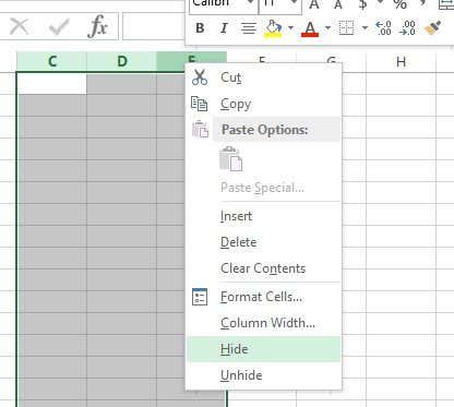
Hiding columns is a very similar process to hiding rows. Right-click on the column you want to hide, or select multiple column letters first and then right-click on the selected columns. Select “Hide” from the popup menu.
The hidden column letters are skipped in the row number column and a double line displays in place of the hidden rows.
To unhide a row or multiple rows, select the row before the hidden row(s) and the row after the hidden row(s) and right-click on the selection and select “Unhide” from the popup menu.
To unhide a column or multiple columns, select the two columns surrounding the hidden column(s), right-click on the selection, and select “Unhide” from the popup menu.
If you have a large spreadsheet and you don’t want to hide any cells, rows, or columns, you can freeze rows and columns so any headings you set up don’t scroll when you scroll through your data.
READ NEXT
- › How to Insert a Picture in Microsoft Excel
- › How to Hide or Unhide Columns in Microsoft Excel
- › How to Remove Blank Rows in Excel
- › How to Add and Remove Columns and Rows in Microsoft Excel
- › How to Copy and Paste Only Visible Cells in Microsoft Excel
- › How to Set Row Height and Column Width in Excel
- › How to Count Checkboxes in Microsoft Excel
- › How to Adjust and Change Discord Fonts
How-To Geek is where you turn when you want experts to explain technology. Since we launched in 2006, our articles have been read billions of times. Want to know more?
Making things invisible in Excel
March 20 2015 Written By: EduPristine
As kids everybody loved going to the magic show and see the things disappearing like the hats, sticks and sometimes people. Well, we can’t help you in making people disappear but we would definitely love to show you some tricks that will help you to hide certain things in Excel.
Hiding cells
Steps to hide cells in Excel
1. Select the cells that needs to be hidden. In our example it is B2:B5
2. Right click and open the format cell dailog box or you can use the shortcut key Ctrl + 1

3. On the number tab, select the custom option that is available at extreme bottom.
4. Type the formatting code as “;;;â€(3 semicolons) without the quotes and press OK.

5. The data in your cells shall be hidden(Magic).

Hiding rows and columns
Steps for hiding columns
1. Select the column from which you want to hide all the columns. In our example we shall select column G.

2. Press CTRL + Shift + Right arrow key and you will see that all the columns till XFD are selected.
3. Press Right click and select the option of hide
4. All the columns G onwards shall be hidden.

Steps for hiding rows
1. Select the row from which you want to hide all the rows. In our example, we select row 10.

2. Press CTRL + Shift + Down arrow key and you will see that all the rows till 1048576 are selected.
3. Press Right click and select the option of hide
4. All the rows from 10 onwards shall be hidden.

Hiding sheets
Steps for hiding a sheet in Excel
1. Select the sheet which you would like to hide by clicking at the tab on the bottom. In our case we are hiding sheet 2.
2. Right click and select the option of Hide.

3. You will see that your sheet is hidden

We know that these tricks won’t make you feel like a magician but they definitely will make your life a little easier. In case of any queries, mention it in the comment box and we shall get back to you at the earliest.
Watch Video – How to Unhide Columns in Excel
If you prefer written instruction instead, below is the tutorial.
Hidden rows and columns can be quite irritating at times.
Especially if someone else has hidden these and you forget to unhide it (or even worse, you don’t know how to unhide these).
While I can’t do anything about the first issue, I can show you how to unhide columns in Excel (the same techniques can also be used to unhide rows).
It may happen that one of the methods of unhiding columns/rows may not work for you. In that case, it is good to know the alternatives that can work.
There are many different situations where you may need to unhide the columns:
- Multiple columns are hidden and you want to unhide all columns at once
- You want to unhide a specific column (in between two columns)
- You want to unhide the first column
Let’s go through each for these scenarios and see how to unhide the columns.
Unhide All Columns At One Go
If you have a worksheet that has multiple hidden columns, you don’t need to go hunt each one and bring it to light.
You can do that all in one go.
And there are multiple ways to do this.
Using the Format Option
Here are the steps to unhide all columns at one go:
- Click on the small triangle at the top left of the worksheet area. This will select all the cells in the worksheet.
- Right-click anywhere in the worksheet area.
- Click on Unhide.
No matter where that pesky column is hidden, this will unhide it.
Note: You can also use the keyboard shortcut Control A A (hold the control key and hit the A key twice) to select all the cells in the worksheet.
Using VBA
If you need to do this often, you can also use VBA to get this done.
The below code will unhide column in the worksheet.
Sub UnhideColumns ()
Cells.EntireColumn.Hidden = False
EndSub
You need to place this code in the VB Editor (in a module).
If you want to learn how to do this with VBA, read a detailed guide on how to run a macro in Excel.
Note: To save time, you can save this macro in the Personal Macro Workbook and add it to the quick access toolbar. This will allow you to unhide all columns with a single click.
Using a Keyboard Shortcut
If you’re more comfortable using keyboard shortcuts, there is a way to unhide all columns with a few keystrokes.
Here are the steps:
- Select any cell in the worksheet.
- Press Control-A-A (hold the control key and press A twice). This will select all the cells in the worksheet
- Use the following shortcut – ALT H O U L (one key at a time)
If you can get hang of this keyboard shortcut, it could be a lot faster to unhide columns.
Note: The reason you need to press A twice when holding the control key is that sometimes when you press Control A, it only selects the used range in Excel (or the area that has the data) and you need to press the A again to select the entire worksheet.
Another keyword shortcut that works for some and not for others is Control 0 (from a numeric keypad) or Control Shift 0 from a non-numeric keypad. It used to work for me earlier but doesn’t work anymore. Here is some discussion on why it may happen. I suggest you use the longer (ALT HOUL) shortcut that works every time.
Unhide Columns in Between Selected Columns
There are multiple ways you can quickly unhide columns in between selected columns. The methods shown here are useful when you want to unhide a specific column(s).
Let’s go through these one-by-one (and you can choose to use that you find the best).
Using a Keyboard Shortcut
Below are the steps:
- Select the columns that contain the hidden columns in between. For example, if you are trying to unhide column C, then select column B and D.

- Use the following shortcut – ALT H O U L (one key at a time)

This will instantly unhide the columns.
Using the Mouse
One quick and easy way to unhide a column is to use the mouse.
Below are the steps:
Using the Format Option in the Ribbon
Under the home tab in the ribbon, there are options to hide and unhide columns in Excel.
Here is how to use it:
Another way of accessing this option is by selecting the columns and right clicking using the mouse. In the menu that appears, select the unhide option.

Using VBA
Below is the code that you can use to unhide columns in between the selected columns.
Sub UnhideAllColumns()
Selection.EntireColumn.Hidden = False
End Sub
You need to place this code in the VB Editor (in a module).
If you want to learn how to do this with VBA, read a detailed guide on how to run a macro in Excel.
Note: To save time, you can save this macro in the Personal Macro Workbook and add it to the quick access toolbar. This will allow you to unhide all columns with a single click.
By Changing the Column Width
There is a possibility that none of these methods work when you try to unhide column in Excel. It happens when you change the Column Width to 0. In that case, even if you unhide the column, it’s width still remains 0, and hence you can’t see it or select it.
Below are the steps to change the column width:
This is by far the most reliable way to unhide columns in Excel. If everything fails, just change the column width.
Unhide the First Column
Unhiding the first column can be a little bit tricky.
You can use many of the methods covered above, with a little bit of extra work.
Let me show you a few ways.
Use the Mouse to Drag the First Column
Even when the first column is hidden, Excel allows you to select it and drag it to make it visible.
To do this, hover the cursor on the left edge of column B (or whatever is the leftmost visible column).
The cursor would change into a double arrow pointer as shown below.

Hold the left mouse button and drag the cursor to the right. You will see that it unhides the hidden column.

Go to a Cell in the First Column and Unhide it
But how do you go to any cell in the column that’s hidden?
Good question!
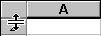
You use the Name Box (it’s left to the formula bar).

Enter A1 in the Name Box. It will instantly take you to the A1 cell. Since the first column is hidden, you won’t be able to see it, but be assured that it’s selected (you’ll still see a thin line just left of B1).
Once the hidden column cell is selected, follow the below steps:
- Click the Home tab.
- In the Cells group, click on Format.
- Hover the cursor on the ‘Hide & Unhide’ option.
- Click on ‘Unhide Columns’
Select the First Column and Unhide it
Again! How do you select it when it’s hidden?
Well, there are many different ways to skin the cat.
And this is just another method in my kitty (this is the last cat sounding reference I promise).
When you select the leftmost visible cell and drag the cursor to the left (where there are row numbers), you end up selecting all the hidden columns (even when you don’t see it).

Once you have select all the hidden columns, follow the below steps:
- Click the Home tab.
- In the Cells group, click on Format.
- Hover the cursor on the ‘Hide & Unhide’ option.
- Click on ‘Unhide Columns’
Check The Number of Hidden Columns
Excel has an ‘Inspect Document’ feature that is meant to quickly scan the workbook and give you some details about it.
And one of the things that you can do that ‘Inspect Document’ is to quickly check how many hidden columns or hidden rows are there in the workbook.
This might be useful when you get the workbook from someone and want to quickly inspect it.
Below are the steps on how to check the total number of hidden columns or hidden rows:
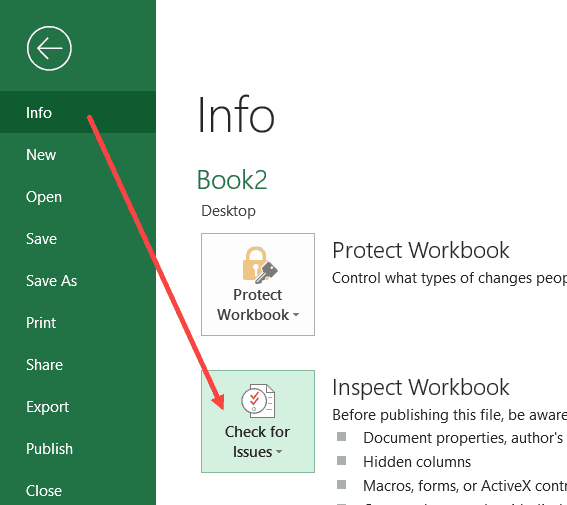
- Open the workbook
- Click on the File tab
- In the Info options, click on the ‘Check for Issues’ button (it’s next to the Inspect Workbook text).

- Click on Inspect Document.

- In the Document Inspector, make sure Hidden Rows and Columns option is checked.

- Click the Inspect button.


This will show you the total number of hidden rows and columns.

It also gives you the option to delete all these hidden rows/columns. This can be the case if there is extra data that has been hidden and is not needed. Instead of finding hidden rows and columns, you can quickly delete these from this option.
You May Also Like the following Excel Tips/Tutorials:
- How to Insert Multiple Rows in Excel – 4 Methods.
- How to Quickly Insert New Cells in Excel.
- Keyboard & Mouse Tricks that will Reinvent the Way You Excel.
- How to Hide a Worksheet in Excel.
- How to Unhide Sheets in Excel (All In One Go)
- Excel Text to Columns (7 Amazing things you can do with it)
- How to Lock Cells in Excel
- How to Lock Formulas in Excel
Last updated Monday, Dec. 5, 2022, at 10:41 a.m.
This article is based on legacy software.
At times, there may be information in your worksheet which you no longer need to see. At other times, you might be printing your worksheet and want to print only columns A–F and columns H–J, skipping column G. Rather than rearrange your worksheet for either of these examples, you can simply hide the information. You can also hide information in specific cells.
Hiding Columns
You can hide columns of your worksheet containing information that you do not need to view or do not want to print.
-
Select a cell within the column(s) to be hidden.
-
On the Home command tab, in the Cells group, click Format.
-
From the Format menu, in the Visibility section, select Hide & Unhide » Hide Columns.
The column is hidden.

Hiding Columns: Quick Menu Option
-
Right click the column ID » select Hide.
Redisplaying Columns
-
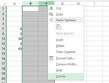
Select at least one cell from both of the columns around the hidden column(s) to be redisplayed.
EXAMPLE: If column B is hidden, select a cell from both columns A and C.
HINT: If you cannot select the appropriate cells, you can use the Go To command. -
On the Home command tab, in the Cells group, click Format.
-
From the Format menu, in the Visibility section, select Hide & Unhide » Unhide Columns.
The column reappears.

Redisplaying Columns: Quick Menu Option
This option works well for redisplaying column A, since there are not columns on both sides of column A.
-
Hold your cursor between column IDs on the right side of the hidden column.
The cursor will change to an open, double sided arrow as shown here. -
Right click » select Unhide.

Hiding Rows
You can hide rows containing information that you do not need to view or do not want to print.
-
Select a cell within the row(s) to be hidden.
-
On the Home command tab, in the Cells group, click Format.
-
From the Format menu, in the Visibility section, select Hide & Unhide » Hide Rows.
The row is hidden.

Hiding Rows: Quick Menu Option
-
Right click the row ID » select Hide.
The row is hidden.
Redisplaying Rows
-
Select at least one cell from both of the rows around the hidden row(s) to be redisplayed.
EXAMPLE: If row 5 is hidden, select a cell from rows 4 and 6.
HINT: If you cannot select the appropriate cells, you can use the Go To command. -
On the Home command tab, in the Cells group, click Format.
-
From the Format menu, in the Visibility section, select Hide & Unhide » Unhide Rows.
The row appears.

Redisplaying Rows: Quick Menu Option
This option works well for redisplaying row 1, since there are not rows on both sides of row 1.
-
Hold your cursor between row IDs where the hidden row is located.
The cursor will change to an open, double sided arrow as shown here. -
Right click » select Unhide.
Hiding Cell Contents
You have the ability to hide the contents of individual cells if you do not need to view their contents or you simply do not want to print certain cells.
-
Select the cell(s) to be hidden.
-
From the Home command tab, in the Cells group, click Format
» select Format Cells…
The Format Cells dialog box appears. -
Select the Number tab.
-
Under Category, select Custom.
-
In the Type text box, type three semicolons ( ;;; ).
-
Click OK.
The cells are now hidden.
 » select Format Cells…
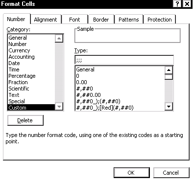
To redisplay cell information:
-
Select the cell(s) to be redisplayed.
-
From the Home command tab, in the Cells group, click Format
» select Format Cells…
The Format Cells dialog box appears. -
Select the Number tab.
-
Under Category, make the appropriate selection.
The dialog box refreshes to display options corresponding to the selected category. -
Select the desired options.
-
Click OK.
The cell(s) reappear.
 » select Format Cells…
Was this article helpful?
Yes
No
View / Print PDF