Cell styles for excel

To apply several formats in one step, and to make sure that cells have consistent formatting, you can use a cell style. A cell style is a defined set of formatting characteristics, such as fonts and font sizes, number formats, cell borders, and cell shading. To prevent anyone from making changes to specific cells, you can also use a cell style that locks cells.

Microsoft Office Excel has several built-in cell styles that you can apply or modify. You can also modify or duplicate a cell style to create your own, custom cell style.

Important: Cell styles are based on the document theme that is applied to the whole workbook. When you switch to another document theme, the cell styles are updated to match the new document theme.

1. Select the cells that you want to format. For more information, see Select cells, ranges, rows, or columns on a worksheet.

2. On the Home tab, in the Styles group, click the More dropdown arrow in the style gallery, and select the cell style that you want to apply.

   

1. On the Home tab, in the Styles group, click the More dropdown arrow in the style gallery, and at the bottom of the gallery, click New Cell Style.

2. In the Style name box, type an appropriate name for the new cell style.

3. Click Format.

4. On the various tabs in the Format Cells dialog box, select the formatting that you want, and then click OK.

5. Back in the Style dialog box, under Style Includes (By Example), clear the check boxes for any formatting that you do not want to include in the cell style.

6. Click OK.

1. On the Home tab, in the Styles group, click the More dropdown arrow in the style gallery.

   

2. Do one of the following:

   • To modify an existing cell style, right-click that cell style, and then click Modify.

   • To create a duplicate of an existing cell style, right-click that cell style, and then click Duplicate.

3. In the Style name box, type an appropriate name for the new cell style.

   Note: A duplicate cell style and a renamed cell style are added to the list of custom cell styles. If you do not rename a built-in cell style, the built-in cell style will be updated with any changes that you make.

4. To modify the cell style, click Format.

5. On the various tabs in the Format Cells dialog box, select the formatting that you want, and then click OK.

6. In the Style dialog box, under Style Includes, select or clear the check boxes for any formatting that you do or do not want to include in the cell style.

You can remove a cell style from data in selected cells without deleting the cell style.

1. Select the cells that are formatted with the cell style that you want to remove. For more information, see Select cells, ranges, rows, or columns on a worksheet.

2. On the Home tab, in the Styles group, click the More dropdown arrow in the style gallery.

   

3. Under Good, Bad, and Neutral, click Normal.

You can delete a predefined or custom cell style to remove it from the list of available cell styles. When you delete a cell style, it is also removed from all cells that are formatted with it.

1. On the Home tab, in the Styles group, click the More dropdown arrow in the style gallery.

   

2. To delete a predefined or custom cell style and remove it from all cells that are formatted with it, right-click the cell style, and then click Delete.

   Note: You cannot delete the Normal cell style.

1. Select the cells that you want to format. For more information, see Select cells, ranges, rows, or columns on a worksheet.

2. On the Home tab, in the Styles group, click Cell Styles.

   

   Tip: If you do not see the Cell Styles button, click Styles, and then click the More button next to the cell styles box.

3. Click the cell style that you want to apply.

1. On the Home tab, in the Styles group, click Cell Styles.

   

   Tip: If you do not see the Cell Styles button, click Styles, and then click the More button next to the cell styles box.

2. Click New Cell Style.

3. In the Style name box, type an appropriate name for the new cell style.

4. Click Format.

5. On the various tabs in the Format Cells dialog box, select the formatting that you want, and then click OK.

6. In the Style dialog box, under Style Includes (By Example), clear the check boxes for any formatting that you do not want to include in the cell style.

1. On the Home tab, in the Styles group, click Cell Styles.

   

   Tip: If you do not see the Cell Styles button, click Styles, and then click the More button next to the cell styles box.

2. Do one of the following:

   • To modify an existing cell style, right-click that cell style, and then click Modify.

   • To create a duplicate of an existing cell style, right-click that cell style, and then click Duplicate.

3. In the Style name box, type an appropriate name for the new cell style.

   Note: A duplicate cell style and a renamed cell style are added to the list of custom cell styles. If you do not rename a built-in cell style, the built-in cell style will be updated with any changes that you make.

4. To modify the cell style, click Format.

5. On the various tabs in the Format Cells dialog box, select the formatting that you want, and then click OK.

6. In the Style dialog box, under Style Includes, select or clear the check boxes for any formatting that you do or do not want to include in the cell style.

You can remove a cell style from data in selected cells without deleting the cell style.

1. Select the cells that are formatted with the cell style that you want to remove. For more information, see Select cells, ranges, rows, or columns on a worksheet.

2. On the Home tab, in the Styles group, click Cell Styles.

   

   Tip: If you do not see the Cell Styles button, click Styles, and then click the More button next to the cell styles box.

3. Under Good, Bad, and Neutral, click Normal.

You can delete a predefined or custom cell style to remove it from the list of available cell styles. When you delete a cell style, it is also removed from all cells that are formatted with it.

1. On the Home tab, in the Styles group, click Cell Styles.

   

   Tip: If you do not see the Cell Styles button, click Styles, and then click the More button next to the cell styles box.

2. To delete a predefined or custom cell style and remove it from all cells that are formatted with it, right-click the cell style, and then click Delete.

   Note: You cannot delete the Normal cell style.

Need more help?

You can always ask an expert in the Excel Tech Community or get support in the Answers community.

Quickly format a cell by choosing a cell style. You can also create your own cell style in Excel. Quickly format a range of cells by choosing a table style.

1. For example, select cell B2 below.

2. On the Home tab, in the Styles group, choose a cell style.

Result.

To create your own cell style, execute the following steps.

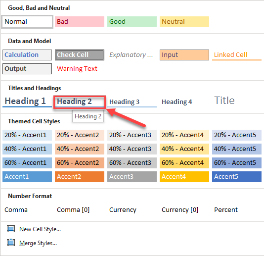
3. On the Home tab, in the Styles group, click the bottom right down arrow.

Here you can find many more cell styles.

4. Click New Cell Style.

5. Enter a name and click the Format button to define the Number Format, Alignment, Font, Border, Fill and Protection of your cell style. Simply uncheck a check box if you don’t want to control this type of formatting.

6. Click OK.

7. On the Home tab, in the Styles group, apply your own cell style.

Result.

Note: right click a cell style to modify or delete it. Modifying a cell style affects all cells in a workbook that use that cell style. This can save a lot of time. A cell style is stored in the workbook where you create it. Open a new workbook and click on Merge Styles (under New Cell Style) to import a cell style (leave the old workbook with the cell style open).

Home > Microsoft Excel > How to Use Cell Styles in Excel: A Step-by-Step Guide

(Note: This guide on how to use cell styles in Excel is suitable for all Excel versions including Office 365)

Consider an Excel sheet that has data of different types and formats. The data might be downloaded, inserted, or circulated between users one after the other. In those cases, each data might have different formatting depending on the user settings. This will make the data unpleasant to look at and hinders its readability.

You would then want to modify and organize the data in a well-formatted and orderly fashion. You can select each cell or cell range and modify the look and format of the cell manually. However, this task can be a little daunting and time-consuming. 

Here, using the Cell Styles option in Excel you can easily modify the formatting and profile of the cell and its contents with the click of a button.

In this article, I will show you how to apply built-in styles, create custom styles, and remove the cell styles in Excel when not necessary.

You’ll Learn:

• What Are Cell Styles in Excel?
• How to Use Cell Styles in Excel?
  • Apply Built-In Cells Styles
  • Create a Custom Cell Style
  • Customize an Existing Style
  • Duplicate a Cell Style
  • Remove the Cell Style
  • Delete Cell Styles

Watch this video on How to Use Cell Styles in Excel in an easy way

Related Reads:

The 7 Golden Rules of Excel Spreadsheet Design

How to Create Excel Drop Down List With Color?

How to Graph a Function in Excel? 2 Easy Ways

What Are Cell Styles in Excel?

Cell Style refers to formatting and features that you can customize in a cell. The features that can be modified using cell styles include the font style, font color, color fill, format type, cell borders, cell color, and much more. 

Cell Styles have similar characteristics to Conditional Formatting. In Conditional Formatting, the format of the cells is changed when specific conditions or criteria are met. Whereas, Cell Styles are static i.e. you can change the cell styles whenever you want based on your needs.

The cell styles option will be very useful when you have to change the style formatting of a group of cells altogether instead of changing them one by one. You can create a particular cell style by including all the cell format aspects like font color, size, font style, fill, borders, etc., and then use them whenever needed. 

Using the built-in or custom-created cell styles will make all the cells look more consistent and give a professional finish to the data, thereby making it easier to read.

There are a variety of options available when it comes to cell styling in Excel. You can do the following: 

• Apply the Built-In Cell Styles in Excel
• Create a Custom Cell Style
• Copy and Duplicate an Existing Cell Style
• Modify an Existing Cell Style
• Remove the Cell Style from the Cells
• Delete a Cell Style

In this guide, I will explain how to use Cell Styles with an example. 

Consider an example, where you have a consolidated list of sales made by an automobile company in 11 years. 

When you enter the data onto an Excel sheet, the formatting will be different for numbers and texts. Also, there is no distinction or highlights to show the differentiation of data. You can now use the Cell Styles to format the cells and their contents.

How to Use Cell Styles in Excel?

We have recently understood what cell styles are and how you can customize cells using them. Let us now see how to use cell styles effectively to get the best profile overall. 

Apply Built-In Cells Styles

First, let us see how to apply the built-in cell styles in Excel. This is the first and foremost step when it comes to formatting a cell. After this, we can see how to create custom styles and change them.

• First, select a cell or a group of cells. In this case, let us apply the cell style to the headers i.e. the vehicle types from rows A5 to F5.

• Now, navigate to Home. Under the Styles section, click on the dropdown from Cell Styles. When you click the dropdown, you can see a variety of cell styles with different fill colors, border colors, and fonts. Since we are formatting the heading, let us select the Heading 2 style.

• Once you select your desired cell style, the style with the formatting will be applied to the selected cells.

Create a Custom Cell Style

Even though there are a variety of cell styles to choose from, there might be some instances where you might not be satisfied with the available options. In such instances, you can create your custom style with the necessary options to suit your purpose.

• To create a custom cell style, first, select a cell or range of cells. 

• Go-to Home. From the dropdown from Cell Styles, click on New Cell Style.

• This opens up a Style dialog box. Under Styles Includes (By example), you can see the different format options the cell is formatted for. You can choose to uncheck the checkboxes if you don’t want to include that particular aspect in the cells. 

Now, let’s get to formatting the styles. 

• From the Style Name textbox, you can set the name of the custom style.

• To change the other aspects of the cell, click on Format. This opens up the Format dialog box. Under the tabs provided, you can change the formatting type, font, border, color, and alignment of the cells. Additionally, you can also choose to lock and protect the cells to prevent them from being edited.

• After making all the necessary changes, click OK.

• This adds the custom style in the Cell Styles dropdown. 

• If you want to change the cell style, you can do it with a click. Select the cells you want to format, then select the custom format you created from the Cell Styles dropdown. 

Suggested Reads:

How to Create an Excel Slicer? 2 Easy Ways

How to Convert Excel to Word? 2 Easy Methods

How to Make a Pareto Chart Excel Dashboard? 4 Easy Steps

Customize an Existing Style

When working on cell styles, you might sometimes feel the existing styles to be a little inadequate. You also don’t want to create a cell style from scratch. In such cases, you can just tweak and modify the existing styles a little to create your style. 

• To modify an existing style, click on the dropdown from Cell Styles.

• Right-click on the style you want to customize and click on Modify. 

• When you click on Modify, the Style dialog box opens. 

• In the same way, check the checkboxes for the formatting features you want to include in the cell style. For additional settings related to font style, color, border, alignment, and protection, click on Format. 

• This opens the Format Cells dialog box. Select and customize all the necessary options and click on OK.

• Now, if you click on the dropdown from Cell Styles, you can see the default built-in font modified based on your input options.

Note: To change the modified built-in style to its default state, right-click on the style and click on Delete.

Duplicate a Cell Style

It is always a good practice to copy a cell style and then modify them instead of overriding the existing cell style. In such cases, you can duplicate a built-in or custom cell style and modify them.

• To duplicate a cell style, go to Home and click on the dropdown from Cell Styles. This shows you a list of built-in and custom cell styles.

• Now, right-click on the style you want to duplicate and select Duplicate.

• This in turn opens the Styles dialog box. Select the format features you want to include using the Format option. 

• Click OK.

• Now, the duplicated font gets saved under the Custom section of the Cell Styles dropdown. You can now use the style whenever needed. 

Remove the Cell Style

In case you are not satisfied with the cell style, you can either change the cell style or remove them. 

• To remove the cell style, first, select the cells with a particular cell style. 

• Navigate to Home. Click on the dropdown from Cell Styles. Select Normal.

• This removes the cell styles for the formatted cells and the cells are reset to the default cell styling.

Delete Cell Styles

Often, deleting and removing a particular thing might be synonymous. Here, deleting a cell style and removing a cell style are two different things. When removing, you remove the formatting of the cells and change them back to their default state. When you delete a Cell Style, you delete the particular cell style from the repository. 

You can delete a cell style if you are not satisfied with the style formatting or if you won’t need them anymore. 

• To delete a cell style, go to Home. Click on the dropdown from the Cell Styles. 

• Right-click on the cell style you want to delete and click on Delete.

• This deletes the particular cell style from the cell style repository.

Note: When you delete a cell style, all the cells which have the particular cell style will be deleted and the cells will be set to Normal (default) cell style.

Also Read:

How to Create a Funnel Chart in Excel? 2 Useful Ways

How to Insert a Hyperlink in Excel? 3 Easy Ways

How to Save Excel Chart as Image? 4 Simple Ways

Frequently Asked  Questions

Closing Thoughts

Cell Styles help combine a lot of attributes and aspects of a cell into a single click. They are an essential factor in Excel that greatly help in improving the readability and presentability of the data. 

In this article, we saw how to apply a cell style, modify, duplicate a cell style, create a custom cell style, remove a cell style, and even delete them. Depending on your needs, you can choose to use any option that suits your purpose the best. 

Please visit our free resources center for more high-quality Excel guides. 

Ready to take the next step and hone your skills in Excel?

Simon Sez IT has been teaching Excel for over ten years. For a low, monthly fee you can get access to 140+ IT training courses. Click here for advanced Excel courses with in-depth training modules.

How to Format Excel Spreadsheets Using Cell Styles

Create professional-looking work

Updated on February 23, 2020

Formatting your Excel spreadsheets gives them a more polished look, and can also make it easier to read and interpret the data, and thus better suited for meetings and presentations. Excel has a collection of pre-set formatting styles to add color to your worksheet that can take it to the next level.

These instructions apply to Excel for Microsoft 365 and Excel 2019, 2016, 2013, and 2010.

What Is a Cell Style?

A cell style in Excel is a combination of formatting options, including font sizes and color, number formats, cell borders, and shading that you can name and save as part of the worksheet.

Apply a Cell Style

Excel has many built-in cell styles that you can apply as is to a worksheet or modify as desired. These built-in styles can also serve as the basis for custom cell styles you can save and share between workbooks.

1. Select the range of cells you want to format.

2. On the Home tab of the ribbon, select the Cell Styles button in the Styles section, to open the gallery of available styles.

3. Select the desired cell style to apply it.

Customize Cell Styles

One advantage of using styles is that if you modify any cell style after applying it in a worksheet, all cells using that style automatically update to reflect the changes.

Further, you can incorporate Excel’s lock cells feature into cell styles to prevent unauthorized changes to specific cells, worksheets, or workbooks.

You can also customize cell styles either from scratch or using a built-in style as a starting point.

1. Select a worksheet cell.

2. Apply all desired formatting options to this cell.

3. On the Home tab of the ribbon, select the Cell Styles button in the Styles section, to open the gallery of available styles.

4. Select New cell styles at the bottom of the gallery.

5. Type a name for the new style in the Style name box.

6. Select the Format button in the Style dialog box to open the Format Cells dialog box.

7. Select a tab in the dialog box to view the available options.

8. Apply all desired changes.

9. Select OK to return to the Style dialog box.

10. Underneath the name is a list of the formatting options that you selected. Clear the checkboxes for any unwanted formatting.

11. Select OK to close the dialog box and return to the worksheet.

The new style’s name will now appear at the top of the Cell Styles Gallery under the Custom heading. To apply your style to cells in a worksheet, follow the steps above for using a built-in style.

To edit cell formatting, launch the Cell Styles Gallery and right-click on a cell style and choose Modify > Format. The right-click menu also includes a Duplicate option.

Copy a Cell Style to Another Workbook

When you create a custom cell style in a workbook, it’s not available across Excel. You can easily copy custom styles to other workbooks, though.

1. Open the first workbook containing the custom style you want to copy.

2. Open the second workbook.

3. In the second workbook, select Cell Styles on the ribbon to open the Cell Styles gallery.

4. Select Merge Styles at the bottom of the gallery to open the Merge Styles dialog box.

5. Select the name of the first workbook and choose OK to close the dialog box.

An alert box will pop up asking if you want to merge styles with the same name. Unless you have custom styles with the same name but different formatting options in both workbooks, click the Yes button to complete the transfer into the destination workbook.

Remove Cell Style Formatting

Finally, you can remove any formatting you apply to a cell without deleting the data or the saved cell style. You can also delete a cell style if you no longer want to use it.

1. Select the cells that are using the cell style that you want to remove.

2. On the Home tab of the ribbon, select the Cell Styles button in the Styles section, to open the gallery of available styles.

3. In the Good, Bad, and Neutral section near the top of the gallery, select Normal to remove all applied formatting.

The above steps can also be used to remove formatting that has been applied manually to worksheet cells.

Delete a Style

You can delete any built-in and custom cell styles from the Cell Styles gallery except for Normal, which is the default. When you delete a style, any cell that was using it will lose all associated formatting.

1. On the Home tab of the ribbon, select the Cell Styles button in the Styles section, to open the gallery of available styles.

2. Right-click on a cell style to open the context menu and choose Delete. The cell style is immediately removed from the gallery.

Thanks for letting us know!

Get the Latest Tech News Delivered Every Day

Subscribe

Стили в Excel – это инструмент, который позволяет существенно упростить и ускорить процесс форматирования документа. Стилям форматирования можно дать определение как сохраненные под определенным названием готовых настроек форматов. Их можно легко присвоить одной или множеству ячеек.

Присвоение стилей форматирования ячейкам

В каждом стиле определены следующие настройки:

1. Шрифт (тип, размер, цвет и т.п.).
2. Формат отображения чисел.
3. Границы ячеек.
4. Заливка и узоры.
5. Защита ячеек.

Благодаря стилям все листы легко и быстро отформатировать. А если мы вносим изменение в стиль, то эти изменения автоматически присваиваются всем листам, которые им отформатированы.

В Excel предусмотрена библиотека из готовых тематических стилей, а так же присутствует возможность создавать собственные пользовательские стили.

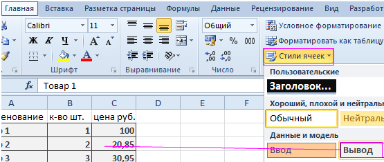
Чтобы воспользоваться библиотекой встроенных стилей необходимо:

1. Виделите в указанной на рисунке таблице не отформатированную область ячеек, но без заголовка.



2. Выберите инструмент: «Главная»-«Стили»-«Стили ячейки»



3. Из выпадающего списка миниатюр предварительного просмотра стиля, выберите понравившейся Вам.



Создание пользовательского стиля по образцу

Теперь создадим свой пользовательский стиль, но по образцу уже готового:

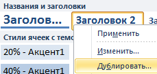
1. Выделите первую строку таблицы, чтобы отформатировать ее заголовок.
2. Отобразите выпадающий список встроенных стилей и щелкните правой кнопкой мышки по «Заголовок 2». А из контекстного меню выберите опцию «Дублировать».



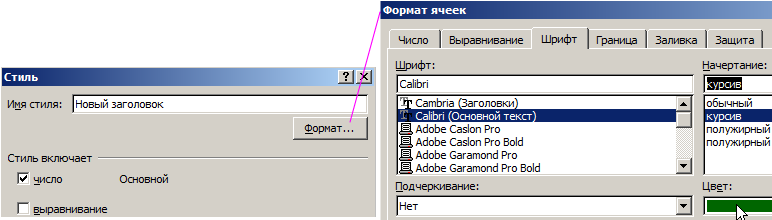
3. В диалоговом окне, укажите имя стиля «Новый заголовок» и, не изменяя настроек жмите на кнопку «Формат».



4. В появившемся окне «Формат ячеек» внесите свои изменения. На вкладке шрифт укажите темно-зеленый цвет. А шрифт измените на «курсив». Далее ОК и снова ОК.
5. Присвойте Ваш стиль на главной панели: «Стили ячейки»-«Пользовательские»-«Новый заголовок».

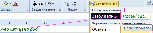
Таким образом, на основе встроенного стиля мы создали дубликат, который изменили под свои потребности.

Можно ли изменять стиль в Excel? В принципе можно было и не создавать дубликат, а в контекстном меню сразу выбрать «Изменить». Все изменения любого встроенного стиля по умолчанию, сохранились бы только в текущей книге. На настройки программы они не влияют. И при создании новой книги библиотека стилей отображается стандартно без изменений.

Можно ли удалить стиль в Excel? Конечно можно, но только в рамках одной книги. Например, как удалить пользовательские стили в Excel?

Выбираем желаемый стиль на главной панели: «Стили ячейки» и в разделе «Пользовательские» щелкаем правой кнопкой мышки. Из появившегося контекстного меню выберем опцию «Удалить». В результате ячейки очистятся от форматов заданных соответствующим стилем.

Точно так же можно удалить стили в Excel встроенные по умолчанию в библиотеке, но данное изменение будет распространяться только на текущую книгу.

Создать стиль по формату ячейки

Но что если нужно создать стиль на основе пользовательского формата ячеек, который задан обычным способом.

1. Задайте пустой ячейке формат с изменением заливки и цвета шрифта.
2. Теперь выделите эту исходную ячейку и выберите инструмент на главной панели: «Стили ячейки»-«Создать стиль ячейки».
3. В окне «Стиль» укажите имя стиля «Как в ячейке1» и нажмите ОК.

Теперь у Вас в разделе стилей «Пользовательские» отображается имя «Как в ячейке1». Принцип понятен.

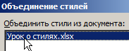
Все выше описанные стилевые форматы сохраняются в рамках файла текущей книги Excel. Поэтому для дальнейших действий сохраните эту книгу под названием «Урок о стилях.xlsx».

Копирование стиля в другие книги

Иногда возникает необходимость использовать текущие стили и в других книгах. Для этого можно просто скопировать их:

1. Создайте новую книгу, в которой будем использовать пользовательский стиль «Как в ячейке1».
2. Откройте книгу «Урок о стилях.xlsx» из сохраненным исходным требуемым нам стилем.
3. Выберите инструмент на главной закладке: «Стили ячейки»-«Объединить». И в окне «Объединение стилей» укажите на нужную нам книгу и ОК.

Теперь все пользовательские или измененные форматы из исходной книги скопированы в текущую.

Если Вам нужно будет часто использовать один стиль в разных книгах, тогда есть смысл создать специальную книгу со своими стилями и сохранить ее как шаблон. Это будет значительно удобнее чем каждый раз копировать… А все преимущества шаблонов подробнее рассмотрим на следующих уроках.

Форматирование в Excel – это очень утомительное, но важное задание. Благодаря стилям мы можем существенно ускорить и упростить данный рабочий процесс. Сохраняя при этом точную копию форматов ячеек в разных листах и книгах.

See all How-To Articles

In this article, you will learn how to apply different cell styles in Excel.

Apply Cell Styles

Excel allows us to format cells with predefined cell styles. These include different font sizes and styles, backgrounds, border styles, colors, etc. We’ll use the following data range with sales data to explain applying cell styles.

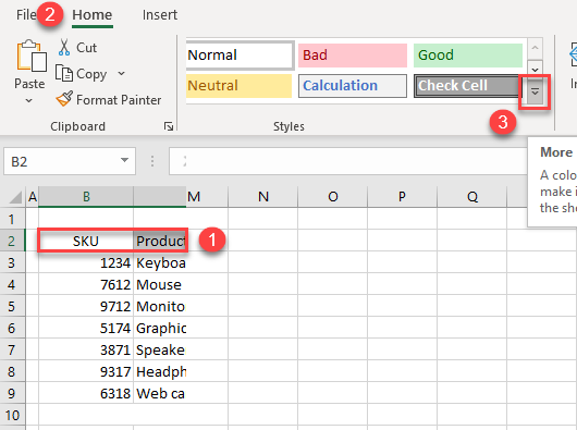
Let’s first format the table headings (range B2:F2). To do this, (1) select the range, then in the Ribbon, (2) go to the Home tab and in the Styles part, (3) click on More.

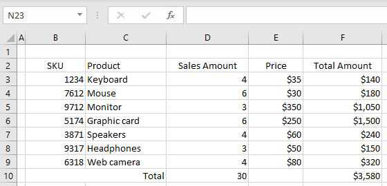
In the offered menu, we can choose a cell style. In this case, we will use a style for headings and titles (Heading 2). As a result, the range of cells B2:F2 is formatted as shown in the picture below.

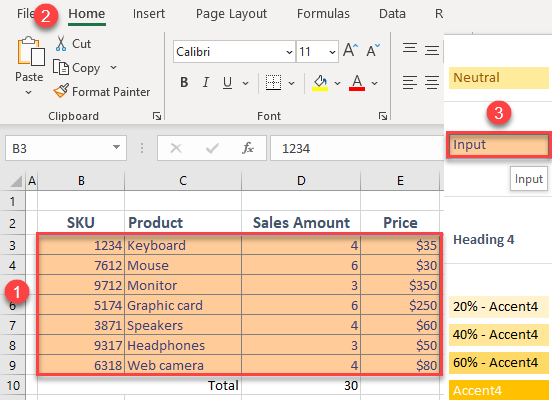
Next, we can format range B3:E9 as input cells. In order to achieve this, (1) select the range. Then in the Ribbon, (2) go to the Home tab and in the Styles part, (3) click on More. In the offered menu, we’ll choose a cell style. In this case, we will use a style for input data: (4) Input. As a result, the range of cells B3:E9 is formatted as shown in the picture below.

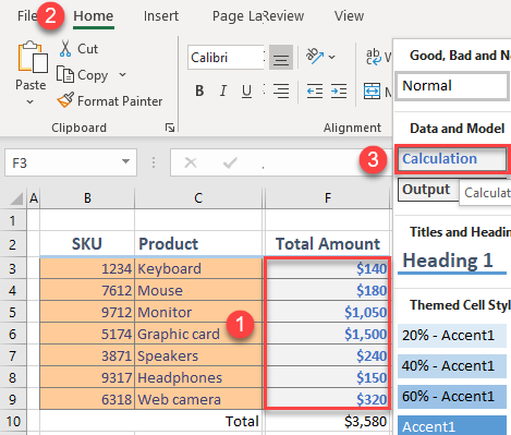
In the same way, we can format cells F3:F9 as calculation cells. Let’s (1) select the range, then in the Ribbon, (2) go to the Home tab and in the Styles part, (3) click on More. In the offered menu, we’ll choose a cell style. In this case, we will use a style for calculation data: (4) Calculation. As a result, the range of cells F3:F9 is formatted as shown in the picture below.

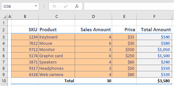
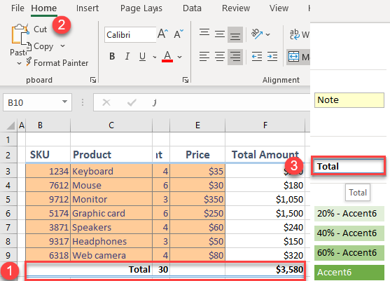
Finally, we’ll format cells B10:F10 as Total cells. (1) Select the range, then in the Ribbon, (2) go to the Home tab and in the Styles part, (3) click on More. In the offered menu, we’ll choose a cell style. In this case, we will use a style for totals and headings: (4) Total. As a result, the range of cells B10:F10 is formatted as shown in the picture below.

Modify Cell Styles

We can also modify any style that Excel offers by default. Let’s use the previous example and change the font color of the Total Amounts column (cells F3:F10) to blue. In order to achieve this, we need first to (1) select the range, then in the Ribbon, (2) go to the Home tab in the Styles part (3) right-click the current cell style (Calculation) and (4) click on Modify.

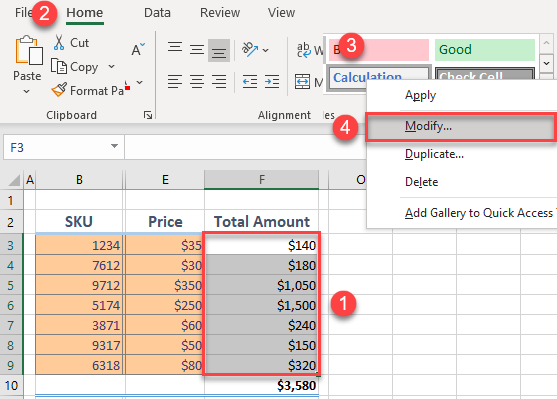
In the pop-up screen, (1) go to Format. Then in the new screen, (2) go to the Font tab, (3) click on the Color drop down and (4) choose Blue.

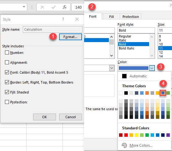
As a result, we get the style shown below, with Calculation fields having blue font.

In the same way as in the previous step, we could change number format, set bold or italic, change font size, etc.

Что такое стиль

Стиль в Microsoft Excel — это сохраненная совокупность параметров форматирования ячейки. Единожды создав стиль, его затем можно многократно применять к другим ячейкам, моментально оформляя их нужным вам образом, что неимоверно ускоряет повседневную работу в Excel.

Весь список стилей доступен на вкладке Главная в группе Стили (Home — Styles):

Важно отметить, что стиль — это не только внешнее оформление (цвет, шрифт, заливка), как многие думают. В стиле ячейки Excel можно сохранить:

• Числовой формат (денежный, процентый, даты/времени…), в том числе и пользовательский (кг, шт, °С…)
• Параметры выравнивания (по горизонтали и вертикали), направление текста, перенос по словам.
• Параметры шрифта (цвет, начертание, размер…)
• Цвет и тип заливки (сплошная, градиент)
• Обрамление ячейки (тип, толщина и цвет линий с каждой стороны и внутри)
• Параметры защиты (нужно ли защищать ячейку и прятать в ней формулы при включении защиты листа)

Как создать стиль

Выделите ячейку, оформление которой хотите сохранить в стиле (или пустую ячейку, если хотите создать стиль «с нуля») и на вкладке Главная в группе Стили выберите команду Создать стиль ячейки (New cell style).

В открывшемся окне можно отметить флажками, какие именно параметры ячейки должны сохраняться в новом стиле и, нажав кнопку Формат (Format), настроить их более детально.

Чтобы создать стиль на основе уже имеющегося стиля, можно просто щёлкнуть правой кнопкой мыши по нужному стилю и выбрать команду Дублировать (Duplicate):

Там же в контекстном меню любой стиль можно удалить или изменить его параметры.

Всё весьма несложно и даже слегка скучновато, не правда ли? Так что давайте перейдем к практическим примерам.

Стиль для целых чисел с разделителями

Начнем простого для затравки.

На Главной вкладке в группе Число есть кнопки для быстрого применения основных числовых форматов, которые вам, я уверен, хорошо знакомы:

Лично меня всегда безмерно удивляло, почему в этом наборе нет самого нужного — формата, где отображается только целая часть числа с пробелом через три разряда? Денежный — есть, процентный — есть, а вот удобного формата для обычных чисел — почему-то нет.

Кстати, третья иконка со значком «000», про которую обычно думают в этом случае, делает совершенно не то, что нужно — она не убирает дробную часть, да ещё и зачем-то выводит вместо нуля прочерк, как в финансовом формате. Совсем не оно.

Давайте устраним этот недостаток, создав свой стиль. Выбираем, как было описано выше, последовательно Главная — Стили — Создать стиль ячейки (Home — Styles — New cell style). В окне создания стиля введём его имя и снимем все галочки, кроме первой, чтобы создаваемый нами стиль не влиял ни на какие другие параметры ячейки, кроме числового формата. Затем жмём кнопку Формат (Format) и в знакомом окне выбираем Числовой (Number) без десятичных знаков и с разделителем групп разрядов:

Жмём на все ОК и теперь у нас есть стиль для наглядного форматирования чисел — красота!

Стили для своих единиц измерения (шт, чел, упак, кг…)

Исходно в Excel в качестве единиц измерения есть только валюты и проценты. Если же по работе вы сталкиваетесь с необходимостью использовать другие единицы измерения (шт, чел, л, т, кг, упак и т.д.), то имеет смысл создать для этого специальный стиль.

Выполняем те же действия, что и в предыдущем пункте, но в окне Формат ячеек выбираем на вкладке Число опцию (все форматы). В поле Тип (Type) вводим маску (шаблон) для нашего пользовательского формата:

# ##0″ шт»

Такой шаблон говорит Excel, что мы хотим выводить только целую часть числа и добавить к ней пробел и ШТ. Обратите внимание, что первый пробел здесь нужен для разделения тысяч-миллионов-миллиардов, а второй — чтобы число и текст не слиплись. И вот этот второй должен обязательно находиться внутри кавычек вместе с ШТ.

После применения такого стиля получим красивое представление для штук:

Аналогичным образом можно сделать и дробный формат, например, для килограмм. В этом случае для отображения трёх знаков после запятой (для граммов) потребуется лишь добавить к нашему шаблону нули:

# ##0,000″ шт»

Стили для тысяч (К) и миллионов (М)

Ещё один пример весьма распространённой задачи — компактное представление для очень больших чисел. Вы наверняка видели варианты для тысяч с буквой «К» (1289 = 1,3К), для миллионов с буквой «М» (1 595 000 = 1,6М) или что-то похожее. Чтобы создать такие стили нам опять потребуется пользовательский формат, но с немного другим шаблоном:

Обратите внимание на пробел (без кавычек) после нуля — именно он, являясь разделителем разрядов, округляет наше исходное значение до тысяч. Если поставите два пробела — получите округление до миллионов, три — до миллиардов и т.д.

Если нужно показать после запятой один или несколько знаков (например 3,5K или 5,23М), то добавляем нули, как в прошлом примере:

# ##0,0 «K»

# ##0,00  «M»

Вместо международных «К» и «М» можно, само-собой, использовать и наши привычные » тыс.руб» и » млн.$» — кому как привычнее.

Стиль с цветом и процентами для отклонения от плана

Предположим, что у нас есть таблица со значениями плана и факта и вычисленным столбцом отклонения в процентах по классической формуле:

Давайте создадим для последнего столбца особый стиль, который будет:

• Положительные значения выводить зелёным цветом шрифта, со знаком плюс перед значенем процентов.
• Отрицательные значения — красным цветом и с минусом, соответственно.

Создаём стиль как и ранее, а вот маска формата будет хитрая:

[Цвет10]+0%;[Красный]-0%;0%

Давайте разберём её подробнее:

• Маска формата здесь состоит из 3 фрагментов, разделенных точкой с запятой. Первая применяется, если число в ячейке больше нуля, вторая — если меньше нуля, третья — если число равно нулю.
• Отклонения от плана мы хотим указывать явно — с плюсом (перевыполнение) и минусом (невыполнение), поэтому знаки плюса и минуса явно прописываем в шаблоне.
• Перед маской в каждом блоке можно указать в квадратных скобках цвет шрифта — словом (красный, синий, зеленый, желтый, черный, белый) или с помощью кода (Цвет1, Цвет2 и т.д.) Всего поддерживается 56 цветов — выбирайте любой на ваш вкус:

  

После применения созданного стиля картинка станет существенно приятнее:

Стили со значками и спецсимволами

Чтобы сделать ещё красивее, можно вместо плюса и минуса выводить символы стрелки вверх и вниз, соответственно. Для этого выделим любую пустую ячейку на листе и вставим туда наши значки, через команду Вставка — Символ (Insert — Symbol):

Затем выделим вставленные символы в ячейке или в строке формул и скопируем их с помощью сочетания Ctrl+C.

Теперь, при создании стиля для отличий из предыдущего пункта, останется вставить с помощью Ctrl+V эти символы в нашу маску формата вместо плюса и минуса:

[Цвет10]↑0%;[Красный]↓0%;0%

После применения такого стиля наше отклонение от плана станет ещё нагляднее:

Думаю, понятно, что такой трюк со вставкой спецсимволов позволит аналогичным образом создать стили для отображения любых нестандартных единиц измерения:

Стили со сложными условиями и эмодзи

Предположим, что у нас есть таблица с результатами экзаменов студентов или аттестации сотрудников:

Задача — показать рядом с каждым результатом его графическое представление в виде иконки (эмодзи) по следующей логике:

• больше или равно 80 баллов — отлично
• от 40 до 80 — хорошо
• меньше 40 — плохо

Создаем новый стиль, где в шаблоне числового формата задаём:

Здесь маска тоже состоит из трёх фрагментов и каждый фрагмент применяется только при выполнении условия, заданного в квадратных скобках перед ним. Если первые два условия для ячейки не выполняются, то форматирование происходит по последнему, третьему шаблону.

Эмодзи легко вставляются сочетанием клавиш Win+точка, если у вас Windows 10 со всеми обновлениями. Если же у вас более древняя операционная система, то придется их заранее вставить через Вставка — Символ из шрифтов типа Webdings, Windings и т.п. и скопировать, как мы делали в предыдущем примере.

Поскольку в маске формата нет 0 и #, т.е. мы никак не выводим числовое содержимое ячейки, то лучше сделать копию столбца оценок (прямыми ссылками) и применить созданный стиль уже к нему:

Песня!

Стиль для полей формы с защитой

Представьте, что вам нужно создать защищенную паролем форму для ввода данных пользователем. Для ячеек ввода лучше создать стиль с определенным форматированием (чтобы сразу было понятно, куда можно вводить данные) и отключенной блокировкой (чтобы не мешала защита листа):

Для этого при создании стиля убираем все флажки, кроме первого и, нажав на кнопку Формат (Format) зададим характерный дизайн (например, жёлтую заливку, курсив, выравнивание по центру) и на вкладке Защита (Protection) снимем галочку Защищаемая ячейка (Locked).

Как лучше хранить стили

Все созданные пользовательские стили хранятся в текущей книге. Если вы хотите использовать их в других своих файлах, то есть три варианта:

• Копировать формат ячеек с помощью инструмента Формат по образцу («кисточка» или Format Painter).
• Подгрузить в рабочую книгу все стили из другой книги с помощью команды Главная — Стили — Объединить стили (Home — Styles — Merge styles)
  
  
• Использовать инструмент автоматической загрузки стилей из файла-библиотеки в надстройке PLEX последней версии.

Идеи для продолжения

Надеюсь, вам хватит описанных выше примеров, чтобы заработала уже ваша фантазия и вы начали сами придумывать стили для упрощения своей работы в Excel. Вот вам несколько идей для затравки:

• Стили с корпоративными цветами и шрифтами вашей компании или бренда.
• Стили с валютами, которых нет на Главной и которые долго ставить через окно Формат ячеек (например, тенге, сомони, сом и др. валюты союзных государств).
• Стили с маркерами для имитации маркированных списков в Excel как в Word.
• Стили для скрытия данных «белым на белом» или с помощью маски из трех подряд точек с запятой.
• Стили для отображения отрицательных чисел без минуса, но в скобках (как это принято в финансах для расходов).
• Стили для отображения исходных данных, вычислений и ячеек со ссылками в финансовых моделях.
• … и т.д.

Дальше — сами.

Делитесь полезными стилями в комментариях — прогрессивное человечество и карма скажут вам «спасибо»

Ссылки по теме

• Пользовательские форматы ячеек в Microsoft Excel
• Маркированный и нумерованный списки в Excel как в Word
• Стрелки в ячейках листа Excel
• Пользовательские стили в надстройке PLEX

Have you ever seen some really cool Excel workbooks and thought, “I wish I could make mine look that professional”? It might seem like those skills are a long way off, or you think you don’t have the time to make worksheets “look pretty”. But in just a few minutes you can learn some hacks to make formatting cell styles in Excel a breeze, without having to be an Excel pro.

Excel has several built-in cell styles that help add consistency. That way, you don’t have to decide on or manually apply the colors, fonts, sizes, and borders that would be considered appropriate for your data, and that goes with your overall visual theme. You can even create your own styles, modify styles, and import styles from other workbooks.

What is a cell style?

A cell style is a preset format that allows you to visually represent data with variations in color, cell borders, alignment, and number formats. One of the great advantages of using preset cell styles is that if you modify the formatting associated with that style, all the cells which had that style applied will be updated automatically instead of you having to go through and adjust them. This way you get an instant update of what your sheet would look like when all those cells are changed to the new format.

Cell Styles vs. Conditional Formatting

Cell styles are static. Using this command is a manual way of formatting cells quickly. It is quite different from Conditional Formatting, where formatting is dynamically applied to cells if the values inside the cell meet certain conditions you’ve defined. 

How to apply a cell style

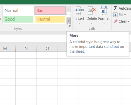
Cell Styles are found on the Home tab of the Excel ribbon, within the Styles command group. 

The Cell Styles command expands to reveal a gallery of Excel-defined cell styles. In some versions of Excel, you have to click the More dropdown button, which is an arrow with a small line at the top.

In Windows systems, hovering over any of these styles will show a preview of the cell’s appearance in the active cell.

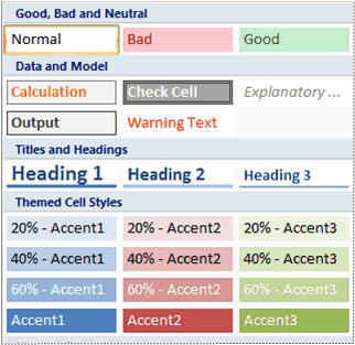
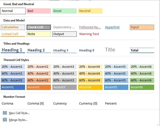
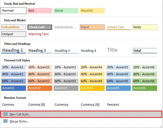
Good, Bad and Neutral

The Good, Bad and Neutral section is usually used to represent each respective data type based on how you want it to be interpreted. Sometimes you want to be able to quickly skim through a document to determine if the values that you are looking at represent a positive or negative outcome.

For example, a higher expense figure is usually considered less favorable, but a higher income figure is considered more favorable. It may be easy to lose track of what you’re looking at without a visual reminder. This section of the Cell Styles gallery accomplishes this.

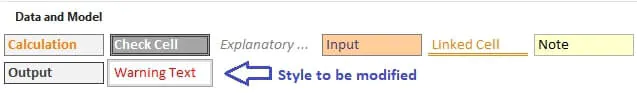
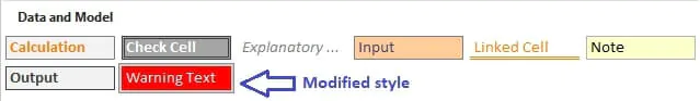
Data and Model

The Data and Model section of the Cell Styles gallery indicates special types of values, including calculated results, cells where users should input values, cells that display output values, and warning cells. 

Titles and Headings

The Titles and Headings section is a quick and easy way to find formatting for title cell styles and different levels of headings according to their importance. A double-underlined Total cell style format is also available in this section.

Themed Cell Styles

The Themed Cell Styles section offers varying degrees of color accents that complement the overall theme of the workbook.

Number Format

In the Number Format section, there are five options for the display style of numbers in the active or selected cell(s) — comma-style with and without decimals, currency-style with and without decimals, and percent-style.

How to create a custom cell style

If you want to create your own cell style in Excel from scratch, click New Cell Style from the Cell Styles dropdown.

This will open up the Style dialog box, where you can overwrite the name in the Style name field to save your custom style with a name you like.

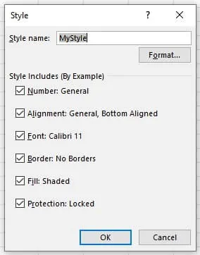
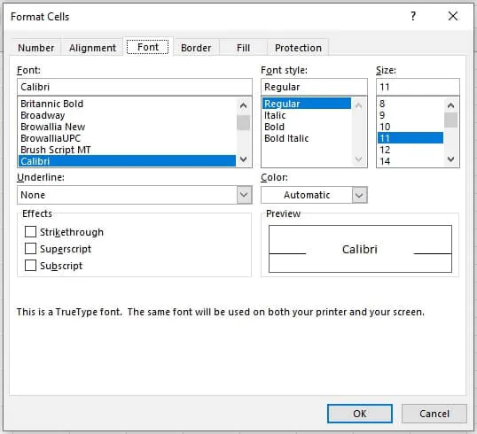
Excel uses the format of the active cell as a starting point for your new cell style. In the example above, our new style is assumed to be 11 point Calibri font with a General number format. To change any of the attributes of the style being created, click on the Format… button. This will open the Format Cells dialog box where you can apply and save Number, Alignment, Font, Border, Fill, and Protection settings. 

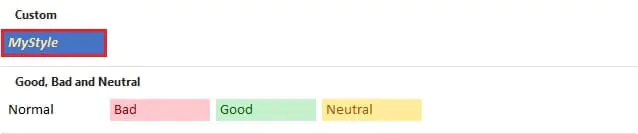
After making the desired changes, click OK from both windows and your custom style will be saved to the Custom section of the Cell Styles gallery, and can now be used anywhere within that workbook.

Create a cell style by modifying an existing cell style

There are two ways to modify an existing cell style.

Method 1 — Duplicate and modify

If there is an existing style that’s almost what you want but not quite, you can treat it as a template and modify it by taking the following steps:

1. Duplicate the existing style by right-clicking on the style from the Cell Styles gallery, then clicking Duplicate.
2. Rename the style in the Style name field
3. Click the Format button, select the elements to apply using the Format Cells window, and click OK.

This will be saved as a new custom style in the Custom section of the Cell Styles dropdown menu.

The original style will still exist in its original location when this method is used.

Method 2 — Modify and overwrite

You can overwrite the format settings on an existing cell style by doing the following: 

1. Right-click on the style name from the Cell Styles gallery and select Modify.
2. Click the Format button, change the elements to be modified using the Format Cells window, and click OK.

The original cell style will carry the same name, but will now carry the formatting features you have just created.

Note that Custom-built cell styles can be modified or renamed, while Excel built-in cell styles can be modified but cannot be renamed. 

Remove a cell style from data

To revert a cell to the default Excel style, select the relevant cell(s) and click the Normal style from the Good, Bad and Neutral section of the Cell Styles gallery.

Delete a predefined or custom cell style

To delete a cell style, right-click on the style name from the Cell Styles gallery and select Delete. You will not get a warning message before this action is taken! Excel will delete that style and will remove the formatting from all cells in that workbook where that style had been applied. 

Merge (import) a cell style from another workbook

You can import built-in or custom cell styles from another workbook by using the Merge Styles command. Both workbooks must be open.

1. Go to the Cell Styles command on the Home tab.
2. Click Merge Styles at the bottom of the dropdown menu
3. From the Merge Styles dialog box, select a workbook that has the style(s) you want to copy to the Destination workbook and click OK.
4. Custom styles from the Source workbook will appear in the Custom section of the Destination workbook, and Excel-defined styles will appear in their respective sections.

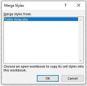
This method is also useful if you deleted a built-in cell style by mistake and want to restore it.

Cell Styles vs. Themes

Cell styles are different from the Themes available on the Page Layout tab. 

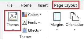
Each theme carries its own font, font size, and color scheme. The options offered in the cell style gallery will change to complement the selected theme and color scheme applied to the workbook. You can shrink the size of the Themes dropdown gallery by dragging on the lower right corner of the window. This will allow you to preview what your document will look like by hovering over the different themes in the gallery.

Liked learning about cell styles in Excel? Here are a few other cool tricks to make your already awesome work look like a masterpiece.

Overview

Starting with Excel 2007, Microsoft enhanced the Excel Cell Styles feature providing great built-in choices and flexibility. The purpose of this post is to briefly discuss the styles feature and demonstrate how it can be used in conjunction with worksheet protection.

Cell Styles

Think of a cell style as a comprehensive set of cell formats, which may include for example the fill color and borders.  Once the style is defined, you can apply the style to the cells, rather than format the cells directly. The beauty of using a style is that the definition of the style is centrally stored in the workbook. When you update the style definition the changes automatically flow out to all cells that use that style.

This is in sharp contrast to the typical way users format cells, which is to apply formatting to the cells directly.  The problem with the traditional approach is when you change your mind and want to update the formatting.  Let’s say you use a yellow fill throughout the workbook to identify user input cells.  If you change your mind about a given format, and want to change the fill from yellow to gray, then you would need to go through each worksheet in the workbook and update all of the individual cells. Depending on the number of sheets and cells involved, this could take a long time.  If, on the other hand, you applied the same cell style to all of those cells, and then changed your mind, you would simply modify the style definition. All cells that use that style would immediately be updated.

Microsoft provides many built-in styles, and you can also create your own, or modify the built-in styles. The built-in style I use most often is the Input cell style, which is sort of a peach color. I use this to highlight all of the input cells in the workbook. This makes it fast and easy for the user of the workbook to know exactly which cells require manual input. This promotes efficiency and reduces errors in the workbook over time.  How so? Well, the user doesn’t need to spend time reviewing all of the cells, trying to determine if they are formula cells or static cells or input cells. Highlighting input cells can also reduce errors in the workbook because it helps minimize the risk of a user accidentally typing over a formula. Of course, this risk could be further minimized with the use of worksheet protection. So, let’s chat about that now.

Worksheet Protection

Worksheet protection protects the cells within a worksheet. Once turned on, the locked attribute of all cells is enforced. What’s that? Yes, once worksheet protection is enabled, the locked attribute is enforced. Let’s unpack that a bit.

You know how you can lock or unlock a cell? There are of course several ways to do this, but for now, let me throw up a screenshot of the Format Cells dialog box, which is activated by going to the Format > Format Cells ribbon command.

There you can see the Locked checkbox on the Protection tab. This tells Excel whether or not to lock the cell.  By default, all cells in all sheets in all books are locked.  What!  Yes, by default, all cells, in all worksheets, in all workbooks are locked. However, the locked attribute is not enforced until worksheet protection is applied. See?

It is pretty easy to turn on worksheet protection, there are several ways, one of which is to click on the Review > Protect Sheet ribbon command.

Once you turn on worksheet protection, the locked attribute is enforced. A locked cell is unable to be edited by the user.

So, now for the big finish, and how this ties back to cell styles.

Styles and Protection

One common task is to unlock certain cells, namely input cells, and then turn on worksheet protection. This results in a worksheet that the user can enter data into, specifically into the unlocked input cells.  The user can’t mess up the formulas or other static values, because they reside in locked cells. Often, I’m asked if there is an automatic way to highlight the unlocked cells.  While there is some conditional formatting that could accomplish this, it is overkill.

In my opinion, the best approach is to highlight the input cells with the Input cell style. By default, the Input cell style does not unlock the cell, in fact, it doesn’t change the locked attribute at all. However, with a quick and easy step, we can modify the Input cell style definition so that when the style is applied it unlocks the cell at the same time. This is perfect, since you highlight the input cells using the Input cell style, and the cells get unlocked at the same time. Then, when you apply worksheet protection, the input cells are automatically unlocked allowing a user to make changes.

To modify the built-in Input cell style so that the locked attribute is applied, simply right-click the Input cell style icon from the Home > Cell Styles ribbon and select Modify… from the shortcut menu.  You’ll be presented with the Style dialog box shown below.

You’ll notice that, by default, the Protection box is unchecked. This means that the style will not override the existing cell protection status. It just leaves it alone. In our use, however, we want to define the protection status (unlocked) and apply it to the cell when we apply the style. Thus, we check the Protection check box and then click the Format button.  On the resulting Format Cells dialog box, we uncheck the Locked checkbox, as shown below

Then, we’ll return to the Style dialog, with the Protection box checked, as shown below.

With the built-in Input cell style now modified, once it is applied to input cells, they will be unlocked and highlighted. And, once we turn on worksheet protection, the cells that use the Input cell style will be identified and unlocked with no extra steps needed.

This is one of my favorite uses of cell styles, and I love how they can integrate so easily with worksheet protection.  Thanks Microsoft!