Cell row number in excel

Date yes Add (Subtract) Days to a Date Concatenate Dates Convert Date to Number Convert Date to Text Month Name to Number Create Date Range from Dates Day Number of Year Month Name from Date First Day of Month Add (Subtract) Weeks to a Date If Functions with Dates Max Date Number of Days Between Dates Number of Days in a Month Number of Weeks Between Dates Number of Years Between Dates Split Date & Time into Separate Cells Countdown Remaining Days Insert Dates Random Date Generator Using Dynamic Ranges — Year to Date Values Add (Subtract) Years to a Date Date Formula Examples Extract Day from Date Get Day Name from Date Count Days Left in Month / Year Count Workdays Left in Month / Year Get Last Day of Month Last Business Day of Month / Year Number of Work / Business Days in Month Weekday Abbreviations Auto Populate Dates Number of Months Between Dates Quarter from a Date Years of Service Change Date Format Compare Dates Time yes Add (Subtract) Hours to Time Add (Subtract) Minutes to Time Add (Subtract) Seconds to Time Add Up time (Total Time) Time Differences Change Time Format Convert Minutes to Hours Convert Time to Decimal Convert Time to Hours Convert Time to Minutes Convert Time to Seconds Military Time Round Time to Nearest 15 Minutes Overtime Calculator Number of Hours Between Times Convert Seconds to Minutes, Hours, or Time Count Hours Worked Time Differences Time Format — Show Minutes Seconds Text yes Add Commas to Cells Get First Word from Text Capitalize First Letter Clean & Format Phone #s Remove Extra Trailing / Leading Spaces Add Spaces to Cell Assign Number Value to Text Combine Cells with Comma Combine First and Last Names Convert Text String to Date Convert Text to Number Extract Text From Cell Get Last Word Remove Unwated Characters Extract Text Before or After Character How to Split Text String by Space, Comma, & More Remove Special Characters Remove First Characters from Left Substitute Multiple Values Switch First & Last Names w/ Commas Remove Specific Text from a Cell Extract Text Between Characters (Ex. Parenthesis) Add Leading Zeros to a Number Remove Line Breaks from Text Remove all Numbers from Text Reverse Text Remove Non-Numeric Characters Remove Last Character(s) From Right Separate First and Last Names Separate Text & Numbers Round yes Round Formulas Round Price to Nearest Dollar or Cent Round to Nearest 10, 100, or 1000 Round to Nearest 5 or .5 Round Percentages Round to Significant Figures Count yes Count Blank and Non-blank Cells Count Cells Between Two Numbers Count Cells not Equal to Count if Cells are in Range Count Times Word Appears in Cell Count Words in Cell Count Specific Characters in Column Count Total Number of Characters in Column Count Cells that Equal one of two Results Count Cells that do not Contain Count Cells that Contain Specific Text Count Unique Values in Range Countif — Multiple Criteria Count Total Number of Cells in Range Count Cells with Any Text Count Total Cells in a Table Lookup yes Two Dimensional VLOOKUP VLOOKUP Simple Example Vlookup — Multiple Matches Case Sensitive Lookup Case Sensitive VLOOKUP Sum if — VLOOKUP Case Sensitive Lookup Case Sensitive VLOOKUP Find Duplicates w/ VLOOKUP or MATCH INDEX MATCH MATCH Lookup — Return Cell Address (Not Value) Lookup Last Value in Column or Row Reverse VLOOKUP (Right to Left) Risk Score Bucket with VLOOKUP Sum with a VLOOKUP Function VLOOKUP & INDIRECT VLOOKUP Concatenate VLOOKUP Contains (Partial Match) 17 Reasons Why Your XLOOKUP is Not Working Double (Nested) XLOOKUP — Dynamic Columns IFERROR (& IFNA) XLOOKUP Lookup Min / Max Value Nested VLOOKUP Top 11 Alternatives to VLOOKUP (Updated 2022!) VLOOKUP – Dynamic Column Reference VLOOKUP – Fix #N/A Error VLOOKUP – Multiple Sheets at Once VLOOKUP & HLOOKUP Combined VLOOKUP & MATCH Combined VLOOKUP Between Worksheets or Spreadsheets VLOOKUP Duplicate Values VLOOKUP Letter Grades VLOOKUP Return Multiple Columns VLOOKUP Returns 0? Return Blank Instead VLOOKUP w/o #N/A Error XLOOKUP Multiple Sheets at Once XLOOKUP Between Worksheets or Spreadsheets XLOOKUP by Date XLOOKUP Duplicate Values XLOOKUP Multiple Criteria XLOOKUP Return Multiple Columns XLOOKUP Returns 0? Return Blank Instead XLOOKUP Text XLOOKUP with IF XLOOKUP With If Statement Misc. yes Sort Multiple Columns Use Cell Value in Formula Percentage Change Between Numbers Percentage Breakdown Rank Values Add Spaces to Cell CAGR Formula Average Time Decimal Part of Number Integer Part of a Number Compare Items in a List Dealing with NA() Errors Get Worksheet Name Wildcard Characters Hyperlink to Current Folder Compound Interest Formula Percentage Increase Create Random Groups Sort with the Small and Large Functions Non-volatile Function Alternatives Decrease a Number by a Percentage Calculate Percent Variance Profit Margin Calculator Convert Column Number to Letter Get Full Address of Named Range Insert File Name Insert Path Latitute / Longitude Functions Replace Negative Values Reverse List Range Convert State Name to Abbreviation Create Dynamic Hyperlinks Custom Sort List with Formula Data Validation — Custom Formulas Dynamic Sheet Reference (INDIRECT) Reference Cell in Another Sheet or Workbook Get Cell Value by Address Get Worksheet Name Increment Cell Reference List Sheet Names List Skipped Numbers in Sequence Return Address of Max Value in Range Search by Keywords Select Every Other (or Every nth) Row Basics yes Cell Reference Basics — A1, R1C1, 3d, etc. Add Up (Sum) Entire Column or Row Into to Dynamic Array Formulas Conversions yes Convert Time Zones Convert Celsius to Fahrenheit Convert Pounds to Kilograms Convert Time to Unix Time Convert Feet to Meters Convert Centimeters to Inches Convert Kilometers to Miles Convert Inches to Feet Convert Date to Julian Format Convert Column Letter to Number Tests yes Test if a Range Contains any Text Test if any Cell in Range is Number Test if a Cell Contains a Specific Value Test if Cell Contains Any Number Test if Cell Contains Specific Number Test if Cell is Number or Text If yes Percentile If Subtotal If Sumproduct If Large If and Small If Median If Concatentate If Max If Rank If TEXTJOIN If Sum yes Sum if — Begins With / Ends With Sum if — Month or Year to Date Sum if — By Year Sum if — Blank / Non-Blank Sum if — Horizontal Sum Count / Sum If — Cell Color INDIRECT Sum Sum If — Across Multiple Sheets Sum If — By Month Sum If — Cells Not Equal To Sum If — Not Blank Sum if — Between Values Sum If — Week Number Sum Text Sum if — By Category or Group Sum if — Cell Contains Specific Text (Wildcards) Sum if — Date Rnage Sum if — Dates Equal Sum if — Day of Week Sum if — Greater Than Sum if — Less Than Average yes Average Non-Zero Values Average If — Not Blank Average — Ignore 0 Average — Ignore Errors Math yes Multiplication Table Cube Roots nth Roots Square Numbers Square Roots Calculations yes Calculate a Ratio Calculate Age KILLLLLLL Calculate Loan Payments GPA Formula Calculate VAT Tax How to Grade Formulas Find yes Find a Number in a Column / Workbook Find Most Frequent Numbers Find Smallest n Values Find nth Occurance of Character in Text Find and Extract Number from String Find Earliest or Latest Date Based on Criteria Find First Cell with Any Value Find Last Row Find Last Row with Data Find Missing Values Find Largest n Values Most Frequent Number Conditional Formatting yes Conditional Format — Dates & Times Conditional Format — Highlight Blank Cells New Functions XLOOKUP Replaces VLOOKUP, HLOOKUP, and INDEX / MATCH Logical yes AND Checks whether all conditions are met. TRUE/FALSE IF If condition is met, do something, if not, do something else. IFERROR If result is an error then do something else. NOT Changes TRUE to FALSE and FALSE to TRUE. OR Checks whether any conditions are met. TRUE/FALSE XOR Checks whether one and only one condition is met. TRUE/FALSE Lookup & Reference yes FALSE The logical value: FALSE. TRUE The logical value: TRUE. ADDRESS Returns a cell address as text. AREAS Returns the number of areas in a reference. CHOOSE Chooses a value from a list based on it’s position number. COLUMN Returns the column number of a cell reference. COLUMNS Returns the number of columns in an array. HLOOKUP Lookup a value in the first row and return a value. HYPERLINK Creates a clickable link. INDEX Returns a value based on it’s column and row numbers. INDIRECT Creates a cell reference from text. LOOKUP Looks up values either horizontally or vertically. MATCH Searches for a value in a list and returns its position. OFFSET Creates a reference offset from a starting point. ROW Returns the row number of a cell reference. ROWS Returns the number of rows in an array. TRANSPOSE Flips the oriention of a range of cells. VLOOKUP Lookup a value in the first column and return a value. Date & Time yes DATE Returns a date from year, month, and day. DATEDIF Number of days, months or years between two dates. DATEVALUE Converts a date stored as text into a valid date DAY Returns the day as a number (1-31). DAYS Returns the number of days between two dates. DAYS360 Returns days between 2 dates in a 360 day year. EDATE Returns a date, n months away from a start date. EOMONTH Returns the last day of the month, n months away date. HOUR Returns the hour as a number (0-23). MINUTE Returns the minute as a number (0-59). MONTH Returns the month as a number (1-12). NETWORKDAYS Number of working days between 2 dates. NETWORKDAYS.INTL Working days between 2 dates, custom weekends. NOW Returns the current date and time. SECOND Returns the second as a number (0-59) TIME Returns the time from a hour, minute, and second. TIMEVALUE Converts a time stored as text into a valid time. TODAY Returns the current date. WEEKDAY Returns the day of the week as a number (1-7). WEEKNUM Returns the week number in a year (1-52). WORKDAY The date n working days from a date. WORKDAY.INTL The date n working days from a date, custom weekends. YEAR Returns the year. YEARFRAC Returns the fraction of a year between 2 dates. Engineering yes CONVERT Convert number from one unit to another. Financial yes FV Calculates the future value. PV Calculates the present value. NPER Calculates the total number of payment periods. PMT Calculates the payment amount. RATE Calculates the interest Rate. NPV Calculates the net present value. IRR The internal rate of return for a set of periodic CFs. XIRR The internal rate of return for a set of non-periodic CFs. PRICE Calculates the price of a bond. YIELD Calculates the bond yield. INTRATE The interest rate of a fully invested security. Information yes CELL Returns information about a cell. ERROR.TYPE Returns a value representing the cell error. ISBLANK Test if cell is blank. TRUE/FALSE ISERR Test if cell value is an error, ignores #N/A. TRUE/FALSE ISERROR Test if cell value is an error. TRUE/FALSE ISEVEN Test if cell value is even. TRUE/FALSE ISFORMULA Test if cell is a formula. TRUE/FALSE ISLOGICAL Test if cell is logical (TRUE or FALSE). TRUE/FALSE ISNA Test if cell value is #N/A. TRUE/FALSE ISNONTEXT Test if cell is not text (blank cells are not text). TRUE/FALSE ISNUMBER Test if cell is a number. TRUE/FALSE ISODD Test if cell value is odd. TRUE/FALSE ISREF Test if cell value is a reference. TRUE/FALSE ISTEXT Test if cell is text. TRUE/FALSE N Converts a value to a number. NA Returns the error: #N/A. TYPE Returns the type of value in a cell. Math yes ABS Calculates the absolute value of a number. AGGREGATE Define and perform calculations for a database or a list. CEILING Rounds a number up, to the nearest specified multiple. COS Returns the cosine of an angle. DEGREES Converts radians to degrees. DSUM Sums database records that meet certain criteria. EVEN Rounds to the nearest even integer. EXP Calculates the exponential value for a given number. FACT Returns the factorial. FLOOR Rounds a number down, to the nearest specified multiple. GCD Returns the greatest common divisor. INT Rounds a number down to the nearest integer. LCM Returns the least common multiple. LN Returns the natural logarithm of a number. LOG Returns the logarithm of a number to a specified base. LOG10 Returns the base-10 logarithm of a number. MOD Returns the remainder after dividing. MROUND Rounds a number to a specified multiple. ODD Rounds to the nearest odd integer. PI The value of PI. POWER Calculates a number raised to a power. PRODUCT Multiplies an array of numbers. QUOTIENT Returns the integer result of division. RADIANS Converts an angle into radians. RAND Calculates a random number between 0 and 1. RANDBETWEEN Calculates a random number between two numbers. ROUND Rounds a number to a specified number of digits. ROUNDDOWN Rounds a number down (towards zero). ROUNDUP Rounds a number up (away from zero). SIGN Returns the sign of a number. SIN Returns the sine of an angle. SQRT Calculates the square root of a number. SUBTOTAL Returns a summary statistic for a series of data. SUM Adds numbers together. SUMIF Sums numbers that meet a criteria. SUMIFS Sums numbers that meet multiple criteria. SUMPRODUCT Multiplies arrays of numbers and sums the resultant array. TAN Returns the tangent of an angle. TRUNC Truncates a number to a specific number of digits. Stats yes AVERAGE Averages numbers. AVERAGEA Averages numbers. Includes text & FALSE =0, TRUE =1. AVERAGEIF Averages numbers that meet a criteria. AVERAGEIFS Averages numbers that meet multiple criteria. CORREL Calculates the correlation of two series. COUNT Counts cells that contain a number. COUNTA Count cells that are non-blank. COUNTBLANK Counts cells that are blank. COUNTIF Counts cells that meet a criteria. COUNTIFS Counts cells that meet multiple criteria. FORECAST Predict future y-values from linear trend line. FREQUENCY Counts values that fall within specified ranges. GROWTH Calculates Y values based on exponential growth. INTERCEPT Calculates the Y intercept for a best-fit line. LARGE Returns the kth largest value. LINEST Returns statistics about a trendline. MAX Returns the largest number. MEDIAN Returns the median number. MIN Returns the smallest number. MODE Returns the most common number. PERCENTILE Returns the kth percentile. PERCENTILE.INC Returns the kth percentile. Where k is inclusive. PERCENTILE.EXC Returns the kth percentile. Where k is exclusive. QUARTILE Returns the specified quartile value. QUARTILE.INC Returns the specified quartile value. Inclusive. QUARTILE.EXC Returns the specified quartile value. Exclusive. RANK Rank of a number within a series. RANK.AVG Rank of a number within a series. Averages. RANK.EQ Rank of a number within a series. Top Rank. SLOPE Calculates the slope from linear regression. SMALL Returns the kth smallest value. STDEV Calculates the standard deviation. STDEV.P Calculates the SD of an entire population. STDEV.S Calculates the SD of a sample. STDEVP Calculates the SD of an entire population TREND Calculates Y values based on a trendline. Text yes CHAR Returns a character specified by a code. CLEAN Removes all non-printable characters. CODE Returns the numeric code for a character. CONCATENATE Combines text together. DOLLAR Converts a number to text in currency format. EXACT Test if cells are exactly equal. Case-sensitive. TRUE/FALSE FIND Locates position of text within a cell.Case-sensitive. LEFT Truncates text a number of characters from the left. LEN Counts number of characters in text. LOWER Converts text to lower case. MID Extracts text from the middle of a cell. PROPER Converts text to proper case. REPLACE Replaces text based on it’s location. REPT Repeats text a number of times. RIGHT Truncates text a number of characters from the right. SEARCH Locates position of text within a cell.Not Case-sensitive. SUBSTITUTE Finds and replaces text. Case-sensitive. TEXT Converts a value into text with a specific number format. TRIM Removes all extra spaces from text. UPPER Converts text to upper case. VALUE Converts a number stored as text into a number.

How to get the row or column number of the current cell or any other cell in Excel.

This tutorial covers important functions that allow you to do everything from alternate row and column shading to incrementing values at specified intervals and much more.

We will use the ROW and COLUMN function for this.  Here is an example of the output from these functions.

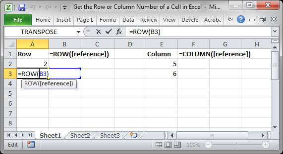
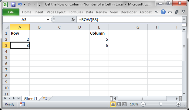
Though this doesn’t look like much, these functions allow for the creation of powerful formulas when combined with other functions.  Now, let’s look at how to create them.

Get a Cell’s Row Number

Syntax

This function returns the number of the row that a particular cell is in.

If you leave the function empty, it will return the row number for the current cell in which this function has been placed.

If you put a cell reference within this function, it will return the row number for that cell reference.

This example would return 1 since cell A1 is in row 1.  If it was =ROW(C24) the function would return the number 24 because cell C24 is in row 24.

Examples

Now that you know how this function works, it may seem rather useless.  Here are links to two examples where this function is key.

Increment a Value Every X Number of Rows in Excel

Shade Every Other Row in Excel Quickly

Get a Cell’s Column Number

Syntax

This function returns the number of the column that a particular cell is in.  It counts from left to right, where A is 1 and B is 2 and so on.

If you leave the function empty, it will return the column number for the current cell in which this function has been placed.

If you put a cell reference within this function, it will return the column number for that cell reference.

This example would return 1 since cell A1 is in row 1.  If it was =COLUMN (C24) the function would return the number 3 because cell C24 is in column number 3.

Examples

The COLUMN function works just like the ROW function does except that it works on columns, going left to right, whereas the ROW function works on rows, going up and down.

As such, almost every example where ROW is used could be converted to use COLUMN based on your needs.

Notes

The ROW and COLUMN functions are building blocks in that they help you create more complex formulas in Excel.  Alone, these functions are pretty much worthless, but, if you can memorize them and keep them for later, you will start to find more and more uses for them when working in large data sets.  The examples provided above in the ROW section cover only two of many different ways you can use these functions to create more powerful and helpful spreadsheets.

Similar Content on TeachExcel

Sum Values from Every X Number of Rows in Excel

Tutorial: Add values from every x number of rows in Excel. For instance, add together every other va…

Formulas to Remove First or Last Character from a Cell in Excel

Tutorial: Formulas that allow you to quickly and easily remove the first or last character from a ce…

Formula to Delete the First or Last Word from a Cell in Excel

Tutorial:
Excel formula to delete the first or last word from a cell.
You can copy and paste the fo…

Reverse the Contents of a Cell in Excel — UDF

Macro: Reverse cell contents with this free Excel UDF (user defined function). This will mir…

Excel Function to Remove All Text OR All Numbers from a Cell

Tutorial: How to create and use a function that removes all text or all numbers from a cell, whichev…

Get the First Word from a Cell in Excel

Tutorial: How to use a formula to get the first word from a cell in Excel. This works for a single c…

Subscribe for Weekly Tutorials

BONUS: subscribe now to download our Top Tutorials Ebook!

Watch Video – 7 Quick and Easy Ways to Number Rows in Excel

When working with Excel, there are some small tasks that need to be done quite often. Knowing the ‘right way’ can save you a great deal of time.

One such simple (yet often needed) task is to number the rows of a dataset in Excel (also called the serial numbers in a dataset).

How to Number Rows in Excel - Example dataset

Now if you’re thinking that one of the ways is to simply enter these serial number manually, well – you’re right!

But that’s not the best way to do it.

Imagine having hundreds or thousands of rows for which you need to enter the row number. It would be tedious – and completely unnecessary.

There are many ways to number rows in Excel, and in this tutorial, I am going to share some of the ways that I recommend and often use.

Of course, there would be more, and I will be waiting – with a coffee – in the comments area to hear from you about it.

How to Number Rows in Excel

The best way to number the rows in Excel would depend on the kind of data set that you have.

For example, you may have a continuous data set that starts from row 1, or a dataset that start from a different row. Or, you might have a dataset that has a few blank rows in it, and you only want to number the rows that are filled.

You can choose any one of the methods that work based on your dataset.

1] Using Fill Handle

Fill handle identifies a pattern from a few filled cells and can easily be used to quickly fill the entire column.

Suppose you have a dataset as shown below:

How to Number Rows in Excel - Dataset

Here are the steps to quickly number the rows using the fill handle:

Note that Fill Handle automatically identifies the pattern and fill the remaining cells with that pattern. In this case, the pattern was that the numbers were getting incrementing by 1.

In case you have a blank row in the dataset, fill handle would only work till the last contiguous non-blank row.

Also, note that in case you don’t have data in the adjacent column, double-clicking the fill handle would not work. You can, however, place the cursor on the fill handle, hold the right mouse key and drag down. It will fill the cells covered by the cursor dragging.

2] Using Fill Series

While Fill Handle is a quick way to number rows in Excel, Fill Series gives you a lot more control over how the numbers are entered.

Suppose you have a dataset as shown below:

How to Number Rows in Excel - Dataset

Here are the steps to use Fill Series to number rows in Excel:

This will instantly number the rows from 1 to 26.

Using ‘Fill Series’ can be useful when you’re starting by entering the row numbers. Unlike Fill Handle, it doesn’t require the adjacent columns to be filled already.

Even if you have nothing on the worksheet, Fill Series would still work.

Note: In case you have blank rows in the middle of the dataset, Fill Series would still fill the number for that row.

3] Using the ROW Function

You can also use Excel functions to number the rows in Excel.

In the Fill Handle and Fill Series methods above, the serial number inserted is a static value. This means that if you move the row (or cut and paste it somewhere else in the dataset), the row numbering will not change accordingly.

This shortcoming can be tackled using formulas in Excel.

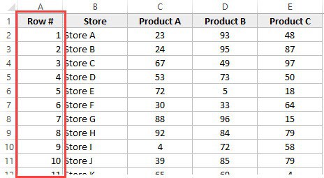
You can use the ROW function to get the row numbering in Excel.

To get the row numbering using the ROW function, enter the following formula in the first cell and copy for all the other cells:

=ROW()-1

The ROW() function gives the row number of the current row. So I have subtracted 1 from it as I started from the second row onwards. If your data starts from the 5th row, you need to use the formula =ROW()-4.

ROW formula to enter row numbers in Excel

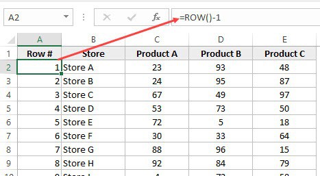
The best part about using the ROW function is that it will not screw up the numberings if you delete a row in your dataset.

Since the ROW function is not referencing any cell, it will automatically (or should I say AutoMagically) adjust to give you the correct row number. Something as shown below:

Automatically number rows in Excel when a row is deleted

Note that as soon as I delete a row, the row numbers automatically update.

Again, this would not take into account any blank records in the dataset. In case you have blank rows, it will still show the row number.

You can use the following formula to hide the row number for blank rows, but it would still not adjust the row numbers (such that the next row number is assigned to the next filled row).

IF(ISBLANK(B2),"",ROW()-1)

4] Using the COUNTA Function

If you want to number rows in a way that only the ones that are filled get a serial number, then this method is the way to go.

It uses the COUNTA function that counts the number of cells in a range that are not empty.

Suppose you have a dataset as shown below:

Number rows in Excel - Using COUNTA function to insert serial numbers

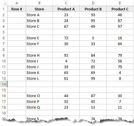
Note that there are blank rows in the above-shown dataset.

Here is the formula that will number the rows without numbering the blank rows.

=IF(ISBLANK(B2),"",COUNTA($B$2:B2))

The IF function checks whether the adjacent cell in column B is empty or not. If it’s empty, it returns a blank, but if it’s not, it returns the count of all the filled cells till that cell.

5] Using SUBTOTAL For Filtered Data

Sometimes, you may have a huge dataset, where you want to filter the data and then copy and paste the filtered data into a separate sheet.

If you use any of the methods shown above so far, you will notice that the row numbers remain the same. This means that when you copy the filtered data, you will have to update the row numbering.

In such cases, the SUBTOTAL function can automatically update the row numbers. Even when you filter the data set, the row numbers will remain intact.

Let me show you exactly how it works with an example.

Suppose you have a dataset as shown below:

Data set for SUBTOTAL functon - insert serial numbers in Excel

If I filter this data based on Product A sales, you will get something as shown below:

Filtered Data row numbers

Note that the serial numbers in Column A are also filtered. So now, you only see the numbers for the rows that are visible.

While this is the expected behavior, in case you want to get a serial row numbering – so that you can simply copy and paste this data somewhere else – you can use the SUBTOTAL function.

Here is the SUBTOTAL function that will make sure that even the filtered data has continuous row numbering.

=SUBTOTAL(3,$B$2:B2)

The 3 in the SUBTOTAL function specifies using the COUNTA function. The second argument is the range on which COUNTA function is applied.

The benefit of the SUBTOTAL function is that it dynamically updates when you filter the data (as shown below):

Subtotal automatically numbers rows in Excel when filtered

Note that even when the data is filtered, the row numbering update and remains continuous.

6] Creating an Excel Table

Excel Table is a great tool that you must use when working with tabular data. It makes managing and using data a lot easier.

This is also my favorite method among all the techniques shown in this tutorial.

Let me first show you the right way to number the rows using an Excel Table:

Number Rows in Excel - Calculated Column in Excel table

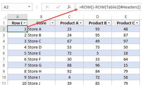
Note that in the formula above, I have used Table2, as that is the name of my Excel table. You can replace Table2 with the name of the table you have.

There are some added benefits of using an Excel Table while numbering rows in Excel:

  1. Since Excel Table automatically inserts the formula in the entire column, it works when you insert a new row in the Table. This means that when you insert/delete rows in an Excel Table, the row numbering would automatically update (as shown below).Inserting Row Numbers in an Excel Table
  2. If you add more rows to the data, Excel Table would automatically expand to include this data as a part of the table. And since the formulas automatically update in the calculated columns, it would insert the row number for the newly inserted row (as shown below).Excel Table - Automatically Add row Number on adding a row

7] Adding 1 to the Previous Row Number

This is a simple method that works.

The idea is to add 1 to the previous row number (the number in the cell above). This will make sure that subsequent rows get a number that is incremented by 1.

Suppose you have a dataset as shown below:

How to Number Rows in Excel - Dataset

Here are the steps to enter row numbers using this method:

  • In the cell in the first row, enter 1 manually. In this case, it’s in cell A2.
  • In cell A3, enter the formula, =A2+1
  • Copy and paste the formula for all the cells in the column.

Add 1 to insert row numbers in Excel

The above steps would enter serial numbers in all the cells in the column. In case there are any blank rows, this would still insert the row number for it.

Also note that in case you insert a new row, the row number would not update. In case you delete a row, all the cells below the deleted row would show a reference error.

These are some quick ways you can use to insert serial numbers in tabular data in Excel.

In case you are using any other method, do share it with me in the comments section.

You May Also Like the Following Excel Tutorials:

  • Delete Blank Rows in Excel (with and without VBA).
  • How to Insert Multiple Rows in Excel (4 Methods).
  • How to Split Multiple Lines in a Cell into a Separate Cells / Columns.
  • 7 Amazing Things Excel Text to Columns Can Do For You.
  • Highlight EVERY Other ROW in Excel.
  • How to Compare Two Columns in Excel.
  • Insert New Columns in Excel

Excel for Microsoft 365 Excel for Microsoft 365 for Mac Excel for the web Excel 2021 Excel 2021 for Mac Excel 2019 Excel 2019 for Mac Excel 2016 Excel 2016 for Mac Excel 2013 Excel 2010 Excel 2007 Excel for Mac 2011 Excel Starter 2010 More…Less

This article describes the formula syntax and usage of the ROW function in Microsoft Excel.

Description

Returns the row number of a reference.

Syntax

ROW([reference])

The ROW function syntax has the following arguments:

  • Reference    Optional. The cell or range of cells for which you want the row number.

    • If reference is omitted, it is assumed to be the reference of the cell in which the ROW function appears.

    • If reference is a range of cells, and if ROW is entered as a vertical array, ROW returns the row numbers of reference as a vertical array.

    • Reference cannot refer to multiple areas.

Examples

Copy the example data in the following table, and paste it in cell A1 of a new Excel worksheet. For formulas to show results, select them, press F2, and then press Enter. If you need to, you can adjust the column widths to see all the data.

Formula

Description

Result

=ROW()

Row in which the formula appears

2

=ROW(C10)

Row of the reference

10

Need more help?

Just like the COLUMN function, the ROW function in Excel is also an important cell reference function in excel.

This tutorial focuses on everything that you need to know about the ROW formula in excel. This blog covers the purpose of the ROW excel formula, its syntax, argument, and examples.

Table of Contents

  1. What is Use of ROW Function in Excel
  2. Syntax and Argument
  3. Examples of ROW Formula in Excel
    1. Using ROW Function (without argument)
    2. Using ROW Formula (with argument)
    3. Practical Usable of ROW Formula

Here we go 😎

What is Use of ROW Function in Excel

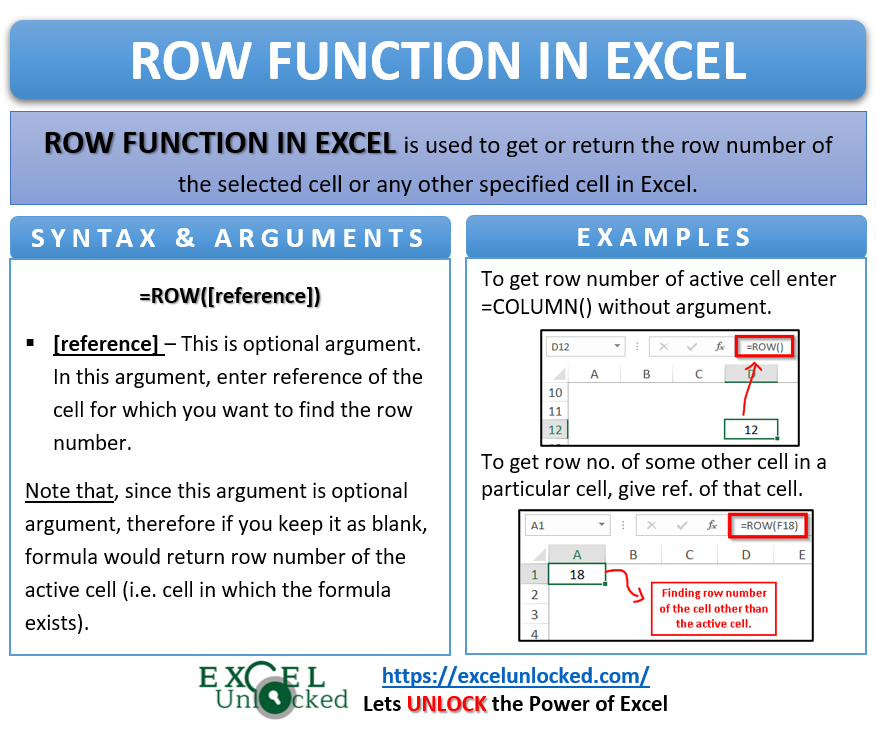
By using the excel ROW function, you can find and get the row number of the selected and active cell or any other cell reference.

The ROW excel formula returns a whole number as its result (i.e. 1, 2, 3, 4, …).

Syntax and Argument

=ROW([reference])

As seen above, the ROW formula in excel has one optional input argument viz [reference].

  • [reference] – This is the optional argument in which you need to enter the reference of the cell for which you want to find the row number.

If you keep the input argument of the ROW function as blank, excel would find and return the row number of the cell in which you are entering the =ROW() formula.

Examples of ROW Formula in Excel

In this section of the blog, we would go through both the types of examples of the ROW formula – i.e. with empty parenthesis and with cell reference.

Using ROW Function (without argument)

As mentioned in the above section, the input argument of the ROW function is an optional argument. It means that if you keep the formula parenthesis as empty, excel finds and returns the row number of the cell in which the formula resides.

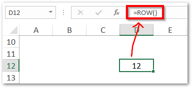
Try entering this formula in cell D12.

=ROW()

As a result, you would notice that excel returns the whole number 12. This is because the row number of active cell D12 is 12.

ROW Function Example Without Input Argument

Let us now consider another example by using the formula input argument.

Infographic - ROW Formula Function in Excel

Using ROW Formula (with argument)

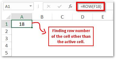
To get the row number of the cell other than the active or selected cell, simply put the cell reference inside the ROW function parenthesis.

Suppose, we want to get or return the row number of the cell $F$18 in cell A1. Use this formula-

=ROW(F18) or =ROW($F$18)

ROW Function Example With Input Argument

Now, when you are clear about how to use the ROW function in excel with and without input argument, let us consider some practical applicability of this formula.

Practical Usable of ROW Formula

In practical projects, I generally use this function to get and return the sequence or the serial number of the table, like this:
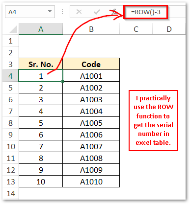
Practical Usage of Excel Row Function

=ROW()-3

In the above examples, the ROW() portion of the above formula returns the row number of selected cell A4 (i.e. 4). And then 3 is deducted from the result of the ROW() portion in order to nullify the impact of blanks rows 1, 2, and 3.

RELATED POSTS

  • CELL Function in Excel – Get Information About Cell

  • ADDRESS Function in Excel – Get Excel Cell Address

  • N Function in Excel – Usage and Examples

  • ISREF Function in Excel – Checking for Cell Reference

  • COLUMNS Function in Excel – Get Number of Columns

  • OFFSET Function in Excel – Jump Rows and Columns

Понравилась статья? Поделить с друзьями:
  • Cell links in excel
  • Cell is not moving in excel
  • Cell indexing in excel
  • Cell in excel will not calculate
  • Cell in excel not updating