
Excel for Microsoft 365 Excel for the web Excel 2021 Excel 2019 Excel 2016 Excel 2013 Excel 2010 Excel 2007 More…Less
A cell reference refers to a cell or a range of cells on a worksheet and can be used in a formula so that Microsoft Office Excel can find the values or data that you want that formula to calculate.
In one or several formulas, you can use a cell reference to refer to:
-
Data from one or more contiguous cells on the worksheet.
-
Data contained in different areas of a worksheet.
-
Data on other worksheets in the same workbook.
For example:
|
This formula: |
Refers to: |
And Returns: |
|---|---|---|
|
=C2 |
Cell C2 |
The value in cell C2. |
|
=A1:F4 |
Cells A1 through F4 |
The values in all cells, but you must press Ctrl+Shift+Enter after you type in your formula. Note: This functionality doesn’t work in Excel for the web. |
|
=Asset-Liability |
The cells named Asset and Liability |
The value in the cell named Liability subtracted from the value in the cell named Asset. |
|
{=Week1+Week2} |
The cell ranges named Week1 and Week2 |
The sum of the values of the cell ranges named Week1 and Week 2 as an array formula. |
|
=Sheet2!B2 |
Cell B2 on Sheet2 |
The value in cell B2 on Sheet2. |
-
Click the cell in which you want to enter the formula.
-
In the formula bar
 , type = (equal sign).
 -
Do one of the following:
-
Reference one or more cells To create a reference, select a cell or range of cells on the same worksheet.
You can drag the border of the cell selection to move the selection, or drag the corner of the border to expand the selection.
-
Reference a defined name To create a reference to a defined name, do one of the following:
-
Type the name.
-
Press F3, select the name in the Paste name box, and then click OK.
Note: If there is no square corner on a color-coded border, the reference is to a named range.
-
-
-
Do one of the following:
-
If you are creating a reference in a single cell, press Enter.
-
If you are creating a reference in an array formula (such A1:G4), press Ctrl+Shift+Enter.
The reference can be a single cell or a range of cells, and the array formula can be one that calculates single or multiple results.
Note: If you have a current version of Microsoft 365, then you can simply enter the formula in the top-left-cell of the output range, then press ENTER to confirm the formula as a dynamic array formula. Otherwise, the formula must be entered as a legacy array formula by first selecting the output range, entering the formula in the top-left-cell of the output range, and then pressing CTRL+SHIFT+ENTER to confirm it. Excel inserts curly brackets at the beginning and end of the formula for you. For more information on array formulas, see Guidelines and examples of array formulas.
-
 , type = (equal sign).
You can refer to cells that are on other worksheets in the same workbook by prepending the name of the worksheet followed by an exclamation point (!) to the start of the cell reference. In the following example, the worksheet function named AVERAGE calculates the average value for the range B1:B10 on the worksheet named Marketing in the same workbook.

1. Refers to the worksheet named Marketing
2. Refers to the range of cells between B1 and B10, inclusively
3. Separates the worksheet reference from the cell range reference
-
Click the cell in which you want to enter the formula.
-
In the formula bar
, type = (equal sign) and the formula you want to use. -
Click the tab for the worksheet to be referenced.
-
Select the cell or range of cells to be referenced.
Note: If the name of the other worksheet contains nonalphabetical characters, you must enclose the name (or the path) within single quotation marks (‘).
Alternatively, you can copy and paste a cell reference and then use the Link Cells command to create a cell reference. You can use this command to:
-
Easily display important information in a more prominent position. Let’s say that you have a workbook that contains many worksheets, and on each worksheet is a cell that displays summary information about the other cells on that worksheet. To make these summary cells more prominent, you can create a cell reference to them on the first worksheet of the workbook, which enables you to see summary information about the whole workbook on the first worksheet.
-
Make it easier to create cell references between worksheets and workbooks. The Link Cells command automatically pastes the correct syntax for you.
-
Click the cell that contains the data you want to link to.
-
Press Ctrl+C, or go to the Home tab, and in the Clipboard group, click Copy
.
-
Press Ctrl+V, or go to the Home tab, in the Clipboard group, click Paste
.By default, the Paste Options
button appears when you paste copied data. -
Click the Paste Options button, and then click Paste Link
.
 .
.
 .
. button appears when you paste copied data.
 .
.-
Double-click the cell that contains the formula that you want to change. Excel highlights each cell or range of cells referenced by the formula with a different color.
-
Do one of the following:
-
To move a cell or range reference to a different cell or range, drag the color-coded border of the cell or range to the new cell or range.
-
To include more or fewer cells in a reference, drag a corner of the border.
-
In the formula bar
, select the reference in the formula, and then type a new reference. -
Press F3, select the name in the Paste name box, and then click OK.
-
-
Press Enter, or, for an array formula, press Ctrl+Shift+Enter.
Note: If you have a current version of Microsoft 365, then you can simply enter the formula in the top-left-cell of the output range, then press ENTER to confirm the formula as a dynamic array formula. Otherwise, the formula must be entered as a legacy array formula by first selecting the output range, entering the formula in the top-left-cell of the output range, and then pressing CTRL+SHIFT+ENTER to confirm it. Excel inserts curly brackets at the beginning and end of the formula for you. For more information on array formulas, see Guidelines and examples of array formulas.
Frequently, if you define a name to a cell reference after you enter a cell reference in a formula, you may want to update the existing cell references to the defined names.
-
Do one of the following:
-
Select the range of cells that contains formulas in which you want to replace cell references with defined names.
-
Select a single, empty cell to change the references to names in all formulas on the worksheet.
-
-
On the Formulas tab, in the Defined Names group, click the arrow next to Define Name, and then click Apply Names.
-
In the Apply names box, click one or more names, and then click OK.
-
Select the cell that contains the formula.
-
In the formula bar
, select the reference that you want to change. -
Press F4 to switch between the reference types.
For more information about the different type of cell references, see Overview of formulas.
-
Click the cell in which you want to enter the formula.
-
In the formula bar
, type = (equal sign). -
Select a cell or range of cells on the same worksheet. You can drag the border of the cell selection to move the selection, or drag the corner of the border to expand the selection.
-
Do one of the following:
-
If you are creating a reference in a single cell, press Enter.
-
If you are creating a reference in an array formula (such A1:G4), press Ctrl+Shift+Enter.
The reference can be a single cell or a range of cells, and the array formula can be one that calculates single or multiple results.
Note: If you have a current version of Microsoft 365, then you can simply enter the formula in the top-left-cell of the output range, then press ENTER to confirm the formula as a dynamic array formula. Otherwise, the formula must be entered as a legacy array formula by first selecting the output range, entering the formula in the top-left-cell of the output range, and then pressing CTRL+SHIFT+ENTER to confirm it. Excel inserts curly brackets at the beginning and end of the formula for you. For more information on array formulas, see Guidelines and examples of array formulas.
-
You can refer to cells that are on other worksheets in the same workbook by prepending the name of the worksheet followed by an exclamation point (!) to the start of the cell reference. In the following example, the worksheet function named AVERAGE calculates the average value for the range B1:B10 on the worksheet named Marketing in the same workbook.
1. Refers to the worksheet named Marketing
2. Refers to the range of cells between B1 and B10, inclusively
3. Separates the worksheet reference from the cell range reference
-
Click the cell in which you want to enter the formula.
-
In the formula bar
, type = (equal sign) and the formula you want to use. -
Click the tab for the worksheet to be referenced.
-
Select the cell or range of cells to be referenced.
Note: If the name of the other worksheet contains nonalphabetical characters, you must enclose the name (or the path) within single quotation marks (‘).
-
Double-click the cell that contains the formula that you want to change. Excel highlights each cell or range of cells referenced by the formula with a different color.
-
Do one of the following:
-
To move a cell or range reference to a different cell or range, drag the color-coded border of the cell or range to the new cell or range.
-
To include more or fewer cells in a reference, drag a corner of the border.
-
In the formula bar
, select the reference in the formula, and then type a new reference.
-
-
Press Enter, or, for an array formula, press Ctrl+Shift+Enter.
Note: If you have a current version of Microsoft 365, then you can simply enter the formula in the top-left-cell of the output range, then press ENTER to confirm the formula as a dynamic array formula. Otherwise, the formula must be entered as a legacy array formula by first selecting the output range, entering the formula in the top-left-cell of the output range, and then pressing CTRL+SHIFT+ENTER to confirm it. Excel inserts curly brackets at the beginning and end of the formula for you. For more information on array formulas, see Guidelines and examples of array formulas.
-
Select the cell that contains the formula.
-
In the formula bar
, select the reference that you want to change. -
Press F4 to switch between the reference types.
For more information about the different type of cell references, see Overview of formulas.
Need more help?
You can always ask an expert in the Excel Tech Community or get support in the Answers community.
Need more help?
Microsoft Excel, sometimes known as MS Excel, is a potent spreadsheet programme. In Excel, each worksheet consists of a number of cells that are made up of rows and columns. Each cell has a unique reference, which enables users to quickly access and address the required cell (or cells) within the functions. In Excel, cell references are crucial, particularly when working with huge data sets in functions and formulas.
This article covers a quick overview of Excel Cell References. The various sorts of cell references that Excel offers and the detailed instructions for using each one are also covered in the article.
What is a Cell Reference?
An Excel cell reference, also known as a cell address, is a mechanism that defines a cell on a worksheet by combining a column letter and a row number. We can refer to any cell (in Excel formulas) in the worksheet by using the cell references.
For example:
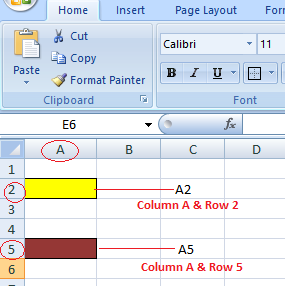
Here we refer to the cell in column A & row 2 by A2 & cell in column A & row 5 by A5. You can make use of such notations in any of the formulas or copy the value of one cell to another cell (by using = A2 or = A5).
Types of Cell Reference in Excel
Understanding various cell references primarily makes it easier for us to use Excel formulas and avoid unexpected formula errors. When copying and pasting Excel formulas, this is quite useful. Based on various use situations, Excel offers three main types of cell references, including:
- Relative Cell Reference
- Absolute Cell Reference
- Mixed Cell Reference
1. Relative Cell Reference
In Excel, a relative cell reference is used by default. Excel uses a relative reference whenever we insert a cell reference or a range within a formula. The relative references, which commonly reflect the combination of column name and row number, are used normally with the associated cell references. There is no dollar ($) sign in the relative reference for the cell.
How to Use Relative Cell References in Excel
Let’s see how to use the Relative Cell references through examples,
#Example 1:
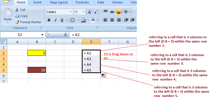
If you refer to cell B1 from cell E1, actually you would be referring to a cell that is 3 columns to the left (E-B = 3) within the same row number 1.
When it is copied to other locations present in a worksheet, the relative reference for that location will be changed automatically. (because relative cell reference describes offset to another cell rather than a fixed address as In our example, offset is : 3 columns left in the same row).
#Example 2:
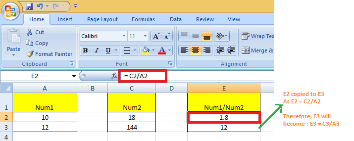
If you copy the formula = C2 / A2 from the cell “E2” to “E3”, the formula in E3 will automatically become =C3/A3.
When to Use Relative Cell References in Excel
When you need to develop a formula for a set of cells and the formula needs to make a reference to a relative cell reference, relative cell references come in handy.
When this occurs, you can create the formula in one cell and copy it before pasting it into every other cell.
2. Absolute Cell Reference
When copying or using AutoFill, there are times when the cell reference must stay the same. A column and/or row reference is kept constant using dollar signs. So, to get an absolute reference from a relative, we can use the dollar sign ($) characters.
To refer to an actual fixed location on a worksheet whenever copying is done, we use absolute reference. The reference here is locked such that rows and columns do not shift when copied.
How to Use Absolute Cell References in Excel
Below is an example depicting how to use Absolute Cell References in Excel.
#Example:
When we fix both row & column – Say if we want to lock row 2 & column A, we will use $A$2 as:
G2 = C2/$A$2, when copied to G3, G3 becomes = C3/$A$2
Note: C3 is 4 columns left to G3 in the same row.
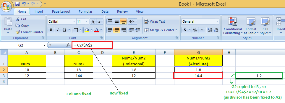
Here, original cell reference A2 is maintained whenever we copy G2 to any of the cells. So I3 = E3/$A$2 because E3 comes from the relative reference (4 columns left to the current one) & /$A$2 comes from the absolute reference.
Therefore, I3 = E3//$A$2 = 12/10 = 1.2
What Does the Dollar ($) Sign Do?
When the row and column numbers are preceded by the dollar symbol ($), it becomes absolute (i.e., stops the row and column number from changing when copied to other cells). Dollar ($) before the row fixes the row & before the column fixes the column.
When to Use Absolute Cell References in Excel
When you don’t want the cell reference to alter when you replicate formulas, absolute cell references come in handy. This can be the situation if you have to use a fixed value in the formula.
3. Mixed Cell Reference
An absolute column and relative row, or an absolute row and relative column, is a mixed cell reference. You get an absolute column or absolute row when you individually put the $ before the column letter or before the row number. Example: $B8 is relative to row 8 but absolute for column B, and B$8 is absolute for row 1 but relative for column A.
Here, the Dollar ($) before the row number fixes/locks the row & before the column name fixes/locks the column.
#Example:
When we fix the only row: If we have G2 = C2/A$2 then :
We used $ before the row number, so we are locking the only row here. When G2 is copied to G3, G3 = C3/A$2 (not C3/A3) because the row has been fixed already.
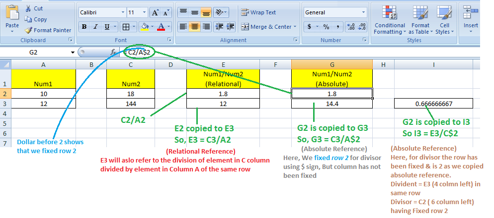
Here, whenever we copy G2 to any other cell, always the divisor will refer to a fixed row 2 (column vary according to the concept of relative reference)
So, when G2 is copied to I3, I3 = E3/C$2 because E3 comes from the relative reference (4 columns left to the current one) & C$2 comes from the absolute reference for row & relative reference for Column (6 Columns left to the current one)
Some Other Ways of Using Cell References With Examples
Now that we are familiar with the basics of using Cell References in Excel, let’s see some other ways of using cell references.
Relative and Absolute Cell References for Calculating Dates
We can use relative and absolute cell references to calculate dates.
Example: To Calculate the Date of Delivery online from the given date of the order placed & no of days it will take to deliver :
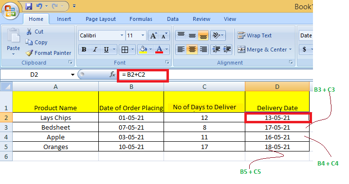
Here, We calculate the Date of Delivery by = Order Date + No of days to deliver. We used Relative cell reference so that individual product delivery dates can be calculated.
Absolute cell references for calculating dates :
Example: To Calculate the Date of Birth When the age is known is a number of days using Current date can be done by making use of absolute reference.
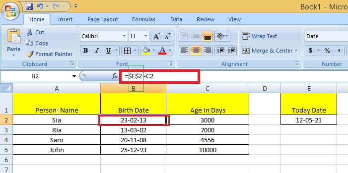
Here, We calculate DOB by = Current Date – Age in days. The Current date is contained in the cell E2 & in subtraction, we fixed that date to subtract from the days.
Whole Column Reference
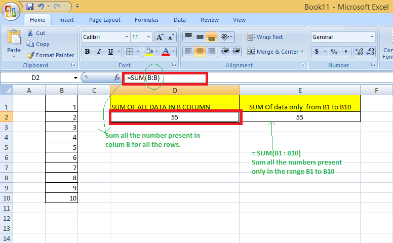
You will want to refer to all the cells inside a particular column when operating with an Excel worksheet with any number of rows. Simply type a column letter twice with a colon in between to refer to the entire column B, for example, B:B.
Example: You may want to find the sum of a column of data in certain cases. While you can do this with a regular cell range, such as =SUM(B1:B10), you will need to change the cell range if your spreadsheet grows in size.
Excel, on the other hand, has a cell range that does not require the row number and takes all the cells in the column in action. If you wanted to find the sum of all the values in column B, for example, you would type =SUM (B:B). You can add as much data as you want to your spreadsheet without having to change your cell ranges if you use this type of cell range.
Whole Row Reference
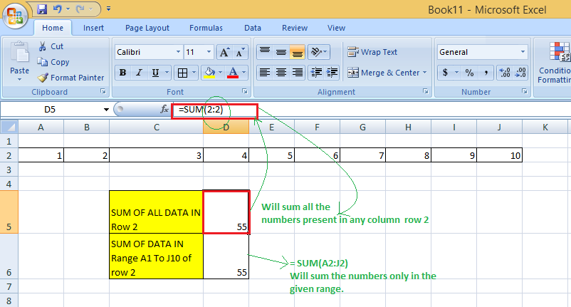
You will want to refer to all the cells inside a particular row when operating with an Excel worksheet with any number of columns. Simply type a row number twice with a colon in between to refer to the entire row, for example, 2:2.
Example: You may want to find the sum of a row of data in certain cases. While you can do this with a regular cell range, such as =SUM(A2 : J2), you will need to change the cell range if your spreadsheet grows in size.
Excel, on the other hand, has a cell range that does not require the column letter and takes all the cells in the row in action. If you wanted to find the sum of all the values in row 2, for example, you would type =SUM (2:2). You can add as much data as you want to your spreadsheet without having to change your cell ranges if you use this type of cell range.
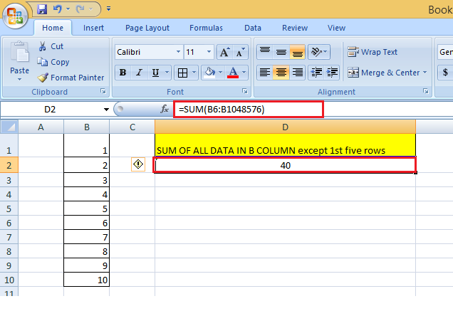
Refer to an Entire Column, Excluding the First Few Rows
To refer to the entire column excluding the first few rows, you need to specify the range as we give in a normal fashion. We know that the Excel worksheets can have only 1,048,576 rows. (To check this, go to an empty cell & press: Ctrl + Down arrow Key)
So, we can do the sum of the entire column B except for the first 5 rows by = SUM(B6:B1048576).
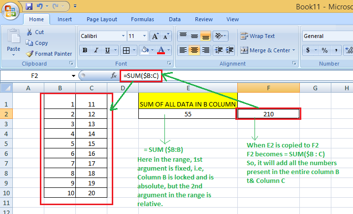
Using a Mixed Entire Column Reference in Excel
You can also create a mixed entire-column reference, say for example $B:B. But, practically, it is difficult to find a situation where it would be used.
Example :
How to switch between Absolute, Relative, and Mixed References
The $ sign can be manually typed in an Excel formula to adjust a relative cell relation to absolute or mixed. You can also speed things up by pressing the F4 key. You must be in formula edit mode to use the F4 shortcut. The steps are :
Firstly, choose the cell that contains the formula. Then, by pressing the F2 key or double-clicking the cell, you can enter Edit mode. Select the cell reference in which you want to make changes. Then, switch between four-cell reference forms by pressing F4.
Example: When you select a cell having only relative reference (i.e., no $ sign), say = B2:
- The first time when you press F4, it becomes =$B$2
- The second time when you press F4, it becomes =B$2
- The third time when you press F4, it becomes=$B2
- The fourth time when you press F4, it becomes back to the relative reference=B2
B2 –Press F4–> =$B$2 –Press F4–> =B$2 –Press F4–> = =$B2 –Press F4–> =B2
So, using F4, you do not require to manually type the $ symbol.
Important Points to Remember
- One of the crucial components for Excel functions or formulas is the cell reference.
- Excel formulas that employ relative cell references automatically change the references to match the correct row and column.
- When copying formulas into non-relative cells, absolute cell references are advised. Excel keeps the absolute cell references constant.
- According to the specifications, a mixed reference only locks one of the references, either the row or the column. Not both are locked.
FAQs on Excel Cell References
1. What are the 3 types of cell references in Excel?
Ans: In Excel, we can use one of three types of cell references:
- Relative Cell References
- Absolute Cell References
- Mixed Cell References
Cell References in Excel: Relative, Absolute, and Mixed (2023)
Cell references often confuse Excel users no matter how simple they may sound.
Be it Cell A1 or Cell XFD1048576. How are these cell references made?🤔
The guide below will teach you this and much more. So jump right in.
And as you go, download our free sample workbook here to practice along the guide.
What are cell references in Excel
Cell references are like the name of cells. A cell reference is alphanumeric; it consists of an alphabet and a number. 🔠
Where do this alphabet and number come from? Here is what a worksheet in Excel looks like (A two-dimensional window with rows and columns).

Columns in Excel are denoted by alphabet. Whereas rows in Excel are denoted by numbers.
A cell is formed at the intersection of a row and a column. It is then named as a combination of that row and column.
For example, in the image below the highlighted cell forms at the intersection of Column B and Row 2.

The highlighted cell is referred to as Cell B2 (Column B and row 2).
Similarly, drag your worksheet to the end to see if even the last cell (Cell XFD1048576) is referred to the same way.

It is formed at the intersection of Column XFD and Row 1048576.
Pro Tip!
Did you know? There are a total of 16,384 columns in Excel. And the total number of rows in Excel is 1,048,576. 💯
How to use cell references (relative references)
Cell references make your Excel jobs unbelievably easy. You can use them everywhere and the best thing – as you move the formulas, the cell reference automatically adjusts.
See here.

The image shows the total marks for each subject in Row 2. The percentage marks acquired by a student in each of these subjects is in Row 3.
Let’s quickly find the marks scored in each subject.
Write the formula in Cell B4 as follows:
= B2 * B3

We are multiplying Cell B2 (Total marks) by Cell B3 (Percentage). Excel calculates the obtained marks in English.

Let’s calculate the same for the remaining subjects. But don’t waste time writing the respective formula for each subject.
Drag and drop the formula in Cell B4 to the remaining cells.

Excel calculates the obtained marks for all the remaining subjects.
But what has Excel done?
When formulas are moved across cells, Excel changes the relative cell references based on the relative rows/columns.
For example, the above formula when copied from Column B to C becomes:
= C2 * C3

Move it from Column C to Column D to see it changes as follows.
= D2 * D3

That way, you do not have to write formulas unique to each cell.
You can put together a single formula for one cell and copy/paste it to the others. Excel will automatically update the relative cell references. 💪
How to use absolute cell references
What if the above data changes as shown below?

The data remains the same. However, marks for each of the subjects are not mentioned now. Instead, we have the total marks in Cell F2 only.
To calculate the marks obtained in English, write the formula below.
= B2 * F2

B2 consists of the percentage marks obtained in English. At the same time, Cell F2 consists of the total marks for all the subjects.
Excel calculates the marks obtained in English as below.

Can we move the same formula (drag and drop it) for the remaining subjects?

The results are bizarre. What has Excel done?

The cell references were relative. As we moved it from one column to another, Excel changed the column reference from F2 to G2. G2 is an empty cell, so, Excel returns zero.
In such a case, we don’t want Excel to change the cell reference (F2) every time the formula is moved. We want to keep it constant.
However, we want the cell reference for percentages to change every time the formula is moved.
Write the formula as follows.
= B2 * $F$2

We have changed the relative reference of Cell F2 into an absolute reference of $F$2.
Unlike relative cell references, an absolute cell reference has a dollar symbol before the column and the row reference. Like $A$1.
However, the cell reference B2 is still the same. This is because we only want to fix the cell reference $F$2 but not B2.
Drag and move it across all the columns

Excel calculates the obtained marks for all the subjects.
This time Excel updated the formula for each next column by changing the cell reference of B2 but not F2.
For example, when moved to Column C, Excel changes the formula as below.

So, the formula changes from:
=INDEX(D:D,MATCH(G2,A:A,0))
To:
=INDEX(D:D,MATCH(1,A:A,0))
The “theory” behind this is not as simple as changing the lookup value.
Since you’re changing the formula from a normal one to an array formula, the structure of the formula changes a bit as well. By changing the lookup value to 1, you’re not actually telling the MATCH function to search for the number 1 in the lookup array (last name column).
Pro Tip!
To change any reference into an absolute cell reference, click on that cell reference in the formula bar and press the F4 key.
Mixed cell referencing in Excel
Who said a cell reference has to be a relative or an absolute one only? There can be mixed cell references too.
Pro Tip!
A mixed cell reference is where any one component of the cell reference (column reference or the row reference) is absolute, and the other is relative.
For example, $C3 (Absolute column reference and relative row reference). Or C$3 (Relative column reference and absolute row reference).
The absolute reference comes after a dollar sign. 💲
For example, the image below the number of units sold for January and February.

To calculate the sales for both months, let’s multiply these by the price.
- Write the formula as:
= B2 * D2

- Drag and drop the same formula to all the products to get the sales for January.

What about February?
- Copy-paste the same formula into the column for February sales.

This is what happens when you do so. As we move the formula one column ahead, Excel changes the column references from B2 and D2 to C2 and E2.

We want Excel to multiply the units sold of each product for each month with the price. This means we want to keep the column of prices (Column D) constant.
- To do so, convert it into a mixed reference as follows.
= C2 * $D2

We only added a dollar sign ($) before the column reference (D). There is no dollar sign ($) before the row reference (2).
This way each time this formula is moved, the column will remain the same (Column D), but the row number would accordingly change.
- Drag and drop the formula now to see the results.

Excel now keeps Column D constant. All other references change with the relative position of the row/column.
Cell references to other worksheets
Cell references are not limited to a single sheet only. You can also create a reference to a cell from another worksheet. 🙌
See here. We have the value for Apples in Sheet 2.

We need this sales value in Sheet 1.
- To create a direct reference to Sheet 2, activate a cell in Sheet 1 and write an equal sign (=).

- Now go to sheet 2 and click on the targeted value (sales value of Apples).

- Press Enter.
- In sheet 1, a reference is created to Cell A2 of Sheet 2.

That is how you can create references to other cells across different worksheets of a workbook.
That’s it – Now what?
Cell references are one of the building blocks of Excel. Unless you understand how cell references work, you can barely use Microsoft Excel.
👉 The above guide teaches you how cell references are formed. We learned about all three types of cell references (mixed, relative, and absolute references). And also how they can be used within a worksheet and across worksheets.
To make your Excel jobs even simpler, you must master the SUMIF, IF, and VLOOKUP functions of Excel.
Click here to sign up for my 30-minute free email course that teaches you these and other functions of Excel.
Other resources
If you enjoyed learning about cell references, we bet you’d love to know more.
Just like cell references, there’s so much more to the basics of Excel that will change the way you work. Hop on here to learn how to select multiple cells and merge/unmerge cells in Excel.
Kasper Langmann2023-01-19T12:13:01+00:00
Page load link
,
What Do You Mean By Cell Reference in Excel?
A cell reference in Excel refers to other cells to a cell to use its values or properties. So in simple terms, if we have data in some random cell A2 and we want to use that value of cell A2 in cell A1, we can use =A2 in cell A1. So it will copy the value of A2 in A1. So it is called cell referencing in Excel.
For example, suppose you insert C1O. As a result, it will expand “Column C” and the “10th Row.” Likewise, we can also define or declare cell references to any location in the worksheet. We may also activate another way for cell reference, e.g., R7C7 from Excel “Options,” where R7 is Row 7 and C7 is Column 7.
Table of contents
- What Do You Mean By Cell Reference in Excel?
- Explained
- Types of Cell Reference in Excel
- #1 How to Use Relative Cell Reference?
- #2 How to Use Absolute Cell Reference?
- #3 How to Use Mixed Cell Reference?
- Things to Remember
- Recommended Articles
Explained
- Excel worksheet is made up of cells. Each cell has a cell reference.
- Cell reference contains one or more letters or the alphabet followed by a number where the letter or alphabet indicates the column and the number represents the row.
- Each cell can be located or identified by its cell reference or address, e.g., B5.
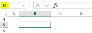
- Each cell in an Excel worksheet has a unique address. The address of each cell is defined by its location on the grid. g. In the below-mentioned screenshot, the address “B5” refers to the cell in the fifth row of column B.
Even if we enter the cell address directly in the grid or name window, it will go to that cell location in the worksheet. Cell references can refer to either one cell, a range of cells, or entire rows and columns.
When a cell reference refers to more than one cell, it is called “range.” E.g., A1:A8 indicates the first 8 cells in column A. In between, a colon is used.
Types of Cell Reference in Excel
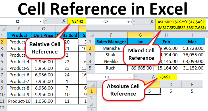
- Relative cell references: It does not contain dollar signs in a row or column, e.g., A2. Relative cell reference type in ExcelIn Excel, relative references are a type of cell reference that changes when the same formula is copied to different cells or worksheets. Let’s say we have =B1+C1 in cell A1, and we copy this formula to cell B2 and it becomes C2+D2.read more changes when a formula is copied or dragged to another cell. In Excel, cell referencing is relative by default. It is the most commonly used cell reference in the formula.
- Absolute cell references: Absolute cell reference Absolute reference in excel is a type of cell reference in which the cells being referred to do not change, as they did in relative reference. By pressing f4, we can create a formula for absolute referencing.read more contains dollar signs attached to each letter or number in a reference, e.g., $B$4. Suppose we mention a dollar sign before the column and row identifiers. It makes absolute or locks both the column and the row, i.e., where cell reference remains constant even if it is copied or dragged to another cell.
- Mixed cell references in Excel: In Excel, mixed cell references contain dollar signs attached to either the letter or the number in a reference. E.g., $B2 or B$4. It is a combination of relative and absolute references.
Now, let us discuss each cell reference in detail –
You can download this Cell Reference Excel Template here – Cell Reference Excel Template
#1 How to Use Relative Cell Reference?
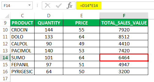
The below-mentioned pharma sales table below contains medicine “Products” in column C (C10:C16), “Quantity Sold” in column D (D10:D16), and “Total_Sales_Value” in column F, which we need to find out.
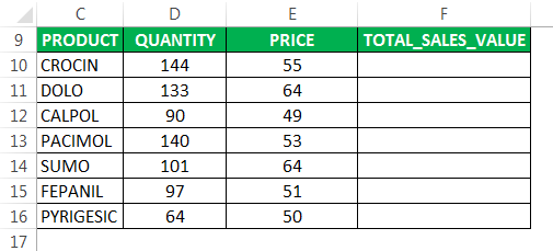
To calculate the total sales for each item, we need to multiply the price of each item by its quantity of that.
Let us check out the first item; for the first item, the formula in cell F10 would be multiplication in ExcelMultiplication in excel is performed by entering the comparison operator “equal to” (=), followed by the first number, the “asterisk” (*), and the second number.read more – D10*E10.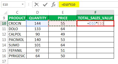
It returns the total sales value.

Instead of entering the formula for all the cells, we can apply a formula to the entire range. To copy the formula down the column, click inside cell F10 to see that the cell is selected. Then, select the cells till F16. So, that column range will get selected. Then, we will click “Ctrl+D” to apply the formula to the entire range.
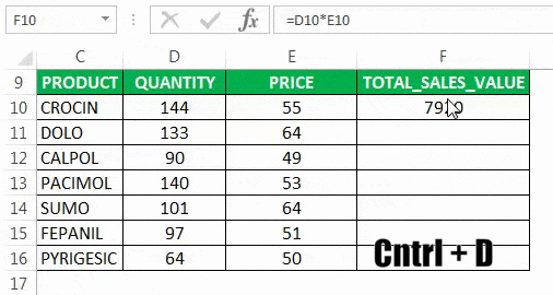
Here, when you copy or move a formula with a relative cell reference to another row. Automatically, row references will change (similarly for columns also)
We can notice that the cell reference automatically adjusts to the corresponding row.
To check a relative reference, we must select any of the “Total _Sales_ Value” cells in column F, and we can view the formula in the formula bar. E.g., In cell F14, we can observe that the formula has been changed from D10*E10 to D14*E14.
#2 How to Use Absolute Cell Reference?
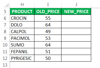
The below-mentioned pharma product table contains medicine “Products” in column H (H6:H12), and it’s “Old_Price” in column I (I6:I12), and “New_Price” in column J, which we need to find out with the help of absolute cell reference.
We can see that the rate for each product is increased by 5% effective from Jan 2019 and is listed in cell “K3”.
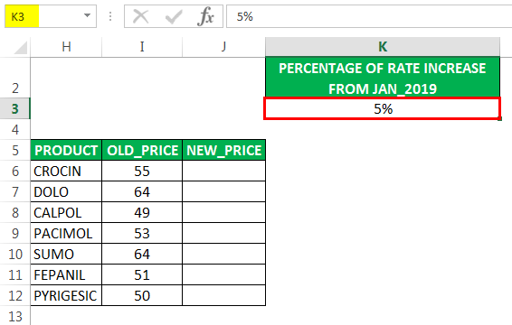
To calculate the “New_Price” for each item, we need to multiply the old price of each item by the percentage price increase (5%) and add the “Old_Price” to it.
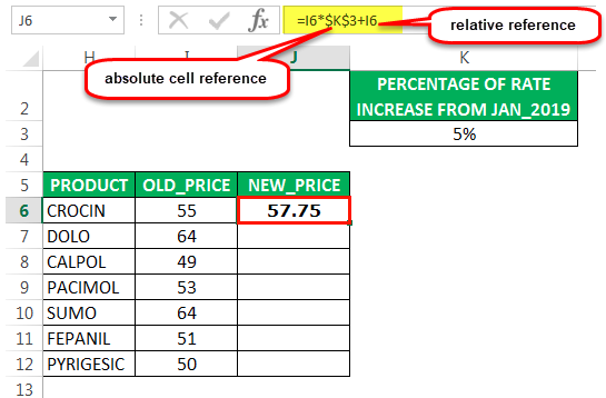
Let us check out the first item. For the first item, the formula in cell J6 would be =I6*$K$3+I6, which returns the new price.
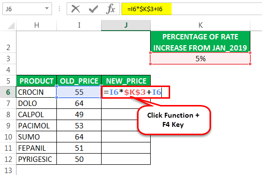
Here, the percentage rate increase for each product is 5%, a common factor. Therefore, we must add a dollar symbol in front of the row and column number for the cell “K3” to make it an absolute reference, i.e., $K$3. We can add it by clicking the “function+F4” key once.
Here the dollar sign for the cell “K3” fixes the reference to a given cell, where it remains unchanged no matter when you copy or apply a formula to other cells.
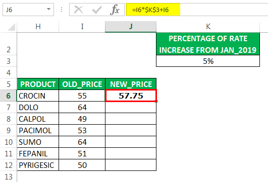
Here, $K$3 is an absolute cell reference, whereas “I6” is a relative cell reference. It changes when you apply it to the next cell.
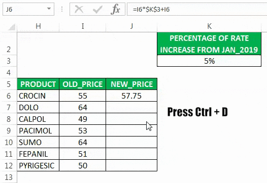
Instead of entering the formula for all the cells, we can apply a formula to the entire range. To copy the formula down the column, click inside cell J6 to see that the cell has been selected. Then, we must select the cells till J12. So, that column range will get selected. Then click “Ctrl+D” so the formula is applied to the entire range.
#3 How to Use Mixed Cell Reference?
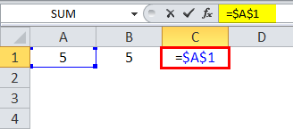
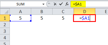
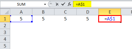
In the below-mentioned table, we have values in each row (D22, D23, and D24) and columns (E21, F21, and G21). Here, we have to multiply each column with each row with the help of a mixed cell reference.
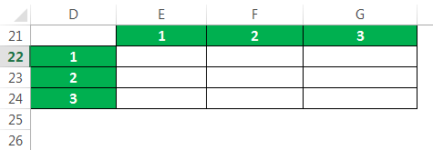
We can use two mixed-cell references here to get the desired output.
Let us apply two types of mixed references below in cell “E22.”
The formula would be =$D22*E$21

#1 – $D22: Absolute column and Relative row

The dollar sign before column D indicates that only the row number can change. At the same time, the column letter D is fixed. It does not change.
When we copy the formula to the right side, the reference will not change because it is locked, but When you copy it down, the row number will change because it is not locked.
#2 – E$21: Absolute row and Relative column
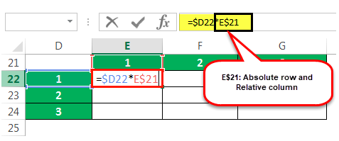
The dollar sign right before the row number indicates only the column letter E can change. Whereas the row number is fixed; it does not change.
The row number will not change when copying the formula because it is locked. But when we copy the formula to the right side, the column alphabet will change because it is not locked.
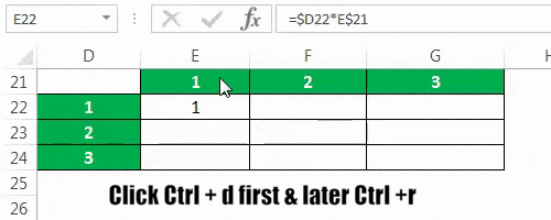
Instead of entering the formula for all the cells, we can apply a formula to the entire range. Now, we will click inside cell E22. As a result, first, we will see that the cell is selected. Then, we will select the cells until G24 so that the entire range will get selected. Next, we will click on the “Ctrl+D” key and, later, “Ctrl+R.”
Things to Remember
- The cell reference is a key element of formula or excels functions.
- Cell references are used in Excel functions, formulas, charts, and various other Excel commandsVLOOKUP function, IF condition, CONCATENATE function, find MAXIMUM and MINIMUM values are the most commonly used excel commands.read more.
- Mixed reference locks either of one. It may be a row or column, but not both.
Recommended Articles
This article is a guide to Cell Reference in Excel. We discuss how to cell references in Excel, along with three types, examples, and downloadable templates. You may learn more about Excel from the following articles: –
- 3D Reference Excel – Examples
- Timesheet in Excel
- Excel Auto Numbering
- Solver in Excel
- Programming in Excel
Excel Cell Reference (Table of Contents)
- Cell Reference in Excel
- Types of Cell Reference in Excel
- #1 – Relative Cell Reference in Excel
- #2- Absolute Cell Reference in Excel
- #3- Mixed Cell Reference in Excel
Cell Reference in Excel
Cell Reference in excel is the way to represent the identity and the location of any cell with the help of combining Column Name and Row Number on a worksheet. For example, if we say cell B10, then it expands as Column B and 10th Row. Similarly, we can define or declare cell references to any position in the worksheet. We can also activate R1C1 from Excel Options, another way for cell reference, where R1 is Row1 and C1 is Column1.
Types of Cell Reference in Excel
We have three different types of Cell References in Excel –
- Relative Cell Reference in Excel
- Absolute Cell Reference in Excel
- Mixed Cell Reference in Excel
Using the correct type of Cell Reference in a particular scenario will save a lot of time and effort and make the work much easier.
#1 – Relative Cell Reference in Excel
Relative cell references in excel refer to a cell or a range of cells in excel. Every time a value is entered into a formula, such as SUMIFS, it is possible to input into Excel a “cell reference” as a substitute for a hard-coded number. A cell reference may come in the form B2, where B corresponds to the cell column letter in question and 2 represents the row number. Whenever Excel comes across a cell reference, it visits the particular cell, extracts out its value, and uses that value in whichever formula that you’re writing. When this cell reference in excel is duplicated to a different location, the relative cell references in excel correspondingly also change automatically.
When we refer to cells like this, we can achieve it with any of the two cell reference types in excel: absolute and relative. The demarcation between these two distinct reference types is the different inherent behavior when you drag or copy and paste them to different cells. Relative Cell references can alter themselves and adjust as you copy and paste them; absolute references contrarily do not. Therefore, in order to successfully achieve results in Excel, it is critical to be able to use relative and absolute cell references in the right way.
How to effectively use Relative cell reference in Excel?
To comprehensively understand the versatility and usability of this amazing feature of Excel, we will need to look at a few practical examples to grasp its true value.
You can download this Cell Reference Excel Template here – Cell Reference Excel Template
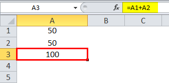
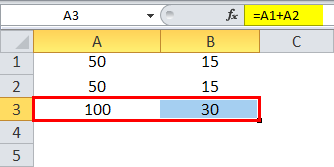
Example #1
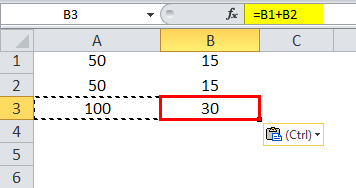
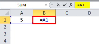
Let us consider a simple example to explain the mechanics of Relative Cell Reference in Excel. If we wish to have the sum of two numbers in two different cells – A1 and A2, and have the result in a third cell A3.
So we apply the formula =A1+A2
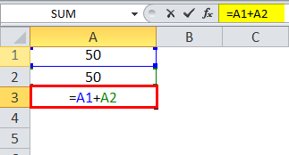
Which would yield the result as 100 in A3.
Now suppose, we have a similar scenario in the next column (B). Cell B1 and B2 have two numbers, and we wish to have the sum in B3.
We can achieve this in two different ways:
Here we physically write the formula to add the two cells B1 and B2 in B3.
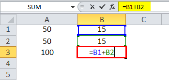
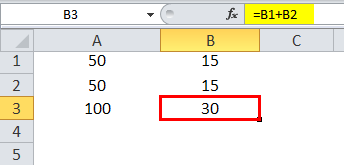
The result is 30.
Or we could simply copy the formula from cell A3 and paste it into cell B3 (it would work if we drag the formula from A3 to B3 also).
So, when we copy the contents of cell A3 and paste in B3 or drag the contents of cell A3 and paste in B3, the formula gets copied, not the result. We could achieve the same result by right-clicking on cell A3 and use the Copy option.
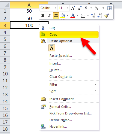
And after that, we move to the next cell, B3, and right-click and select “Formulas (f)”.
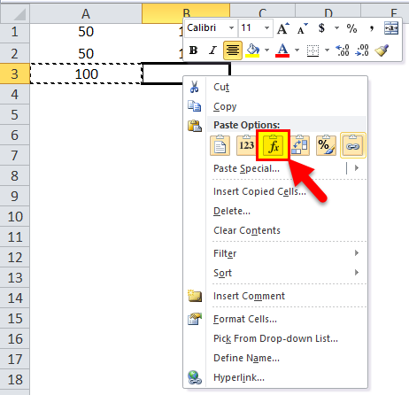
What this means is that cell A3=A1+A2. When we copy A3 and move one cell to the right and paste it onto cell B3, the formula automatically adapts itself and changes to become B3=B1+B2. It applies the summation formula for B1 and B2 cells instead.
Example #2
Now, let’s look at yet another practical scenario that would make the concept quite clear. Let us assume that we have a data set consisting of the Unit Price of a product and the quantity sold for each of them. Now our objective is to calculate the Sale Price, which the following formula can describe:
Sale Price = Unit Price x Units Sold.
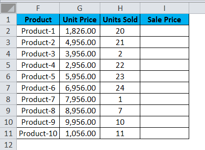
To be able to find the Sale Price, we need to now multiply Unit Price with Units Sold for each product. So, we shall now proceed to apply this formula for the first cell in Sale Price, i.e. for Product 1.
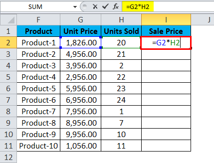
When we apply the formula, we get the following result for Product 1:
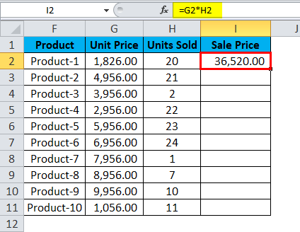
It successfully multiplied the Unit Cost by the Units Sold for Product 1, i.e. cell G2 * cell H2, i.e. 1826.00 * 20, which gives us the result 36520.00.
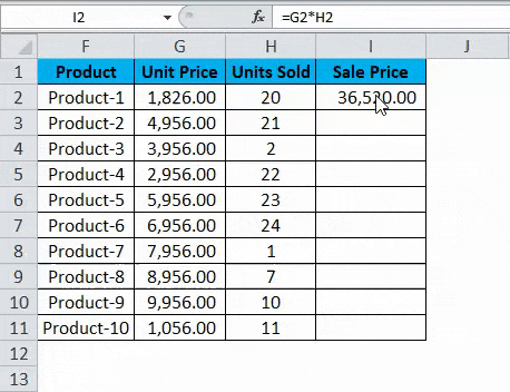
So now we see that we have 9 other products to go. In real case scenarios, this could go up to hundreds or thousands of rows. It becomes difficult and nearly impossible to simply go about writing the formula for each row.
Hence, we will use the Relative Reference feature of Excel and simply copy the contents of cell I2 and paste in all of the remaining cells in the table for the column Sale Price or simply drag the formula from cell I2 to the rest of the rows in that column and get the results for the whole table in less than 5 seconds.
Here we press Ctrl + D. So the output will look like below:
#2 – Absolute Cell Reference in Excel
Most of our daily work in Excel involves handling formulae. Therefore, having a working knowledge of Relative, Absolute, or Mixed cell References in excel becomes quite important.
Let us see the following:
=A1 is a relative reference, where both the row and column change when we copy the formula cell.
=$A$1 is an absolute cell reference; both the column and row are locked and do not change when we copy the formula cell. Thus, the cell value remains constant.
In =$A1, the column is locked, and the row can keep changing for that specific column.
In =A$1, the row is locked, and the column can keep changing for that specific row.
Unlike Relative Reference, which can change as it moves to different cells, the absolute reference doesn’t change. The only thing required here is to lock the specific cell completely.
Using a dollar sign in the formula, w.r.t. a cell reference makes it an absolute cell reference as the dollar sign locks the cell. We can lock either the row or the column using the dollar sign. If the “$” is before an alphabet, then it locks a column, and if the “$” is before a number, then a row is locked.
#3- Mixed Cell Reference in Excel
How to effectively use Absolute cell reference in Excel also how to use Mixed cell Reference in excel?
To get a comprehensive understanding of Absolute and Mixed cell Reference in excel, let us look at the following example.
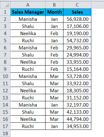
We have the sales data for 4 sales managers across different months, where sales have occurred multiple times in a month.
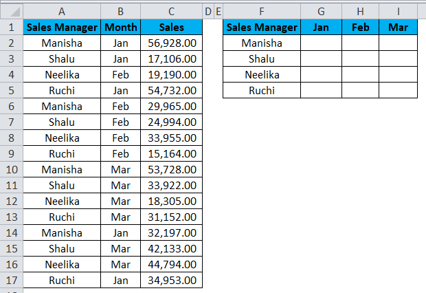
Our objective is to calculate the consolidated sales summary of all 4 sales managers. We shall apply the SUMIFS formula to get the desired result.
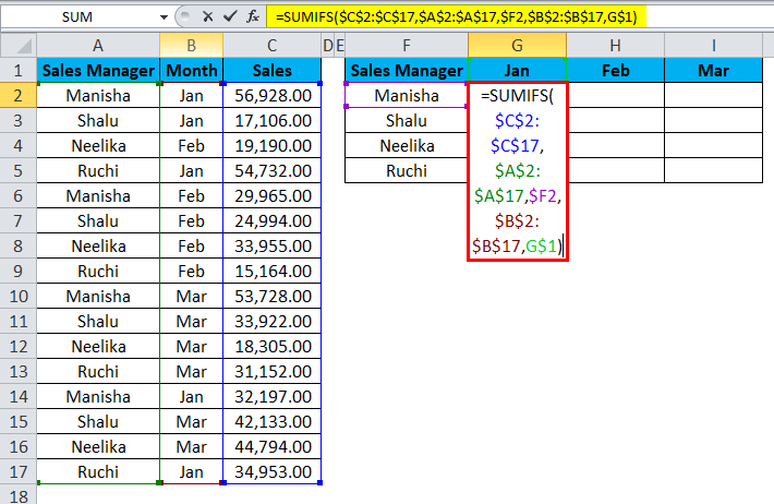
The result will be as:
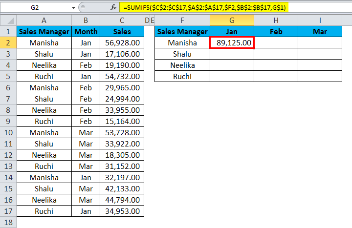
Let us observe the formula to see what happened.
- In the “sum_range”, we have $C$2:$C$17. There is a dollar sign in front of both the alphabet and the numbers. Thus, both the rows and columns for the cell range are locked. This is an absolute cell reference.
- Next, we have “criteria_range1”. Here too, we have absolute cell reference.
- After this, we have “criteria1” – $F2. Here we see that only the column will be locked while copying the formula cell, meaning only the row will change when we copy the formula to a different cell (moving down). This is a mixed cell reference.
- Next, we have “criteria_range2”, which is also an absolute cell reference.
- The final segment of the formula is “criteria2” – G$1. Here we observe that the dollar sign is present in front of the number and not the alphabet. Thus, only the row is locked when we copy the formula cell. The column can change when we copy the formula cell to a different cell (moving right). This is a mixed cell reference.
Dragging the formula across the summary table by pressing the Ctrl+D key first and later Ctrl+R. We get the following result:
Mixed cell reference refers to a particular row or column only, such as =$A2 or =A$2. If we want to create a mixed cell reference, we can press the F4 key on the formula two to three times, as per your requirement, i.e. to refer to a row or a column. Pressing F4 again will cause the cell reference to change to relative reference.
Things to Remember
- While copying the Excel formula, relative referencing is generally what is desired. This is the reason why this is the default behavior of Excel. But sometimes, the objective might be to apply absolute reference rather than relative Cell reference in excel. Absolute Reference is making a cell reference fixed to an absolute cell address, due to which, when the formula is copied, it remains unaltered.
- Absolutely no dollar signs are required with Relative referencing. When we copy the formula from one place to others, the formula will adapt accordingly. So, if we type =B1+B2 into cell B3 and then drag or copy-paste the same formula into the cell C3, the Relative Cell reference would automatically adjust the formula to =C1+C2.
- With Relative referencing, the referred cells automatically adjust themselves in the formula as per your movement, either to the right, left, upward or downwards.
- With Relative referencing, if we were to give a reference to cell D10 and then shift one cell downwards, it would change to D11; if instead, we shift one cell upwards, it would change to D9. If we shift one cell to the right, the reference will change to E10, and instead, if we shift one cell to the left, the reference would automatically adjust itself to C10.
- Pressing F4 once will change relative Cell reference to absolute Cell reference in excel.
- Pressing F4 twice will change the cell reference to a mixed reference where the row is locked.
- Pressing F4 thrice will change the cell reference to a mixed reference where the column is locked.
- Pressing F4 for the fourth time will change the cell reference back to the relative reference in excel.
Recommended Articles
This has been a guide to Cell Reference in Excel. Here we discuss three types of cell reference in excel, i.e. absolute, relative, and mixed cell reference, and how to use each of them along with practical examples and a downloadable excel template. You can also go through our other suggested articles –
- Relative Reference in Excel
- New Line in Excel Cell
- SUM Cells in Excel
- Divide Cell in Excel