Cell offset excel vba - Word и Excel - помощь в работе с программами

Return to VBA Code Examples

The Offset Property is used to return a cell or a range, that is relative to a specified input cell or range.

Using Offset with the Range Object

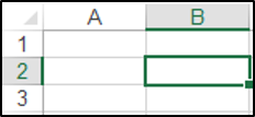
You could use the following code with the Range object and the Offset property to select cell B2, if cell A1 is the input range:

Range("A1").Offset(1, 1).Select

The result is:

Notice the syntax:

Range.Offset(RowOffset, ColumnOffset)

Positive integers tells Offset to move down and to the right. Negative integers move up and to the left.

The Offset property always starts counting from the top left cell of the input cell or range.

Using Offset with the Cells Object

You could use the following code with the Cells object and the Offset property to select cell C3 if cell D4 is the input range:

Cells(4, 4).Offset(-1, -1).Select

Selecting a Group of Cells

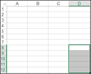
You can also select a group of cells using the Offset property. The following code will select the range which is 7 rows below and 3 columns to the right of input Range(“A1:A5”):

Range("A1:A5").Offset(7, 3).Select

Range(“D8:D12”) is selected:

VBA Coding Made Easy

Stop searching for VBA code online. Learn more about AutoMacro — A VBA Code Builder that allows beginners to code procedures from scratch with minimal coding knowledge and with many time-saving features for all users!

Learn More!

Источник

Свойство Offset объекта Range, возвращающее смещенный диапазон, в том числе отдельную ячейку, в коде VBA Excel. Синтаксис, параметры, примеры.

Offset – это свойство объекта Range, возвращающее диапазон той же размерности, но смещенный относительно указанного диапазона на заданное количество строк и столбцов.

Синтаксис

Синтаксис свойства Range.Offset:

Expression.Offset (RowOffset, ColumnOffset)

Expression – это выражение (переменная), возвращающее исходный объект Range, относительно которого производится смещение.

Параметры

RowOffset – это параметр, задающий смещение диапазона по вертикали относительно исходного на указанное количество строк.

Значение RowOffset	Направление смещения
Отрицательное	вверх
Положительное	вниз
0 (по умолчанию)	нет смещения

ColumnOffset – это параметр, задающий смещение диапазона по горизонтали относительно исходного на указанное число столбцов.

Значение ColumnOffset	Направление смещения
Отрицательное	влево
Положительное	вправо
0 (по умолчанию)	нет смещения

Необходимо следить за тем, чтобы возвращаемый диапазон не вышел за пределы рабочего листа Excel. В противном случае VBA сгенерирует ошибку (Пример 3).

Примеры

Пример 1
Обращение к ячейкам, смещенным относительно ячейки A1:

Sub Primer1()

Cells(1, 1).Offset(5).Select

MsgBox ActiveCell.Address

Cells(1, 1).Offset(, 2).Select

MsgBox ActiveCell.Address

Cells(1, 1).Offset(5, 2).Select

MsgBox ActiveCell.Address

End Sub

Пример 2
Обращение к диапазону, смещенному относительно исходного:

Sub Primer2()

Range(«C8:F12»).Offset(—3, 5).Select

MsgBox Selection.Address

End Sub

Пример 3
Пример ошибки при выходе за границы диапазона рабочего листа:

Sub Primer3()

On Error GoTo ErrorText

Cells(1, 1).Offset(—3).Select

Exit Sub

ErrorText:

MsgBox «Ошибка: « & Err.Description

End Sub

Источник

Excel VBA OFFSET Function

VBA Offset function one may use to move or refer to a reference skipping a particular number of rows and columns. The arguments for this function in VBA are the same as those in the worksheet.

For example, assume you have a data set like the one below.

Now from cell A1, you want to move down four cells and select that 5th cell, the A5 cell.

Similarly, if you want to move two rows down from the A1 cell and two columns to the right, select that cell, i.e., the C2 cell.

In these cases, the OFFSET function is very helpful. Especially in VBA OFFSET, the function is just phenomenal.

Excel VBA OFFSET Function
- OFFSET is Used with Range Object in Excel VBA
- Syntax of OFFSET in VBA Excel
- Examples
  - Example #1
  - Example #2
  - Example #3
  - Example #4
- Things to Remember
- Recommended Articles

OFFSET is Used with Range Object in Excel VBA

In VBA, we cannot directly enter the word OFFSET. Instead, we need to use the VBA RANGE objectRange is a property in VBA that helps specify a particular cell, a range of cells, a row, a column, or a three-dimensional range. In the context of the Excel worksheet, the VBA range object includes a single cell or multiple cells spread across various rows and columns.read more first. Then, from that range object, we can use the OFFSET property.

In Excel, the range is nothing but a cell or range of the cell. Since OFFSET refers to cells, we need to use the object RANGE first, and then we can use the OFFSET method.

Syntax of OFFSET in VBA Excel

Row Offset: How many rows do you want to offset from the selected cell? Here the selected cell is A1, i.e., Range (“A1”).
Column Offset: How many columns do you want to offset from the selected cell? Here, the selected cell is A,1, i.e., Range (“A1”).

Examples

You can download this VBA OFFSET Template here – VBA OFFSET Template

Example #1

Consider the below data for demonstration.

Now, we want to select cell A6 from cell A1. But, first, start the macro and reference cell using the Range object.

Code:

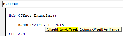
Sub Offset_Example1()

    Range("A1").offset(

End Sub

Now, we want to select cell A6. Then, we want to go down 5 cells. So, enter 5 as the parameter for Row Offset.

Code:

Sub Offset_Example1()

    Range("A1").offset(5

End Sub

Since we are selecting the same column, we leave out the column part. Close the bracket, put a dot (.), and type the method “Select.”

Code:

Sub Offset_Example1()

    Range("A1").Offset(5).Select

End Sub

Now, run this code using the F5 key, or you can run it manually to select cell A6, as shown below.

Output:

Example #2

Now, take the same data, but here will also see how to use the column offset argument. Now, we want to select cell C5.

Since we want to select cell C5 firstly, we want to move down four cells and take the right two columns to reach cell C5. The below code would do the job for us.

Code:

Sub Offset_Example2()

    Range("A1").Offset(4, 2).Select

End Sub

We run this code manually or using the F5 key. Then, it will select cell C5, as shown in the below screenshot.

Output:

Example #3

We have seen how to offset rows and columns. We can also select the above cells from the specified cells. For example, if you are in cell A10 and want to select the A1 cell, how do you select it?

In the case of moving down the cell, we can enter a positive number, so here in the case of moving up, we need to enter negative numbers.

From the A9 cell, we need to move up by 8 rows, i.e., -8.

Code:

Sub Offset_Example1()

    Range("A9").Offset(-8).Select

End Sub

If you run this code using the F5 key or manually run it, it will select cell A1 from the A9 cell.

Output:

Example #4

Assume you are in cell C8. From this cell, you want to select cell A10.

From the active cell, i.e., the C8 cell, we need to first move down 2 rows and move to the left by 2 columns to select cell A10.

In case of moving left to select the column, we need to specify the number is negative. So, here we need to come back by -2 columns.

Code:

Sub Offset_Example2()

    Range("C8").Offset(2, -2).Select

End Sub

Now, run this code using the F5 key or run it manually. It will select the A10 cell as shown below:

Output:

Things to Remember

In moving up rows, we need to specify the number in negatives.
In case of moving left to select the column, the number should be negative.
A1 cell is the first row and first column.
The “Active Cell” means presently selected cells.
To select the cell using OFFSET, you need to mention “.Select.”
To copy the cell using OFFSET, you need to mention “.Copy.”

A Quick Guide to Ranges and Cells

Function	Takes	Returns	Example	Gives
Range	cell address	multiple cells	.Range(«A1:A4»)	$A$1:$A$4
Cells	row, column	one cell	.Cells(1,5)	$E$1
Offset	row, column	multiple cells	Range(«A1:A2») .Offset(1,2)	$C$2:$C$3
Rows	row(s)	one or more rows	.Rows(4) .Rows(«2:4»)	$4:$4 $2:$4
Columns	column(s)	one or more columns	.Columns(4) .Columns(«B:D»)	$D:$D $B:$D

Download the Code

The Webinar

If you are a member of the VBA Vault, then click on the image below to access the webinar and the associated source code.

(Note: Website members have access to the full webinar archive.)

Introduction

This is the third post dealing with the three main elements of VBA. These three elements are the Workbooks, Worksheets and Ranges/Cells. Cells are by far the most important part of Excel. Almost everything you do in Excel starts and ends with Cells.

Generally speaking, you do three main things with Cells

Read from a cell.
Write to a cell.
Change the format of a cell.

Excel has a number of methods for accessing cells such as Range, Cells and Offset.These can cause confusion as they do similar things and can lead to confusion

In this post I will tackle each one, explain why you need it and when you should use it.

Let’s start with the simplest method of accessing cells – using the Range property of the worksheet.

Important Notes

I have recently updated this article so that is uses Value2.

You may be wondering what is the difference between Value, Value2 and the default:

' Value2
Range("A1").Value2 = 56

' Value
Range("A1").Value = 56

' Default uses value
Range("A1") = 56

Using Value may truncate number if the cell is formatted as currency. If you don’t use any property then the default is Value.

It is better to use Value2 as it will always return the actual cell value(see this article from Charle Williams.)

The Range Property

The worksheet has a Range property which you can use to access cells in VBA. The Range property takes the same argument that most Excel Worksheet functions take e.g. “A1”, “A3:C6” etc.

The following example shows you how to place a value in a cell using the Range property.

' https://excelmacromastery.com/
Public Sub WriteToCell()

    ' Write number to cell A1 in sheet1 of this workbook
    ThisWorkbook.Worksheets("Sheet1").Range("A1").Value2 = 67

    ' Write text to cell A2 in sheet1 of this workbook
    ThisWorkbook.Worksheets("Sheet1").Range("A2").Value2 = "John Smith"

    ' Write date to cell A3 in sheet1 of this workbook
    ThisWorkbook.Worksheets("Sheet1").Range("A3").Value2 = #11/21/2017#

End Sub

As you can see Range is a member of the worksheet which in turn is a member of the Workbook. This follows the same hierarchy as in Excel so should be easy to understand. To do something with Range you must first specify the workbook and worksheet it belongs to.

For the rest of this post I will use the code name to reference the worksheet.

The following code shows the above example using the code name of the worksheet i.e. Sheet1 instead of ThisWorkbook.Worksheets(“Sheet1”).

' https://excelmacromastery.com/
Public Sub UsingCodeName()

    ' Write number to cell A1 in sheet1 of this workbook
    Sheet1.Range("A1").Value2 = 67

    ' Write text to cell A2 in sheet1 of this workbook
    Sheet1.Range("A2").Value2 = "John Smith"

    ' Write date to cell A3 in sheet1 of this workbook
    Sheet1.Range("A3").Value2 = #11/21/2017#

End Sub

You can also write to multiple cells using the Range property

' https://excelmacromastery.com/
Public Sub WriteToMulti()

    ' Write number to a range of cells
    Sheet1.Range("A1:A10").Value2 = 67

    ' Write text to multiple ranges of cells
    Sheet1.Range("B2:B5,B7:B9").Value2 = "John Smith"

End Sub

You can download working examples of all the code from this post from the top of this article.

The Cells Property of the Worksheet

The worksheet object has another property called Cells which is very similar to range. There are two differences

Cells returns a range of one cell only.
Cells takes row and column as arguments.

The example below shows you how to write values to cells using both the Range and Cells property

' https://excelmacromastery.com/
Public Sub UsingCells()

    ' Write to A1
    Sheet1.Range("A1").Value2 = 10
    Sheet1.Cells(1, 1).Value2  = 10

    ' Write to A10
    Sheet1.Range("A10").Value2 = 10
    Sheet1.Cells(10, 1).Value2  = 10

    ' Write to E1
    Sheet1.Range("E1").Value2 = 10
    Sheet1.Cells(1, 5).Value2  = 10

End Sub

You may be wondering when you should use Cells and when you should use Range. Using Range is useful for accessing the same cells each time the Macro runs.

For example, if you were using a Macro to calculate a total and write it to cell A10 every time then Range would be suitable for this task.

Using the Cells property is useful if you are accessing a cell based on a number that may vary. It is easier to explain this with an example.

In the following code, we ask the user to specify the column number. Using Cells gives us the flexibility to use a variable number for the column.

' https://excelmacromastery.com/
Public Sub WriteToColumn()

    Dim UserCol As Integer
    
    ' Get the column number from the user
    UserCol = Application.InputBox(" Please enter the column...", Type:=1)
    
    ' Write text to user selected column
    Sheet1.Cells(1, UserCol).Value2 = "John Smith"

End Sub

In the above example, we are using a number for the column rather than a letter.

To use Range here would require us to convert these values to the letter/number cell reference e.g. “C1”. Using the Cells property allows us to provide a row and a column number to access a cell.

Sometimes you may want to return more than one cell using row and column numbers. The next section shows you how to do this.

Using Cells and Range together

As you have seen you can only access one cell using the Cells property. If you want to return a range of cells then you can use Cells with Ranges as follows

' https://excelmacromastery.com/
Public Sub UsingCellsWithRange()

    With Sheet1
        ' Write 5 to Range A1:A10 using Cells property
        .Range(.Cells(1, 1), .Cells(10, 1)).Value2 = 5

        ' Format Range B1:Z1 to be bold
        .Range(.Cells(1, 2), .Cells(1, 26)).Font.Bold = True

    End With

End Sub

As you can see, you provide the start and end cell of the Range. Sometimes it can be tricky to see which range you are dealing with when the value are all numbers. Range has a property called Address which displays the letter/ number cell reference of any range. This can come in very handy when you are debugging or writing code for the first time.

In the following example we print out the address of the ranges we are using:

' https://excelmacromastery.com/
Public Sub ShowRangeAddress()

    ' Note: Using underscore allows you to split up lines of code
    With Sheet1

        ' Write 5 to Range A1:A10 using Cells property
        .Range(.Cells(1, 1), .Cells(10, 1)).Value2 = 5
        Debug.Print "First address is : " _
            + .Range(.Cells(1, 1), .Cells(10, 1)).Address

        ' Format Range B1:Z1 to be bold
        .Range(.Cells(1, 2), .Cells(1, 26)).Font.Bold = True
        Debug.Print "Second address is : " _
            + .Range(.Cells(1, 2), .Cells(1, 26)).Address

    End With

End Sub

In the example I used Debug.Print to print to the Immediate Window. To view this window select View->Immediate Window(or Ctrl G)

You can download all the code for this post from the top of this article.

The Offset Property of Range

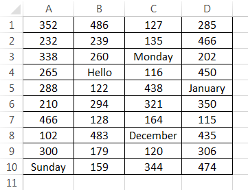
Range has a property called Offset. The term Offset refers to a count from the original position. It is used a lot in certain areas of programming. With the Offset property you can get a Range of cells the same size and a certain distance from the current range. The reason this is useful is that sometimes you may want to select a Range based on a certain condition. For example in the screenshot below there is a column for each day of the week. Given the day number(i.e. Monday=1, Tuesday=2 etc.) we need to write the value to the correct column.

We will first attempt to do this without using Offset.

' https://excelmacromastery.com/
' This sub tests with different values
Public Sub TestSelect()

    ' Monday
    SetValueSelect 1, 111.21
    ' Wednesday
    SetValueSelect 3, 456.99
    ' Friday
    SetValueSelect 5, 432.25
    ' Sunday
    SetValueSelect 7, 710.17

End Sub

' Writes the value to a column based on the day
Public Sub SetValueSelect(lDay As Long, lValue As Currency)

    Select Case lDay
        Case 1: Sheet1.Range("H3").Value2 = lValue
        Case 2: Sheet1.Range("I3").Value2 = lValue
        Case 3: Sheet1.Range("J3").Value2 = lValue
        Case 4: Sheet1.Range("K3").Value2 = lValue
        Case 5: Sheet1.Range("L3").Value2 = lValue
        Case 6: Sheet1.Range("M3").Value2 = lValue
        Case 7: Sheet1.Range("N3").Value2 = lValue
    End Select

End Sub

As you can see in the example, we need to add a line for each possible option. This is not an ideal situation. Using the Offset Property provides a much cleaner solution

' https://excelmacromastery.com/
' This sub tests with different values
Public Sub TestOffset()

    DayOffSet 1, 111.01
    DayOffSet 3, 456.99
    DayOffSet 5, 432.25
    DayOffSet 7, 710.17

End Sub

Public Sub DayOffSet(lDay As Long, lValue As Currency)

    ' We use the day value with offset specify the correct column
    Sheet1.Range("G3").Offset(, lDay).Value2 = lValue

End Sub

As you can see this solution is much better. If the number of days in increased then we do not need to add any more code. For Offset to be useful there needs to be some kind of relationship between the positions of the cells. If the Day columns in the above example were random then we could not use Offset. We would have to use the first solution.

One thing to keep in mind is that Offset retains the size of the range. So .Range(“A1:A3”).Offset(1,1) returns the range B2:B4. Below are some more examples of using Offset

' https://excelmacromastery.com/
Public Sub UsingOffset()

    ' Write to B2 - no offset
    Sheet1.Range("B2").Offset().Value2 = "Cell B2"

    ' Write to C2 - 1 column to the right
    Sheet1.Range("B2").Offset(, 1).Value2 = "Cell C2"

    ' Write to B3 - 1 row down
    Sheet1.Range("B2").Offset(1).Value2 = "Cell B3"

    ' Write to C3 - 1 column right and 1 row down
    Sheet1.Range("B2").Offset(1, 1).Value2 = "Cell C3"

    ' Write to A1 - 1 column left and 1 row up
    Sheet1.Range("B2").Offset(-1, -1).Value2 = "Cell A1"

    ' Write to range E3:G13 - 1 column right and 1 row down
    Sheet1.Range("D2:F12").Offset(1, 1).Value2 = "Cells E3:G13"

End Sub

Using the Range CurrentRegion

CurrentRegion returns a range of all the adjacent cells to the given range.

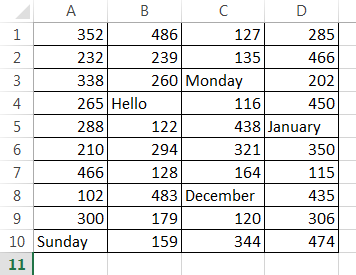
In the screenshot below you can see the two current regions. I have added borders to make the current regions clear.

A row or column of blank cells signifies the end of a current region.

You can manually check the CurrentRegion in Excel by selecting a range and pressing Ctrl + Shift + *.

If we take any range of cells within the border and apply CurrentRegion, we will get back the range of cells in the entire area.

For example
Range(“B3”).CurrentRegion will return the range B3:D14
Range(“D14”).CurrentRegion will return the range B3:D14
Range(“C8:C9”).CurrentRegion will return the range B3:D14
and so on

How to Use

We get the CurrentRegion as follows

' Current region will return B3:D14 from above example
Dim rg As Range
Set rg = Sheet1.Range("B3").CurrentRegion

Read Data Rows Only

Read through the range from the second row i.e.skipping the header row

' Current region will return B3:D14 from above example
Dim rg As Range
Set rg = Sheet1.Range("B3").CurrentRegion

' Start at row 2 - row after header
Dim i As Long
For i = 2 To rg.Rows.Count
    ' current row, column 1 of range
    Debug.Print rg.Cells(i, 1).Value2
Next i

Remove Header

Remove header row(i.e. first row) from the range. For example if range is A1:D4 this will return A2:D4

' Current region will return B3:D14 from above example
Dim rg As Range
Set rg = Sheet1.Range("B3").CurrentRegion

' Remove Header
Set rg = rg.Resize(rg.Rows.Count - 1).Offset(1)

' Start at row 1 as no header row
Dim i As Long
For i = 1 To rg.Rows.Count
    ' current row, column 1 of range
    Debug.Print rg.Cells(i, 1).Value2
Next i

Using Rows and Columns as Ranges

If you want to do something with an entire Row or Column you can use the Rows or Columns property of the Worksheet. They both take one parameter which is the row or column number you wish to access

' https://excelmacromastery.com/
Public Sub UseRowAndColumns()

    ' Set the font size of column B to 9
    Sheet1.Columns(2).Font.Size = 9

    ' Set the width of columns D to F
    Sheet1.Columns("D:F").ColumnWidth = 4

    ' Set the font size of row 5 to 18
    Sheet1.Rows(5).Font.Size = 18

End Sub

Using Range in place of Worksheet

You can also use Cells, Rows and Columns as part of a Range rather than part of a Worksheet. You may have a specific need to do this but otherwise I would avoid the practice. It makes the code more complex. Simple code is your friend. It reduces the possibility of errors.

The code below will set the second column of the range to bold. As the range has only two rows the entire column is considered B1:B2

' https://excelmacromastery.com/
Public Sub UseColumnsInRange()

    ' This will set B1 and B2 to be bold
    Sheet1.Range("A1:C2").Columns(2).Font.Bold = True

End Sub

You can download all the code for this post from the top of this article.

Reading Values from one Cell to another

In most of the examples so far we have written values to a cell. We do this by placing the range on the left of the equals sign and the value to place in the cell on the right. To write data from one cell to another we do the same. The destination range goes on the left and the source range goes on the right.

The following example shows you how to do this:

' https://excelmacromastery.com/
Public Sub ReadValues()

    ' Place value from B1 in A1
    Sheet1.Range("A1").Value2 = Sheet1.Range("B1").Value2

    ' Place value from B3 in sheet2 to cell A1
    Sheet1.Range("A1").Value2 = Sheet2.Range("B3").Value2

    ' Place value from B1 in cells A1 to A5
    Sheet1.Range("A1:A5").Value2 = Sheet1.Range("B1").Value2

    ' You need to use the "Value" property to read multiple cells
    Sheet1.Range("A1:A5").Value2 = Sheet1.Range("B1:B5").Value2

End Sub

As you can see from this example it is not possible to read from multiple cells. If you want to do this you can use the Copy function of Range with the Destination parameter

' https://excelmacromastery.com/
Public Sub CopyValues()

    ' Store the copy range in a variable
    Dim rgCopy As Range
    Set rgCopy = Sheet1.Range("B1:B5")

    ' Use this to copy from more than one cell
    rgCopy.Copy Destination:=Sheet1.Range("A1:A5")

    ' You can paste to multiple destinations
    rgCopy.Copy Destination:=Sheet1.Range("A1:A5,C2:C6")

End Sub

The Copy function copies everything including the format of the cells. It is the same result as manually copying and pasting a selection. You can see more about it in the Copying and Pasting Cells section.

Using the Range.Resize Method

When copying from one range to another using assignment(i.e. the equals sign), the destination range must be the same size as the source range.

Using the Resize function allows us to resize a range to a given number of rows and columns.

For example:

' https://excelmacromastery.com/
Sub ResizeExamples()
 
    ' Prints A1
    Debug.Print Sheet1.Range("A1").Address

    ' Prints A1:A2
    Debug.Print Sheet1.Range("A1").Resize(2, 1).Address

    ' Prints A1:A5
    Debug.Print Sheet1.Range("A1").Resize(5, 1).Address
    
    ' Prints A1:D1
    Debug.Print Sheet1.Range("A1").Resize(1, 4).Address
    
    ' Prints A1:C3
    Debug.Print Sheet1.Range("A1").Resize(3, 3).Address
    
End Sub

When we want to resize our destination range we can simply use the source range size.

In other words, we use the row and column count of the source range as the parameters for resizing:

' https://excelmacromastery.com/
Sub Resize()

    Dim rgSrc As Range, rgDest As Range
    
    ' Get all the data in the current region
    Set rgSrc = Sheet1.Range("A1").CurrentRegion

      ' Get the range destination
    Set rgDest = Sheet2.Range("A1")
    Set rgDest = rgDest.Resize(rgSrc.Rows.Count, rgSrc.Columns.Count)
    
    rgDest.Value2 = rgSrc.Value2

End Sub

We can do the resize in one line if we prefer:

' https://excelmacromastery.com/
Sub ResizeOneLine()

    Dim rgSrc As Range
    
    ' Get all the data in the current region
    Set rgSrc = Sheet1.Range("A1").CurrentRegion
    
    With rgSrc
        Sheet2.Range("A1").Resize(.Rows.Count, .Columns.Count).Value2 = .Value2
    End With
    
End Sub

Reading Values to variables

We looked at how to read from one cell to another. You can also read from a cell to a variable. A variable is used to store values while a Macro is running. You normally do this when you want to manipulate the data before writing it somewhere. The following is a simple example using a variable. As you can see the value of the item to the right of the equals is written to the item to the left of the equals.

' https://excelmacromastery.com/
Public Sub UseVariables()

    ' Create
    Dim number As Long

    ' Read number from cell
    number = Sheet1.Range("A1").Value2

    ' Add 1 to value
    number = number + 1

    ' Write new value to cell
    Sheet1.Range("A2").Value2 = number

End Sub

To read text to a variable you use a variable of type String:

' https://excelmacromastery.com/
Public Sub UseVariableText()

    ' Declare a variable of type string
    Dim text As String

    ' Read value from cell
    text = Sheet1.Range("A1").Value2

    ' Write value to cell
    Sheet1.Range("A2").Value2 = text

End Sub

You can write a variable to a range of cells. You just specify the range on the left and the value will be written to all cells in the range.

' https://excelmacromastery.com/
Public Sub VarToMulti()

    ' Read value from cell
    Sheet1.Range("A1:B10").Value2 = 66

End Sub

You cannot read from multiple cells to a variable. However you can read to an array which is a collection of variables. We will look at doing this in the next section.

How to Copy and Paste Cells

If you want to copy and paste a range of cells then you do not need to select them. This is a common error made by new VBA users.

Note: We normally use Range.Copy when we want to copy formats, formulas, validation. If we want to copy values it is not the most efficient method.
I have written a complete guide to copying data in Excel VBA here.

You can simply copy a range of cells like this:

Range("A1:B4").Copy Destination:=Range("C5")

Using this method copies everything – values, formats, formulas and so on. If you want to copy individual items you can use the PasteSpecial property of range.

It works like this

Range("A1:B4").Copy
Range("F3").PasteSpecial Paste:=xlPasteValues
Range("F3").PasteSpecial Paste:=xlPasteFormats
Range("F3").PasteSpecial Paste:=xlPasteFormulas

The following table shows a full list of all the paste types

Paste Type
xlPasteAll
xlPasteAllExceptBorders
xlPasteAllMergingConditionalFormats
xlPasteAllUsingSourceTheme
xlPasteColumnWidths
xlPasteComments
xlPasteFormats
xlPasteFormulas
xlPasteFormulasAndNumberFormats
xlPasteValidation
xlPasteValues
xlPasteValuesAndNumberFormats

Reading a Range of Cells to an Array

You can also copy values by assigning the value of one range to another.

Range("A3:Z3").Value2 = Range("A1:Z1").Value2

The value of range in this example is considered to be a variant array. What this means is that you can easily read from a range of cells to an array. You can also write from an array to a range of cells. If you are not familiar with arrays you can check them out in this post.

The following code shows an example of using an array with a range:

' https://excelmacromastery.com/
Public Sub ReadToArray()

    ' Create dynamic array
    Dim StudentMarks() As Variant

    ' Read 26 values into array from the first row
    StudentMarks = Range("A1:Z1").Value2

    ' Do something with array here

    ' Write the 26 values to the third row
    Range("A3:Z3").Value2 = StudentMarks

End Sub

Keep in mind that the array created by the read is a 2 dimensional array. This is because a spreadsheet stores values in two dimensions i.e. rows and columns

Going through all the cells in a Range

Sometimes you may want to go through each cell one at a time to check value.

You can do this using a For Each loop shown in the following code

' https://excelmacromastery.com/
Public Sub TraversingCells()

    ' Go through each cells in the range
    Dim rg As Range
    For Each rg In Sheet1.Range("A1:A10,A20")
        ' Print address of cells that are negative
        If rg.Value < 0 Then
            Debug.Print rg.Address + " is negative."
        End If
    Next

End Sub

You can also go through consecutive Cells using the Cells property and a standard For loop.

The standard loop is more flexible about the order you use but it is slower than a For Each loop.

' https://excelmacromastery.com/
Public Sub TraverseCells()
 
    ' Go through cells from A1 to A10
    Dim i As Long
    For i = 1 To 10
        ' Print address of cells that are negative
        If Range("A" & i).Value < 0 Then
            Debug.Print Range("A" & i).Address + " is negative."
        End If
    Next
 
    ' Go through cells in reverse i.e. from A10 to A1
    For i = 10 To 1 Step -1
        ' Print address of cells that are negative
        If Range("A" & i) < 0 Then
            Debug.Print Range("A" & i).Address + " is negative."
        End If
    Next
 
End Sub

Formatting Cells

Sometimes you will need to format the cells the in spreadsheet. This is actually very straightforward. The following example shows you various formatting you can add to any range of cells

' https://excelmacromastery.com/
Public Sub FormattingCells()

    With Sheet1

        ' Format the font
        .Range("A1").Font.Bold = True
        .Range("A1").Font.Underline = True
        .Range("A1").Font.Color = rgbNavy

        ' Set the number format to 2 decimal places
        .Range("B2").NumberFormat = "0.00"
        ' Set the number format to a date
        .Range("C2").NumberFormat = "dd/mm/yyyy"
        ' Set the number format to general
        .Range("C3").NumberFormat = "General"
        ' Set the number format to text
        .Range("C4").NumberFormat = "Text"

        ' Set the fill color of the cell
        .Range("B3").Interior.Color = rgbSandyBrown

        ' Format the borders
        .Range("B4").Borders.LineStyle = xlDash
        .Range("B4").Borders.Color = rgbBlueViolet

    End With

End Sub

Main Points

The following is a summary of the main points

Range returns a range of cells
Cells returns one cells only
You can read from one cell to another
You can read from a range of cells to another range of cells.
You can read values from cells to variables and vice versa.
You can read values from ranges to arrays and vice versa
You can use a For Each or For loop to run through every cell in a range.
The properties Rows and Columns allow you to access a range of cells of these types

What’s Next?

Free VBA Tutorial If you are new to VBA or you want to sharpen your existing VBA skills then why not try out the The Ultimate VBA Tutorial.

Related Training: Get full access to the Excel VBA training webinars and all the tutorials.

(NOTE: Planning to build or manage a VBA Application? Learn how to build 10 Excel VBA applications from scratch.)

Источник

Setting up the module

Open the Visual Basic Editor (VBE) by using the shortcut key ALT + F11.

Right click in the Project Explorer window and select Insert Module.

The module can be renamed in the Properties Window.

In this example, the name LessonsRanges is used.

Writing the Sub procedures

Options Explicit is important when the Sub procedures work with variables.

Create a new Sub procedure by starting with the keyword Sub.

Pressing ENTER will automatically add the End Sub statement.

The methods for a particular Sub procedure should be written in the space between these.

The Immediate Window is useful when doing tests.

To activate this, click View > Immediate Window or by using the shortcut key CTRL + G on the VBE.

Note that when the worksheet name is not indicated in the code, it automatically executes the statements in the active sheet.

Active cell vs Selection

ActiveCell is the cell where the cursor is.

Selection refers to the cell or range that is highlighted.

This can be tested out by highlighting a range on the Sheet and writing the following statements in the Immediate Window:

?ActiveCell.Address?Selection.Address

Referencing a cell/range and changing the value

Assigning a value of a cell or range can be done using statements in the sub procedure.

There are various ways to refer to cells and ranges using a combination of punctuation marks.

The general syntax of referring to cells and ranges is Range(Cell1, [Cell2]).

Values are then assigned by using the Value property (.Value) or by using the = symbol.

NOTE: Adding Cells.Clear at the start of the subprocedure ensures that all cells are emptied before the methods are executed.

Below are the different ways to refer to ranges.

To test the sub procedures, press the F5 button.

Single cell

Range(“A1”).Value = ”1st”

Single range using a colon

Range(“A2:C2”).Value = “2nd”

Multiple ranges separated by a comma

Range(“A3:C3,E3:F3”).Value = “3rd”

Multiple cells separated by a quotation marks and a comma

Range(“A4,C4”).Value = “4th”

Single range by specifying the start cell and end cell

Range(“A4”,”C4”) = “5th”

Single range by concatenating the column letter and row number. This is useful when using a loop with a variable in place of the row number.

Range(“A” & 6,”C” & 6) = “6th”

Using the Cells property of the Range object by specifying the row number and column number. This is especially useful when looping through many columns and different rows.

Range(Cells(6,1), Cells(6,3)).Value = “6th”

Highlighting a range and referencing a specific cell within that range.

Range(“A4:C7”).Cells(4,2)).Value = “7th”

OFFSET()

This function allows you to change a value of a cell by specifying a starting point and the number of rows and columns to offset from it. This is done using the Offset property of the range.

Syntax is as follows: Offset(number of rows, number of columns)

Offset a cell

Range(“A1”).Offset(7,2)).Value = “8th”

Offset a range

Range(“A1”).Offset(7,2)).Range(“A1:A4”).Value = “8th”

Range(“A1:B1”).Offset(8,1)).Value = “9th”

Using the name manager

Rename the cell by selecting a cell and going to the name box.

After which, a value can be assigned to this specific cell:

Range(“LastOne”). Value = “10th”

Going through each line of code (Debug)

To do this, click anywhere in the Code Window and press F8. It will then highlight a single row and executes it as you scroll past it.

To resume and run through the rest of the code, press F5 or play.

Another way to do this is to go to Debug > Step Intro.

Referencing entire rows and columns

This is similar to referencing a range.

In the examples below, the RowHeight and ColumnWidth properties will be adjusted.

Refer to rows and specify a row height

Rows(“12:14”).RowHeight = 30

Refer to separate rows

Rows(“16:16,18:18,20:20”).RowHeight = 30

Refer to columns

Columns(“E:F”).ColumnWidth = 10

Refer to separate columns

Range(“H:H,J:J”).ColumnWidth = 10

This adjusts the width of columns H and J, skipping column I.

Range(Columns(1),Columns(3)).ColumnWidth = 5

This adjusts the first column to the third column

Autofit can also be done by using Cells.Columns.AutoFit.

Summary

Published on: April 12, 2018

Last modified: March 17, 2023

Leila Gharani

I’m a 5x Microsoft MVP with over 15 years of experience implementing and professionals on Management Information Systems of different sizes and nature.

My background is Masters in Economics, Economist, Consultant, Oracle HFM Accounting Systems Expert, SAP BW Project Manager. My passion is teaching, experimenting and sharing. I am also addicted to learning and enjoy taking online courses on a variety of topics.

Источник

Using Offset with the Range Object

Using Offset with the Cells Object

Selecting a Group of Cells

VBA Coding Made Easy

Синтаксис

Параметры

Примеры

Excel VBA OFFSET Function

Table of contents

OFFSET is Used with Range Object in Excel VBA

Syntax of OFFSET in VBA Excel

Examples

Example #1

Example #2

Example #3

Example #4

Things to Remember

Recommended Articles

A Quick Guide to Ranges and Cells

Download the Code

The Webinar

Introduction

Important Notes

The Range Property

The Cells Property of the Worksheet

Using Cells and Range together

The Offset Property of Range

Using the Range CurrentRegion

How to Use

Read Data Rows Only

Remove Header

Using Rows and Columns as Ranges

Using Range in place of Worksheet

Reading Values from one Cell to another

Using the Range.Resize Method

Reading Values to variables

How to Copy and Paste Cells

Reading a Range of Cells to an Array

Going through all the cells in a Range

Formatting Cells

Main Points

What’s Next?

Setting up the module

Writing the Sub procedures

Active cell vs Selection

Referencing a cell/range and changing the value

OFFSET()

Using the name manager

Going through each line of code (Debug)

Referencing entire rows and columns

Summary

Leila Gharani