Cell lists in excel

Create a drop-down list

You can help people work more efficiently in worksheets by using drop-down lists in cells. Drop-downs allow people to pick an item from a list that you create.

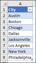
In a new worksheet, type the entries you want to appear in your drop-down list. Ideally, you’ll have your list items in an
Excel table
. If you don’t, then you can quickly convert your list to a table by selecting any cell in the range, and pressing

Ctrl+T

.
Notes:
- Why should you put your data in a table? When your data is in a table, then as you
  add or remove items from the list
  , any drop-downs you based on that table will automatically update. You don’t need to do anything else.
- Now is a good time to
  Sort data in a range or table
  in your drop-down list.
Select the cell in the worksheet where you want the drop-down list.
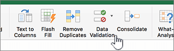
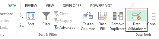
Go to the

Data

tab on the Ribbon, then

Data Validation

.

Note:
If you can’t click

Data Validation

, the worksheet might be protected or shared.
Unlock specific areas of a protected workbook
or stop sharing the worksheet, and then try step 3 again.
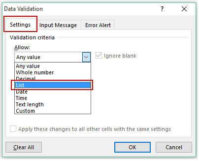
On the

Settings

tab, in the

Allow

box, click

List

.
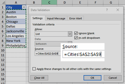
Click in the

Source

box, then select your list range. We put ours on a sheet called Cities, in range A2:A9. Note that we left out the header row, because we don’t want that to be a selection option:
If it’s OK for people to leave the cell empty, check the

Ignore blank

box.
Check the

In-cell dropdown

box.
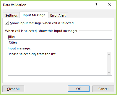
Click the

Input Message

tab.
- If you want a message to pop up when the cell is clicked, check the
  
  Show input message when cell is selected
  
  box, and type a title and message in the boxes (up to 225 characters). If you don’t want a message to show up, clear the check box.
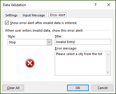
Click the

Error Alert

tab.
- If you want a message to pop up when someone enters something that’s not in your list, check the
  
  Show error alert after invalid data is entered
  
  box, pick an option from the
  
  Style
  
  box, and type a title and message. If you don’t want a message to show up, clear the check box.
Not sure which option to pick in the

Style

box?
- To show a message that doesn’t stop people from entering data that isn’t in the drop-down list, click
  
  Information
  
  or Warning. Information will show a message with this icon
  
  and Warning will show a message with this icon
  
  .
- To stop people from entering data that isn’t in the drop-down list, click
  
  Stop
  
  .
  
  Note:
  If you don’t add a title or text, the title defaults to «Microsoft Excel» and the message to: «The value you entered is not valid. A user has restricted values that can be entered into this cell.»

You can download an example workbook with multiple data validation examples like the one in this article. You can follow along, or create your own data validation scenarios.
Download Excel data validation examples
.

Data entry is quicker and more accurate when you restrict values in a cell to choices from a drop-down list.

Start by making a list of valid entries on a sheet, and sort or rearrange the entries so that they appear in the order you want. Then you can use the entries as the source for your drop-down list of data. If the list is not large, you can easily refer to it and type the entries directly into the data validation tool.

Create a list of valid entries for the drop-down list, typed on a sheet in a single column or row without blank cells.
Select the cells that you want to restrict data entry in.
On the

Data

tab, under

Tools

, click

Data Validation

or

Validate

.

Note:
If the validation command is unavailable, the sheet might be protected or the workbook may be shared. You cannot change data validation settings if your workbook is shared or your sheet is protected. For more information about workbook protection, see
Protect a workbook
.
Click the

Settings

tab, and then in the

Allow

pop-up menu, click

List

.
Click in the

Source

box, and then on your sheet, select your list of valid entries.

The dialog box minimizes to make the sheet easier to see.
Press RETURN or click the

Expand

button to restore the dialog box, and then click

OK

.
Tips:
- You can also type values directly into the
  
  Source
  
  box, separated by a comma.
- To modify the list of valid entries, simply change the values in the source list or edit the range in the
  
  Source
  
  box.
- You can specify your own error message to respond to invalid data inputs. On the
  
  Data
  
  tab, click
  
  Data Validation
  
  or
  
  Validate
  
  , and then click the
  
  Error Alert
  
  tab.

Need more help?

You can always ask an expert in the Excel Tech Community or get support in the Answers community.

About This Article

Article SummaryX

1. Double-click the cell.
2. Press Alt + 7 or Option + 8 to add a bullet point.
3. Type a list item.
4. Press Alt + Enter (PC) or Control + Option + Return (Mac) to go to the next line.
5. Repeat until your list is finished.

Did this summary help you?

Thanks to all authors for creating a page that has been read 62,222 times.

Is this article up to date?

Источник

When we need to collect data from others, they may write different things from their perspective. Still, we need to make all the related stories under one. Also, it is common that while entering the data, they make mistakes because of typo errors. For example, assume in certain cells, if we ask users to enter either “YES” or “NO,” one will enter “Y,” someone will insert “YES” like this, and we may end up getting a different kind of results. So in such cases, creating a list of values as pre-determined values allows the users only to choose from the list instead of users entering their values. Therefore, in this article, we will show you how to create a list of values in Excel.

Create List in Excel
- #1 – Create a Drop-Down List in Excel
- #2 – Create List of Values from Cells
- #3 – Create List through Named Manager
- Things to Remember
- Recommended Articles

You can download this Create List Excel Template here – Create List Excel Template

#1 – Create a Drop-Down List in Excel

We can create a drop-down list in Excel using the “Data Validation in excelThe data validation in excel helps control the kind of input entered by a user in the worksheet.read more” tool, so as the word itself says, data will be validated even before the user decides to enter. So, all the values that need to be entered are pre-validated by creating a drop-down list in Excel. For example, assume we need to allow the user to choose only “Agree” and “Not Agree,” so we will create a list of values in the drop-down list.

In the Excel worksheet under the “Data” tab, we have an option called “Data Validation” from this again, choose “Data Validation.”

As a result, this will open the “Data Validation” tool window.

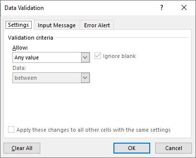
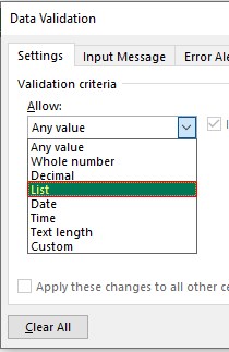
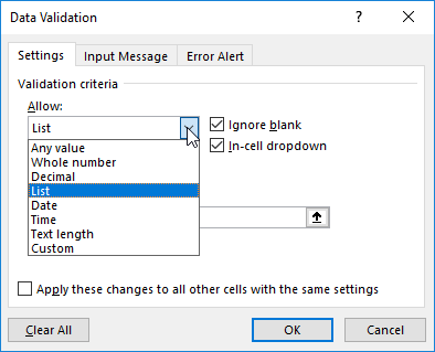
The “Settings” tab will be shown by default, and now we need to create validation criteria. Since we are creating a list of values, choose “List” as the option from the “Allow” drop-down list.

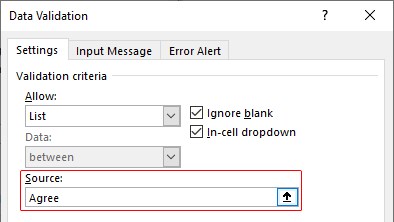
For this “List,” we can give a list of values to be validated in the following way, i.e., by directly entering the values in the “Source” list.

Enter the first value as “Agree.”

Once the first value to be validated is entered, we need to enter “comma” (,) as the list separator before entering the next value. So, enter “comma” and enter the following values as “Not Agree.”

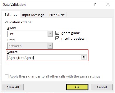
After that, click on “Ok,” and the list of values may appear in the form of the “drop-down” list.

#2 – Create a List of Values from Cells

The above method is to get started, but imagine the scenario of creating a long list of values or your list of values changing now and then. Then, it may get difficult to return and edit the list of values manually. So, by entering values in the cell, we can easily create a list of values in Excel.

Follow the steps to create a list from cell values.

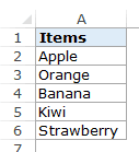
We must first insert all the values in the cells.
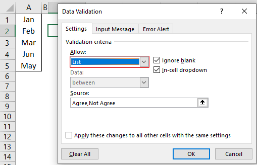
Then, open “Data Validation” and choose the validation type as “List.”
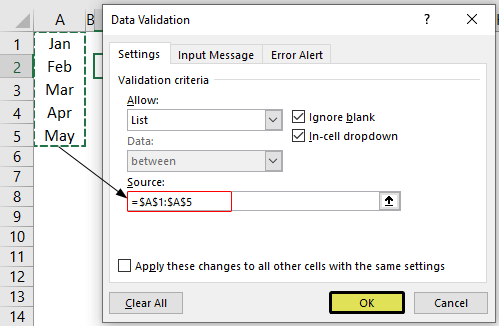
Next, in the “Source” box, we need to place the cursor and select the list of values from the range of cells A1 to A5.
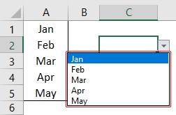
Click on “OK,” and we will have the list ready in cell C2.

So values to this list are supplied from the range of cells A1 to A5. Any changes in these referenced cells will also impact the drop-down list.

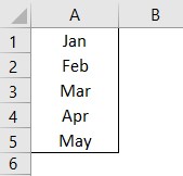
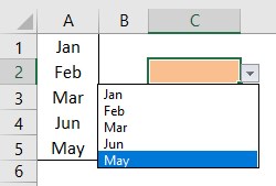
For example, in cell A4, we have a value as “Apr,” but now we will change that to “Jun” and see what happens in the drop-down list.

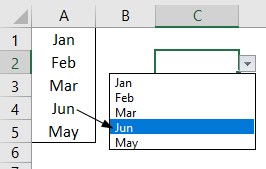
Now, look at the result of the drop-down list. Instead of “Apr,” we see “Jun” because we had given the list source as cell range, not manual entries.

#3 – Create List through Named Manager

There is another way to create a list of values, i.e., through named ranges in excelName range in Excel is a name given to a range for the future reference. To name a range, first select the range of data and then insert a table to the range, then put a name to the range from the name box on the left-hand side of the window.read more.

We have values from A1 to A5 in the above example, naming this range “Months.”

Now, select the cell where we need to create a list and open the drop-down list.

Now place the cursor in the “Source” box and press the F3 key to an open list of named ranges.

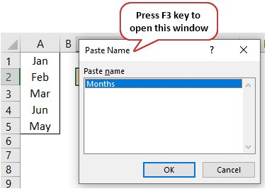
As we can see above, we have a list of names, choose the name “Months” and click on “OK” to get the name to the “Source” box.

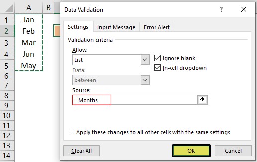
Click on “OK,” and the drop-down list is ready.

Things to Remember

The shortcut key to open data validation is “ALT + A + V + V.“
We must always create a list of values in the cells so that it may impact the drop-down list if any change happens in the referenced cells.

How to Create a Drop Down List in Excel

In this section, you will learn the exacts steps to create an Excel drop-down list:

Using Data from Cells.
Entering Data Manually.
Using the OFFSET formula.

#1 Using Data from Cells

Let’s say you have a list of items as shown below:

Here are the steps to create an Excel Drop Down List:

Select a cell where you want to create the drop down list.
Go to Data –> Data Tools –> Data Validation.
In the Data Validation dialogue box, within the Settings tab, select List as the Validation criteria.
- As soon as you select List, the source field appears.
In the source field, enter =$A$2:$A$6, or simply click in the Source field and select the cells using the mouse and click OK. This will insert a drop down list in cell C2.
- Make sure that the In-cell dropdown option is checked (which is checked by default). If this option in unchecked, the cell does not show a drop down, however, you can manually enter the values in the list.

Note: If you want to create drop down lists in multiple cells at one go, select all the cells where you want to create it and then follow the above steps. Make sure that the cell references are absolute (such as $A$2) and not relative (such as A2, or A$2, or $A2).

#2 By Entering Data Manually

In the above example, cell references are used in the Source field. You can also add items directly by entering it manually in the source field.

For example, let’s say you want to show two options, Yes and No, in the drop down in a cell. Here is how you can directly enter it in the data validation source field:

This will create a drop-down list in the selected cell. All the items listed in the source field, separated by a comma, are listed in different lines in the drop down menu.

All the items entered in the source field, separated by a comma, are displayed in different lines in the drop down list.

Note: If you want to create drop down lists in multiple cells at one go, select all the cells where you want to create it and then follow the above steps.

#3 Using Excel Formulas

Apart from selecting from cells and entering data manually, you can also use a formula in the source field to create an Excel drop down list.

Any formula that returns a list of values can be used to create a drop-down list in Excel.

For example, suppose you have the data set as shown below:

Here are the steps to create an Excel drop down list using the OFFSET function:

This will create a drop-down list that lists all the fruit names (as shown below).

Note: If you want to create a drop-down list in multiple cells at one go, select all the cells where you want to create it and then follow the above steps. Make sure that the cell references are absolute (such as $A$2) and not relative (such as A2, or A$2, or $A2).

How this formula Works??

In the above case, we used an OFFSET function to create the drop down list. It returns a list of items from the ra

It returns a list of items from the range A2:A6.

Here is the syntax of the OFFSET function: =OFFSET(reference, rows, cols, [height], [width])

It takes five arguments, where we specified the reference as A2 (the starting point of the list). Rows/Cols are specified as 0 as we don’t want to offset the reference cell. Height is specified as 5 as there are five elements in the list.

Now, when you use this formula, it returns an array that has the list of the five fruits in A2:A6. Note that if you enter the formula in a cell, select it and press F9, you would see that it returns an array of the fruit names.

Creating a Dynamic Drop Down List in Excel (Using OFFSET)

The above technique of using a formula to create a drop down list can be extended to create a dynamic drop down list as well. If you use the OFFSET function, as shown above, even if you add more items to the list, the drop down would not update automatically. You will have to manually update it each time you change the list.

Here is a way to make it dynamic (and it’s nothing but a minor tweak in the formula):

Select a cell where you want to create the drop down list (cell C2 in this example).
Go to Data –> Data Tools –> Data Validation.
In the Data Validation dialogue box, within the Settings tab, select List as the Validation criteria. As soon as you select List, the source field appears.
In the source field, enter the following formula: =OFFSET($A$2,0,0,COUNTIF($A$2:$A$100,”<>”))
Make sure that the In-cell drop down option is checked.
Click OK.

In this formula, I have replaced the argument 5 with COUNTIF($A$2:$A$100,”<>”).

The COUNTIF function counts the non-blank cells in the range A2:A100. Hence, the OFFSET function adjusts itself to include all the non-blank cells.

Note:

For this to work, there must NOT be any blank cells in between the cells that are filled.
If you want to create a drop-down list in multiple cells at one go, select all the cells where you want to create it and then follow the above steps. Make sure that the cell references are absolute (such as $A$2) and not relative (such as A2, or A$2, or $A2).

Copy Pasting Drop-Down Lists in Excel

You can copy paste the cells with data validation to other cells, and it will copy the data validation as well.

For example, if you have a drop-down list in cell C2, and you want to apply it to C3:C6 as well, simply copy the cell C2 and paste it in C3:C6. This will copy the drop-down list and make it available in C3:C6 (along with the drop down, it will also copy the formatting).

If you only want to copy the drop down and not the formatting, here are the steps:

This will only copy the drop down and not the formatting of the copied cell.

Caution while Working with Excel Drop Down List

You need to to be careful when you are working with drop down lists in Excel.

When you copy a cell (that does not contain a drop down list) over a cell that contains a drop down list, the drop down list is lost.

The worst part of this is that Excel will not show any alert or prompt to let the user know that a drop down will be overwritten.

How to Select All Cells that have a Drop Down List in it

Sometimes, it ‘s hard to know which cells contain the drop down list.

Hence, it makes sense to mark these cells by either giving it a distinct border or a background color.

Instead of manually checking all the cells, there is a quick way to select all the cells that have drop-down lists (or any data validation rule) in it.

This would instantly select all the cells that have a data validation rule applied to it (this includes drop down lists as well).

Now you can simply format the cells (give a border or a background color) so that visually visible and you don’t accidentally copy another cell on it.

Here is another technique by Jon Acampora you can use to always keep the drop down arrow icon visible. You can also see some ways to do this in this video by Mr. Excel.

Creating a Dependent / Conditional Excel Drop Down List

Here is a video on how to create a dependent drop-down list in Excel.

If you prefer reading over watching a video, keep reading.

Sometimes, you may have more than one drop-down list and you want the items displayed in the second drop down to be dependent on what the user selected in the first drop-down.

These are called dependent or conditional drop down lists.

Below is an example of a conditional/dependent drop down list:

In the above example, when the items listed in ‘Drop Down 2’ are dependent on the selection made in ‘Drop Down 1’.

Now let’s see how to create this.

Here are the steps to create a dependent / conditional drop down list in Excel:

Now, when you make the selection in Drop Down 1, the options listed in Drop Down List 2 would automatically update.

Download the Example File

How does this work? – The conditional drop down list (in cell E3) refers to =INDIRECT(D3). This means that when you select ‘Fruits’ in cell D3, the drop down list in E3 refers to the named range ‘Fruits’ (through the INDIRECT function) and hence lists all the items in that category.

Important Note While Working with Conditional Drop Down Lists in Excel:

When you have made the selection, and then you change the parent drop down, the dependent drop down would not change and would, therefore, be a wrong entry. For example, if you select the US as the country and then select Florida as the state, and then go back and change the country to India, the state would remain as Florida. Here is a great tutorial by Debra on clearing dependent (conditional) drop down lists in Excel when the selection is changed.
If the main category is more than one word (for example, ‘Seasonal Fruits’ instead of ‘Fruits’), then you need to use the formula =INDIRECT(SUBSTITUTE(D3,” “,”_”)), instead of the simple INDIRECT function shown above. The reason for this is that Excel does not allow spaces in named ranges. So when you create a named range using more than one word, Excel automatically inserts an underscore in between words. So ‘Seasonal Fruits’ named range would be ‘Seasonal_Fruits’. Using the SUBSTITUTE function within the INDIRECT function makes sure that spaces are converted into underscores.

You May Also Like the Following Excel Tutorials:

Extract Data from Drop Down List Selection in Excel.
Select Multiple Items from a Drop Down List in Excel.
Creating a Dynamic Excel Filter Search Box.
Display Main and Subcategory in Drop Down List in Excel.
How to Insert Checkbox in Excel.
Using a Radio Button (Option Button) in Excel.
How to Remove Drop-Down List in Excel?

Источник

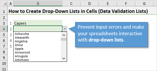
Bottom Line: The complete Excel guide on how to create drop-down lists in cells (data validation lists). Includes keyboard shortcuts to select items, copying drop-downs to other cells, handling invalid inputs, updating lists with new items, and more.

Skill Level: Beginner

Watch on YouTube & Subscribe to our Channel

Download the Excel File

You can download the file I’m using in the video here:

What Are Data Validation Lists?

Creating a drop-down list is a great way to ensure that entries are uniform and free from spelling errors. It also helps restrict entries so that only values you’ve approved make it onto the sheet.

That’s why they are also called data validation lists. They help to make sure that only valid data makes it into the cells that you’ve applied it to.

This can be helpful when multiple users are entering data on the same sheet and you want the options to be limited to a list of items or values that you’ve already approved.

We can also use drop-down lists to create interactive reports and financial models, where results change when the user changes a cell’s value.

How to Create a Drop-down (Data Validation) List

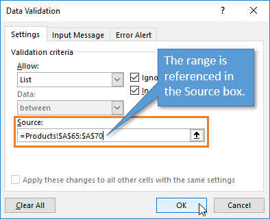
To create a drop-down list, start by going to the Data tab on the Ribbon and click the Data Validation button.

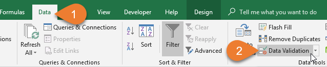
The Data Validation window will appear. The keyboard shortcut to open the Data Validation window is Alt, A, V, V.

You’ll want to select List in the drop-down menu under Allow.

At this point there are a few ways that you can tell Excel what items you want to include in your drop-down list.

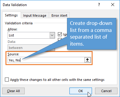
Drop-down List from Comma Separated Values

The first way is by typing all of the options that you want in your drop-down list, separated by commas, into the Source field. For example, if there are only two options to choose from, such as Yes and No, you would simply type “Yes, No” (do not include the quotation marks) in the Source box. It doesn’t matter whether a space follows your comma or not.

A longer list of options might look like this: “Red, Blue, Green, Purple, Orange, Yellow, Brown”. The options in your drop-down list will appear in the exact same order that you have typed them.

Note: On some language versions of Excel you will need to use a semicolon (;) instead of a comma.

Drop-down List from a Range of Values

The second way to fill your list with options is to choose them from a range of values. To do this, instead of typing values into the Source field, you want to select the icon to the right.

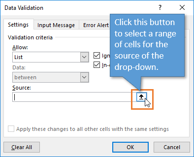
Selecting this icon will open up a small window that will auto-fill when you select a range of cells on the worksheet. Once you’ve selected the values you want to appear in your drop-down list, you can click on the corresponding icon to take you back to the Data Validation window.

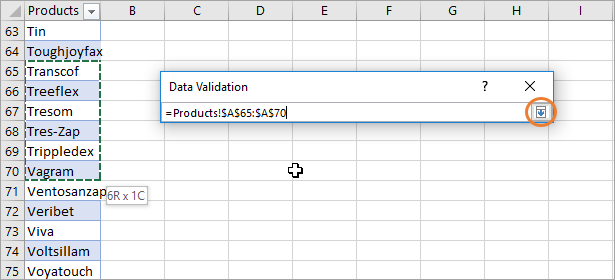
At this point, the range you’ve selected will show in the Source box and you can just hit OK.

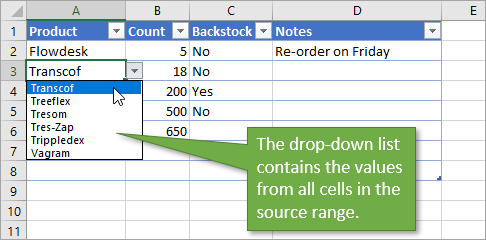
Now the values in the range that you’ve selected show as options that you can choose from in your drop-down list.

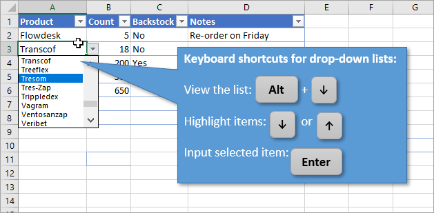
Shortcut for Selecting from the Drop-down List

To choose the option you want from your drop-down list, you can use your mouse to click on the option you want. Another way to select it is to use the keyboard shortcut Alt+?. This brings up the drop-down list and you can use your up and down arrow keys to highlight the selection you want, and then press Enter to select.

How to Search the Drop-down List

Unfortunately, Excel doesn’t have an option to search the drop-down list for a particular item, but I’ve created an add-in that gives you that option. It’s called List Search and you can access that add-in here:

Click here to download the List Search Add-in

Note: You will create a free account for the Excel Campus Members site to access the download and any future updates. The download site also contains installation instructions and videos.

How to Copy the Data Validation List to Other Cells

If you have created a drop-down list for a particular cell and would like other cells to have the same data validation list, you can easily copy (extend) that list to other cells.

Start by clicking on the cell that has the list, and then select any additional cells that you want to extend the drop-down list to. This can include blank cells or cells that already have values in them.

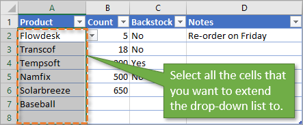
As before, you will click on the Data Validation button in the Data tab, but this time a warning will appear that says, “The selection contains some cells without Data Validation settings. Do you want to extend the Data Validation to these cells?”

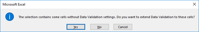
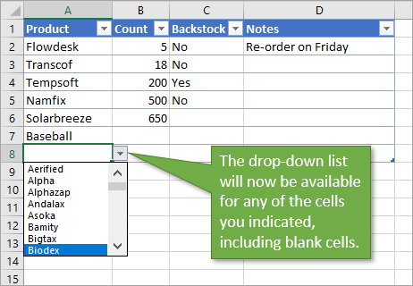
Choose Yes, and then hit OK when the Data Validation Window appears. You’ll see that each of the cells in your selection now has the same drop-down options as the original cell.

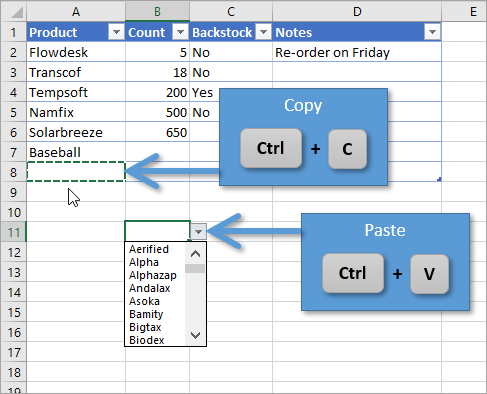
It’s also worth noting that you can copy and paste Data Validation from one cell to another just as you would copy and paste normal values and formatting.

Handling Errors and Invalid Inputs

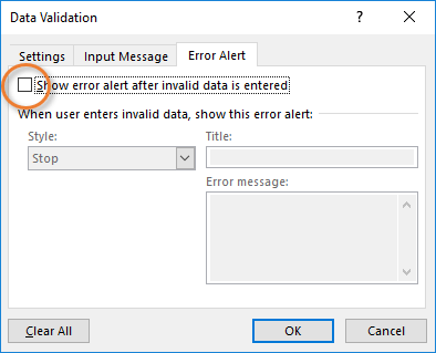
What happens when we enter a value into a cell that has a Data Validation List, but that value is not one of the options in the list? That depends on the Error Alert settings, which we have control of.

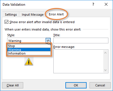
To change the kind of message the user receives when they enter an extraneous value, you can go back to the Data Validation window. Under the Error Alert tab, you can find three options: Stop, Warning, and Information.

You’ll also notice that there are fields where you can change the title of the error message and the text of the message itself, so that when the user enters data that’s not part of your validation list, they will receive an alert that’s worded in the way you want it to appear.

Here is an explanation of each Error Alert Style:

Stop Style

When the user types an invalid entry, an error message will appear that gives the option to either retype the entry or cancel the attempt. The message looks like this:

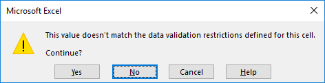
Warning Style

The Warning style displays a message that gives the user a choice to allow an entry that isn’t on the preset list.

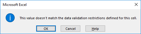
Information Style

The Information style displays a message that automatically allows the entry no matter what the value is. The user is presented with informative text about validation rules.

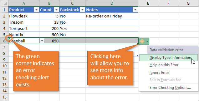
Error Checking Alert

When any invalid entry is made in a cell, the error checking alert will appear in the cell. The error is indicated with the green triangle in the top-left corner of the cell. Clicking the Error Box button will allow you to see more info about data validation error. You can select “Display Type Information” from the list to see the cause of the error.

Disable Error Alerts

Another option under the Error Alert tab is to uncheck the box that says, “Show error alert after invalid data is entered.” This allows any value to be entered into the cell, and no message box will appear.

Adding New Data to the Source Range of the List

Adding new options to our drop-down list is possible, but it isn’t automatic when we add new items the bottom of our source list. We need to tell Excel what our new extended source range is. You can do that in the Data Validation window by just typing in the new range, or re-selecting the range to include the new data. (See the section above entitled “Create a Drop-Down List from a Range of Values” for how to select your range.)

The great thing is that we don’t have to redefine these settings for each cell that has Data Validation. The “Apply these changes to all other cells with the same settings” checkbox does this for us. When you click the checkbox, the other cells will selected in the background. This gives you a visual indication of what will be updated.

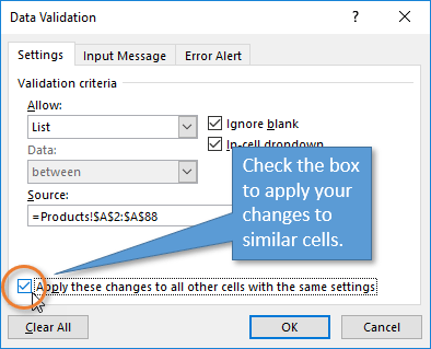
Then press OK. Any cells that shared the same data validation settings will now include the updated changes that you’ve made.

There is a way to automate the process so that any change you make to the source data instantly updates your drop-down list. It involves using Excel tables and named ranges. You can find out how in this post:

How to Add New Rows to Drop-down Lists Automatically – Dynamic Data Validation Lists

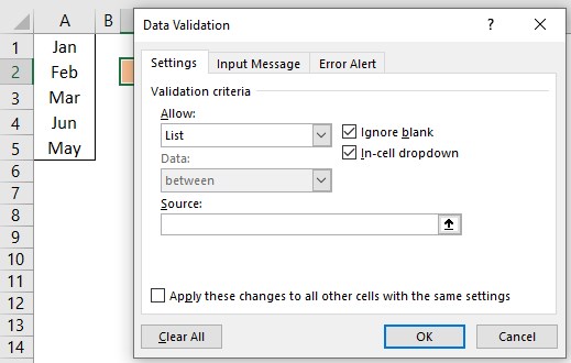
Removing Data Validation from a Cell

Getting rid of a Data Validation list is simple. Open the Data Validation window and click the Clear All button.

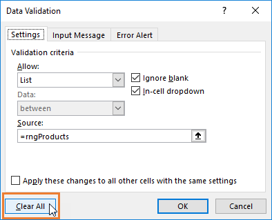
If you want to clear the validation settings from other cells with the same settings, make sure to click that checkbox before hitting the Clear All button.

Make Your Workbooks Interactive

Data Validation lists are a great tool to add to your Excel toolbelt. They help us keep our data clean and make our spreadsheets easier to use. We can use them as the source of lookup formulas to create interactive financial models and reports. I will do some follow-up posts with these techniques as well.

Once you feel comfortable with drop-down lists, you may want to try dependent (also called cascading) lists. These are lists that change depending on what you’ve already chosen in another list. For example, you may create a list of car brands, like Toyota, Ford, and Honda. Then you can have a second list of car models that populates with specific options depending on what you choose in the first list. If you choose Toyota in the first list, you might see Corolla, Camry, and Tacoma in the second. But if you go back to the first list and choose Ford, the options in the second list can change to Mustang, Explorer, and Focus. Learn how to create dependent cascading lists here.

If you have any questions or comments about how to use drop-down lists, don’t hesitate to leave a comment below. Thanks! 😊

Источник

Create a drop-down list

See also

Need more help?

See also

Need more help?

About This Article

Is this article up to date?

Table of contents

#1 – Create a Drop-Down List in Excel

#2 – Create a List of Values from Cells

#3 – Create List through Named Manager

Things to Remember

Recommended Articles

How to Create a Drop Down List in Excel

#1 Using Data from Cells

#2 By Entering Data Manually

#3 Using Excel Formulas

Creating a Dynamic Drop Down List in Excel (Using OFFSET)

Copy Pasting Drop-Down Lists in Excel

Caution while Working with Excel Drop Down List

How to Select All Cells that have a Drop Down List in it

Creating a Dependent / Conditional Excel Drop Down List

Download the Excel File

What Are Data Validation Lists?

How to Create a Drop-down (Data Validation) List

Drop-down List from Comma Separated Values

Drop-down List from a Range of Values

Shortcut for Selecting from the Drop-down List

How to Search the Drop-down List

How to Copy the Data Validation List to Other Cells

Handling Errors and Invalid Inputs

Stop Style

Warning Style

Information Style

Error Checking Alert

Adding New Data to the Source Range of the List

Removing Data Validation from a Cell

Make Your Workbooks Interactive