
If you use Excel on a daily basis, then you’ve probably run into situations where you needed to hide something in your Excel worksheet. Maybe you have some extra data worksheets that are referenced, but don’t need to be viewed. Or maybe you have a few rows of data at the bottom of the worksheet that need to be hidden.
There are a lot of different parts to an Excel spreadsheet and each part can be hidden in different ways. In this article, I’ll walk you through the different content that can be hidden in Excel and how to get view the hidden data at a later time.
How to Hide Tabs/WorkSheets
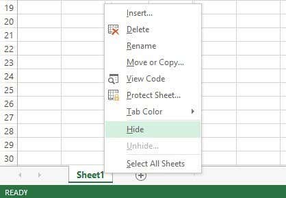
In order to hide a worksheet or tab in Excel, right-click on the tab and choose Hide. That was pretty straightforward.
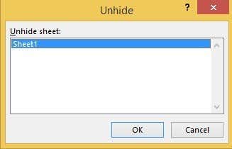
Once hidden, you can right-click on a visible sheet and select Unhide. All hidden sheets will be shown in a list and you can select the one you want to unhide.
Excel does not have the ability to hide a cell in the traditional sense that they simply disappear until you unhide them, like in the example above with sheets. It can only blank out a cell so that it appears that nothing is in the cell, but it can’t truly “hide” a cell because if a cell is hidden, what would you replace that cell with?
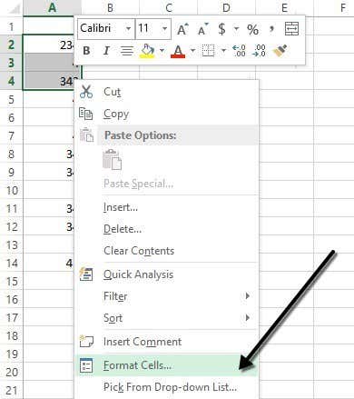
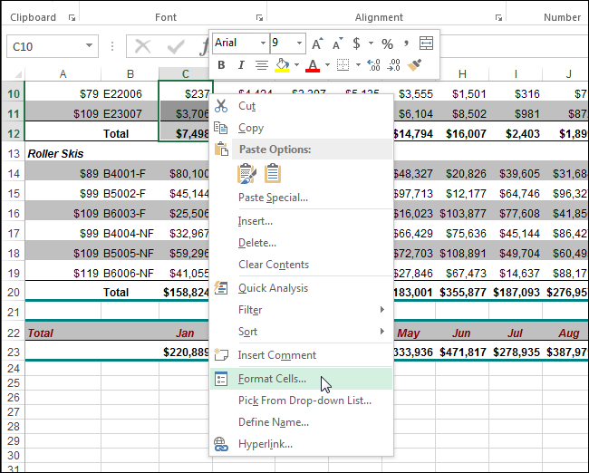
You can hide entire rows and columns in Excel, which I explain below, but you can only blank out individual cells. Right-click on a cell or multiple selected cells and then click on Format Cells.
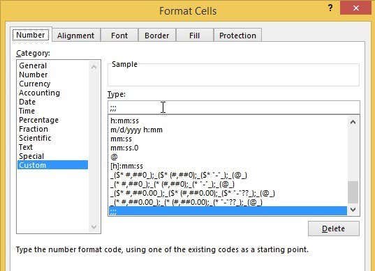
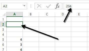
On the Number tab, choose Custom at the bottom and enter three semicolons (;;;) without the parentheses into the Type box.
Click OK and now the data in those cells is hidden. You can click on the cell and you should see the cell remains blank, but the data in the cell shows up in the formula bar.
To unhide the cells, follow the same procedure above, but this time choose the original format of the cells rather than Custom. Note that if you type anything into those cells, it will automatically be hidden after you press Enter. Also, whatever original value was in the hidden cell will be replaced when typing into the hidden cell.
Hide Gridlines
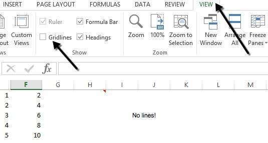
A common task in Excel is hiding gridlines to make the presentation of the data cleaner. When hiding gridlines, you can either hide all gridlines on the entire worksheet or you can hide gridlines for a certain portion of the worksheet. I will explain both options below.
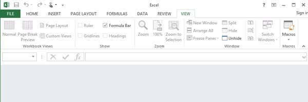
To hide all gridlines, you can click on the View tab and then uncheck the Gridlines box.
You can also click on the Page Layout tab and uncheck the View box under Gridlines.

How to Hide Rows and Columns
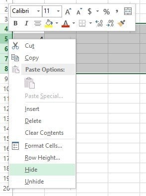
If you want to hide an entire row or column, right-click on the row or column header and then choose Hide. To hide a row or multiple rows, you need to right-click on the row number at the far left. To hide a column or multiple columns, you need to right-click on the column letter at the very top.
You can easily tell there are hidden rows and columns in Excel because the numbers or letters skip and there are two visible lines shown to indicate hidden columns or rows.
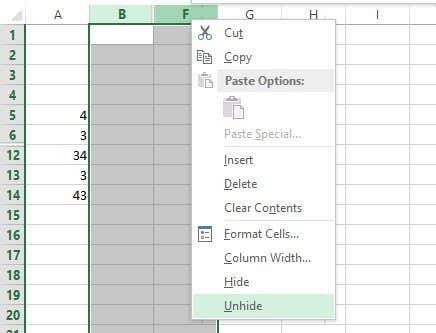
To unhide a row or column, you need to select the row/column before and the row/column after the hidden row/column. For example, if Column B is hidden, you would need to select column A and column C and then right-click and choose Unhide to unhide it.
How to Hide Formulas
Hiding formulas is slightly more complicated than hiding rows, columns, and tabs. If you want to hide a formula, you have to do TWO things: set the cells to Hidden and then protect the sheet.
So, for example, I have a sheet with some proprietary formulas that I don’t want anyone to see!

First, I will select the cells in column F, right-click and choose Format Cells. Now click on the Protection tab and check the box that says Hidden.
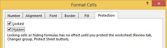
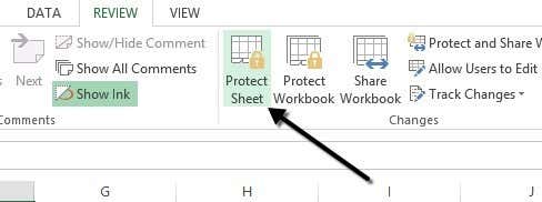
As you can see from the message, hiding formulas won’t go into effect until you actually protect the worksheet. You can do this by clicking on the Review tab and then clicking on Protect Sheet.
You can enter in a password if you want to prevent people from un-hiding the formulas. Now you’ll notice that if you try to view the formulas, by pressing CTRL + ~ or by clicking on Show Formulas on the Formulas tab, they will not be visible, however, the results of that formula will remain visible.
Hide Comments
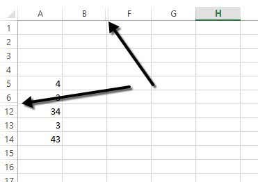
By default, when you add a comment to an Excel cell, it will show you a small red arrow in the upper right corner to indicate there is a comment there. When you hover over the cell or select it, the comment will appear in a pop up window automatically.
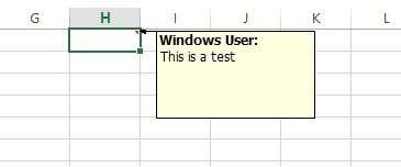
You can change this behavior so that the arrow and the comment are not shown when hovering or selecting the cell. The comment will still remain and can be viewed by simply going to the Review tab and clicking on Show All Comments. To hide the comments, click on File and then Options.
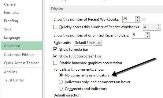
Click on Advanced and then scroll down to the Display section. There you will see an option called No comment or indicators under the For cells with comments, show: heading.
Hide Overflow Text
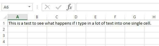
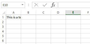
In Excel, if you type a lot of text into a cell, it will simply overflow over the adjacent cells. In the example below, the text only exists in cell A1, but it overflows to other cells so that you can see it all.
If I were to type something into cell B1, it would then cut off the overflow and show the contents of B1. If you want this behavior without having to type anything into the adjacent cell, you can right-click on the cell, choose Format Cells and then select Fill from the Horizontal Text alignment drop down box.
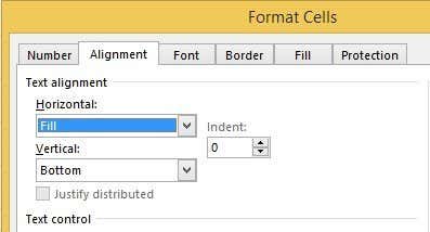
This will hide the overflow text for that cell even if nothing is in the adjacent cell. Note that this is kind of a hack, but it works most of the time.
You could also choose Format Cells and then check the Wrap Text box under Text control on the Alignment tab, but that will increase the height of the row. To get around that, you could simply right-click on the row number and then click on Row Height to adjust the height back to its original value. Either of these two methods will work for hiding overflow text.
Hide Workbook
I’m not sure why you would want or need to do this, but you can also click on the View tab and click on the Hide button under Split. This will hide the entire workbook in Excel! There is absolutely nothing you can do other than clicking on the Unhide button to bring back the workbook.
So now you’ve learnt how to hide workbooks, sheets, rows, columns, gridlines, comments, cells, and formulas in Excel! If you have any questions, post a comment. Enjoy!
Locate hidden cells
Follow these steps:
-
Select the worksheet containing the hidden rows and columns that you need to locate, then access the Special feature with one of the following ways:
-
Press F5 > Special.
-
Press Ctrl+G > Special.
-
Or on the Home tab, in the Editing group, click Find & Select>Go To Special.
-
-
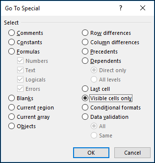
Under Select, click Visible cells only, and then click OK.

All visible cells are selected and the borders of rows and columns that are adjacent to hidden rows and columns will appear with a white border.
Note: Click anywhere on the worksheet to cancel the selection of the visible cells. If the hidden cells that you need to reveal are outside the visible worksheet area, use the scroll bars to move through the document until the hidden rows and columns that contain those cells are visible.
This feature is not available in Excel for the web.
Learn several ways to do this
Updated on September 19, 2022
What to Know
- Hide a column: Select a cell in the column to hide, then press Ctrl+0. To unhide, select an adjacent column and press Ctrl+Shift+0.
- Hide a row: Select a cell in the row you want to hide, then press Ctrl+9. To unhide, select an adjacent column and press Ctrl+Shift+9.
- You can also use the right-click context menu and the format options on the Home tab to hide or unhide individual rows and columns.
You can hide columns and rows in Excel to make a cleaner worksheet without deleting data you might need later, although there is no way to hide individual cells. In this guide, we provide instructions for three ways to hide and unhide columns in Excel 2019, 2016, 2013, 2010, 2007, and Excel for Microsoft 365.
Hide Columns in Excel Using a Keyboard Shortcut
The keyboard key combination for hiding columns is Ctrl+0.
-
Click on a cell in the column you want to hide to make it the active cell.
-
Press and hold down the Ctrl key on the keyboard.
-
Press and release the 0 key without releasing the Ctrl key. The column containing the active cell should be hidden from view.
To hide multiple columns using the keyboard shortcut, highlight at least one cell in each column to be hidden, and then repeat steps two and three above.
Hide Columns Using the Context Menu
The options available in the context — or right-click menu — change depending upon the object selected when you open the menu. If the Hide option, as shown in the image below, is not available in the context menu it is likely that you didn’t select the entire column before right-clicking.
Hide a Single Column
-
Click the column header of the column you want to hide to select the entire column.
-
Right-click on the selected column to open the context menu.
-
Choose Hide. The selected column, the column letter, and any data in the column will be hidden from view.
Hide Adjacent Columns
-
In the column header, click and drag with the mouse pointer to highlight all three columns.
-
Right-click on the selected columns.
-
Choose Hide. The selected columns and column letters will be hidden from view.
When you hide columns and rows containing data, it does not delete the data, and you can still reference it in formulas and charts. Hidden formulas containing cell references will update if the data in the referenced cells changes.
Hide Separated Columns
-
In the column header click on the first column to be hidden.
-
Press and hold down the Ctrl key on the keyboard.
-
Continue to hold down the Ctrl key and click once on each additional column to be hidden to select them.
-
Release the Ctrl key.
-
In the column header, right-click on one of the selected columns and choose Hide. The selected columns and column letters will be hidden from view.
When hiding separate columns, if the mouse pointer is not over the column header when you click the right mouse button, the hide option will not be available.
Hide and Unhide Columns in Excel Using the Name Box
This method can be used to unhide any single column. In our example, we will be using column A.
-
Type the cell reference A1 into the Name Box.
-
Press the Enter key on the keyboard to select the hidden column.
-
Click on the Home tab of the ribbon.
-
Click on the Format icon on the ribbon to open the drop-down.
-
In the Visibility section of the menu, choose Hide & Unhide > Hide Columns or Unhide Column.
Unhide Columns Using a Keyboard Shortcut
The key combination for unhiding columns is Ctrl+Shift+0.
-
Type the cell reference A1 into the Name Box.
-
Press the Enter key on the keyboard to select the hidden column.
-
Press and hold down the Ctrl and the Shift keys on the keyboard.
-
Press and release the 0 key without releasing the Ctrl and Shift keys.
To unhide one or more columns, highlight at least one cell in the columns on either side of the hidden column(s) with the mouse pointer.
-
Click and drag with the mouse to highlight columns A to G.
-
Press and hold down the Ctrl and the Shift keys on the keyboard.
-
Press and release the 0 key without releasing the Ctrl and Shift keys. The hidden column(s) will become visible.
The Ctrl+Shift+0 keyboard shortcut might not work depending on the version of Windows you’re running, for reasons not explained by Microsoft. If this shortcut doesn’t work, use another method from the article.
Unhide Columns Using the Context Menu
As with the shortcut key method above, you must select at least one column on either side of a hidden column or columns to unhide them. For example, to unhide columns D, E, and G:
-
Hover the mouse pointer over column C in the column header. Click and drag with the mouse to highlight columns C to H to unhide all columns at one time.
-
Right-click on the selected columns and choose Unhide. The hidden column(s) will become visible.
Hide Rows Using Shortcut Keys
The keyboard key combination for hiding rows is Ctrl+9:
-
Click on a cell in the row you want to hide to make it the active cell.
-
Press and hold down the Ctrl key on the keyboard.
-
Press and release the 9 key without releasing the Ctrl key. The row containing the active cell should be hidden from view.
To hide multiple rows using the keyboard shortcut, highlight at least one cell in each row you want to hide, and then repeat steps two and three above.
Hide Rows Using the Context Menu
The options available in the context menu — or right-click — change depending upon the object selected when you open it. If the Hide option, as shown in the image above, is not available in the context menu it is because you probably didn’t select the entire row.
Hide a Single Row
-
Click on the row header for the row to be hidden to select the entire row.
-
Right-click on the selected row to open the context menu.
-
Choose Hide. The selected row, the row letter, and any data in the row will be hidden from view.
Hide Adjacent Rows
-
In the row header, click and drag with the mouse pointer to highlight all three rows.
-
Right-click on the selected rows and choose Hide. The selected rows will be hidden from view.
Hide Separated Rows
-
In the row header, click on the first row to be hidden.
-
Press and hold down the Ctrl key on the keyboard.
-
Continue to hold down the Ctrl key and click once on each additional row to be hidden to select them.
-
Right-click on one of the selected rows and choose Hide. The selected rows will be hidden from view.
Hide and Unhide Rows Using the Name Box
This method can be used to unhide any single row. In our example, we will be using row 1.
-
Type the cell reference A1 into the Name Box.
-
Press the Enter key on the keyboard to select the hidden row.
-
Click on the Home tab of the ribbon.
-
Click on the Format icon on the ribbon to open the drop-down menu.
-
In the Visibility section of the menu, choose Hide & Unhide > Hide Rows or Unhide Row.
Unhide Rows Using a Keyboard Shortcut
The key combination for unhiding rows is Ctrl+Shift+9.
Unhide Rows using Shortcut Keys and Name Box
-
Type the cell reference A1 into the Name Box.
-
Press the Enter key on the keyboard to select the hidden row.
-
Press and hold down the Ctrl and the Shift keys on the keyboard.
-
Press and hold down the Ctrl and the Shift keys on the keyboard. Row 1 will become visible.
Unhide Rows Using a Keyboard Shortcut
To unhide one or more rows, highlight at least one cell in the rows on either side of the hidden row(s) with the mouse pointer. For example, you want to unhide rows 2, 4, and 6.
-
To unhide all rows, click and drag with the mouse to highlight rows 1 to 7.
-
Press and hold down the Ctrl and the Shift keys on the keyboard.
-
Press and release the number 9 key without releasing the Ctrl and Shift keys. The hidden row(s) will become visible.
Unhide Rows Using the Context Menu
As with the shortcut key method above, you must select at least one row on either side of a hidden row or rows to unhide them. For example, to unhide rows 3, 4, and 6:
-
Hover the mouse pointer over row 2 in the row header.
-
Click and drag with the mouse to highlight rows 2 to 7 to unhide all rows at one time.
-
Right-click on the selected rows and choose Unhide. The hidden row(s) will become visible.
How to Move Columns in Excel
FAQ
-
How do I hide cells in Excel?
Select the cell or cells you want to hide, then select the Home tab > Cells > Format > Format Cells. In the Format Cells menu, select the Number tab > Custom (under Category) and type ;;; (three semicolons), then select OK.
-
How do I hide gridlines in Excel?
Select the Page Layout tab, then turn off the View checkbox under Gridlines.
-
How do I hide formulas in Excel?
Select the cells with formulas you want to hide > select the Hidden checkbox on the Protection tab > OK > Review > Protect Sheet. Next, verify that Protect worksheet and contents of locked cells is turned on, then select OK.
Thanks for letting us know!
Get the Latest Tech News Delivered Every Day
Subscribe

There may be times when you want to hide information in certain cells or hide entire rows or columns in an Excel worksheet. Maybe you have some extra data you reference in other cells that does not need to be visible.
We will show you how to hide cells and rows and columns in your worksheets and then show them again.
Update, 11/3/21: Looking to hide or unhide columns in Microsoft Excel? We have an updated guide for you.
RELATED: How to Hide or Unhide Columns in Microsoft Excel
Hide Cells
You can’t hide a cell in the sense that it completely disappears until you unhide it. With what would that cell be replaced? Excel can only blank out a cell so that nothing displays in the cell. Select individual cells or multiple cells using the “Shift” and “Ctrl” keys, just like you would when selecting multiple files in Windows Explorer. Right-click on any of the selected cells and select “Format Cells” from the popup menu.

The “Format Cells” dialog box displays. Make sure the “Number” tab is active and select “Custom” in the “Category” list. In the “Type” edit box, enter three semicolons (;) without the parentheses and click “OK”.
NOTE: You might want to note what the “Type” was for each of the selected cells is before you change it so you can change the type of the cells back to what it was to show the content again.
The data in the selected cells is now hidden, but the value or the formula is still in the cell and displays in the “Formula Bar”.
To unhide the content in the cells, follow the same steps listed above, but choose the original number category and type for the cells rather than “Custom” and the three semicolons.
NOTE: If you type anything into cells in which you hid the content, it will automatically be hidden after you press “Enter”. Also, the original value in the hidden cell will be replaced with the new value or formula that you type into the cell.
Hide Rows and Columns
If you have a large worksheet, you might want to hide some rows and columns for data you don’t currently need to view. To hide an entire row, right-click on the row number and select “Hide”.
NOTE: To hide multiple rows, select the rows first by clicking and dragging over the range of rows you want to hide, and then right-click on the selected rows and select “Hide”. You can select non-sequential rows by pressing “Ctrl” as you click on the row numbers for the rows you want to select.
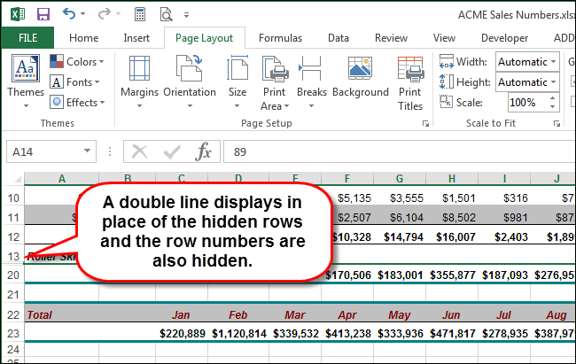
The hidden row numbers are skipped in the row number column and a double line displays in place of the hidden rows.
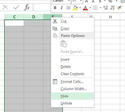
Hiding columns is a very similar process to hiding rows. Right-click on the column you want to hide, or select multiple column letters first and then right-click on the selected columns. Select “Hide” from the popup menu.
The hidden column letters are skipped in the row number column and a double line displays in place of the hidden rows.
To unhide a row or multiple rows, select the row before the hidden row(s) and the row after the hidden row(s) and right-click on the selection and select “Unhide” from the popup menu.
To unhide a column or multiple columns, select the two columns surrounding the hidden column(s), right-click on the selection, and select “Unhide” from the popup menu.
If you have a large spreadsheet and you don’t want to hide any cells, rows, or columns, you can freeze rows and columns so any headings you set up don’t scroll when you scroll through your data.
READ NEXT
- › How to Add and Remove Columns and Rows in Microsoft Excel
- › How to Copy and Paste Only Visible Cells in Microsoft Excel
- › How to Set Row Height and Column Width in Excel
- › How to Remove Blank Rows in Excel
- › How to Insert a Picture in Microsoft Excel
- › How to Use Custom Views in Excel to Save Your Workbook Settings
- › How to Count Checkboxes in Microsoft Excel
- › This New Google TV Streaming Device Costs Just $20
How-To Geek is where you turn when you want experts to explain technology. Since we launched in 2006, our articles have been read billions of times. Want to know more?
Содержание
- Hide or display cell values
- Hide cell values
- Display hidden cell values
- How to Hide Cells, Rows, and Columns in Excel
- Hide Cells
- Hide Rows and Columns
- How to hide and unhide rows in Excel
- How to hide rows in Excel
- Hide rows using the ribbon
- Hide rows using the right-click menu
- Excel shortcut to hide row
- How to unhide rows in Excel
- Unhide rows by using the ribbon
- Unhide rows using the context menu
- Unhide rows with a keyboard shortcut
- Show hidden rows by double-clicking
- How to unhide all rows in Excel
- How to unhide all cells in Excel
- How to unhide specific rows in Excel
- How to unhide top rows in Excel
- Tips and tricks for hiding and unhiding rows in Excel
- How to hide rows containing blank cells
- How to hide rows based on cell value
- Hide unused rows so that only working area is visible
- How to locate all hidden rows on a sheet
- How to copy visible rows in Excel
- Cannot unhide rows in Excel
- 1. The worksheet is protected
- 2. Row height is small, but not zero
- 3. Trouble unhiding the first row in Excel
- 4. Some rows are filtered out
Hide or display cell values
Suppose you have a worksheet that contains confidential information, such as employee salaries, that you do not want a co-worker who stops by your desk to see. Or perhaps you multiply the values in a range of cells by the value in another cell that you do not want to be visible on the worksheet. By applying a custom number format, you can hide the values of those cells on the worksheet.
Note: Although cells with hidden values appear blank on the worksheet, their values remain displayed in the formula bar where you can work with them.
Hide cell values
Select the cell or range of cells that contains values that you want to hide. For more information, see Select cells, ranges, rows, or columns on a worksheet .
Note: The selected cells will appear blank on the worksheet, but a value appears in the formula bar when you click one of the cells.
On the Home tab, click the Dialog Box Launcher  next to Number.
In the Category box, click Custom.
In the Type box, select the existing codes.
Type ;;; (three semicolons).
Tip: To cancel a selection of cells, click any cell on the worksheet.
Select the cell or range of cells that contains values that are hidden. For more information, see Select cells, ranges, rows, or columns on a worksheet .
On the Home tab, click the Dialog Box Launcher next to Number.
In the Category box, click General to apply the default number format, or click the date, time, or number format that you want.
Tip: To cancel a selection of cells, click any cell on the worksheet.
Источник
How to Hide Cells, Rows, and Columns in Excel
Lori Kaufman is a technology expert with 25 years of experience. She’s been a senior technical writer, worked as a programmer, and has even run her own multi-location business. Read more.

There may be times when you want to hide information in certain cells or hide entire rows or columns in an Excel worksheet. Maybe you have some extra data you reference in other cells that does not need to be visible.
We will show you how to hide cells and rows and columns in your worksheets and then show them again.
Update, 11/3/21: Looking to hide or unhide columns in Microsoft Excel? We have an updated guide for you.
Hide Cells
You can’t hide a cell in the sense that it completely disappears until you unhide it. With what would that cell be replaced? Excel can only blank out a cell so that nothing displays in the cell. Select individual cells or multiple cells using the “Shift” and “Ctrl” keys, just like you would when selecting multiple files in Windows Explorer. Right-click on any of the selected cells and select “Format Cells” from the popup menu.
The “Format Cells” dialog box displays. Make sure the “Number” tab is active and select “Custom” in the “Category” list. In the “Type” edit box, enter three semicolons (;) without the parentheses and click “OK”.
NOTE: You might want to note what the “Type” was for each of the selected cells is before you change it so you can change the type of the cells back to what it was to show the content again.

The data in the selected cells is now hidden, but the value or the formula is still in the cell and displays in the “Formula Bar”.

To unhide the content in the cells, follow the same steps listed above, but choose the original number category and type for the cells rather than “Custom” and the three semicolons.
NOTE: If you type anything into cells in which you hid the content, it will automatically be hidden after you press “Enter”. Also, the original value in the hidden cell will be replaced with the new value or formula that you type into the cell.
Hide Rows and Columns
If you have a large worksheet, you might want to hide some rows and columns for data you don’t currently need to view. To hide an entire row, right-click on the row number and select “Hide”.
NOTE: To hide multiple rows, select the rows first by clicking and dragging over the range of rows you want to hide, and then right-click on the selected rows and select “Hide”. You can select non-sequential rows by pressing “Ctrl” as you click on the row numbers for the rows you want to select.

The hidden row numbers are skipped in the row number column and a double line displays in place of the hidden rows.
Hiding columns is a very similar process to hiding rows. Right-click on the column you want to hide, or select multiple column letters first and then right-click on the selected columns. Select “Hide” from the popup menu.

The hidden column letters are skipped in the row number column and a double line displays in place of the hidden rows.

To unhide a row or multiple rows, select the row before the hidden row(s) and the row after the hidden row(s) and right-click on the selection and select “Unhide” from the popup menu.

To unhide a column or multiple columns, select the two columns surrounding the hidden column(s), right-click on the selection, and select “Unhide” from the popup menu.

If you have a large spreadsheet and you don’t want to hide any cells, rows, or columns, you can freeze rows and columns so any headings you set up don’t scroll when you scroll through your data.
Источник
How to hide and unhide rows in Excel
 by Svetlana Cheusheva, updated on March 17, 2023
The tutorial shows three different ways to hide rows in your worksheets. It also explains how to show hidden rows in Excel and how to copy only visible rows.
If you want to prevent users from wandering into parts of a worksheet you don’t want them to see, then hide such rows from their view. This technique is often used to conceal sensitive data or formulas, but you may also wish to hide unused or unimportant areas to keep your users focused on relevant information.
On the other hand, when updating your own sheets or exploring inherited workbooks, you would certainly want to unhide all rows and columns to view all data and understand the dependencies. This article will teach you both options.
How to hide rows in Excel
As is the case with nearly all common tasks in Excel, there is more than one way to hide rows: by using the ribbon button, right-click menu, and keyboard shortcut.
Anyway, you begin with selecting the rows you’d like to hide:
- To select one row, click on its heading.
- To select multiple contiguous rows, drag across the row headings using the mouse. Or select the first row and hold down the Shift key while selecting the last row.
- To select non-contiguous rows, click the heading of the first row and hold down the Ctrl key while clicking the headings of other rows that you want to select.
With the rows selected, proceed with one of the following options.
Hide rows using the ribbon
If you enjoy working with the ribbon, you can hide rows in this way:
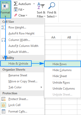
- Go to the Home tab >Cells group, and click the Format button.
- Under Visibility, point to Hide & Unhide, and then select Hide Rows.
Alternatively, you can click Home tab >Format > Row Height… and type 0 in the Row Height box.
Either way, the selected rows will be hidden from view straight away.
In case you don’t want to bother remembering the location of the Hide command on the ribbon, you can access it from the context menu: right click the selected rows, and then click Hide. 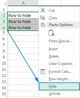
Excel shortcut to hide row
If you’d rather not take your hands off the keyboard, you can quickly hide the selected row(s) by pressing this shortcut: Ctrl + 9
How to unhide rows in Excel
As with hiding rows, Microsoft Excel provides a few different ways to unhide them. Which one to use is a matter of your personal preference. What makes the difference is the area you select to instruct Excel to unhide all hidden rows, only specific rows, or the first row in a sheet.
Unhide rows by using the ribbon
On the Home tab, in the Cells group, click the Format button, point to Hide & Unhide under Visibility, and then click Unhide Rows. 
You select a group of rows including the row above and below the row(s) you want to unhide, right-click the selection, and choose Unhide in the pop-up menu. This method works beautifully for unhiding a single hidden row as well as multiple rows.
For example, to show all hidden rows between rows 1 and 8, select this group of rows like shown in the screenshot below, right-click, and click Unhide: 
Unhide rows with a keyboard shortcut
Here is the Excel Unhide Rows shortcut: Ctrl + Shift + 9
Pressing this key combination (3 keys simultaneously) displays any hidden rows that intersect the selection.
Show hidden rows by double-clicking
In many situations, the fastest way to unhide rows in Excel is to double click them. The beauty of this method is that you don’t need to select anything. Simply hover your mouse over the hidden row headings, and when the mouse pointer turns into a split two-headed arrow, double click. That’s it! 
How to unhide all rows in Excel
In order to unhide all rows on a sheet, you need to select all rows. For this, you can either:
- Click the Select All button (a little triangle at the upper left corner of a sheet, in the intersection of the row and column headings):
- Press the Select All shortcut: Ctrl + A
Please note that in Microsoft Excel, this shortcut behaves differently in different situations. If the cursor is in an empty cell, the whole worksheet is selected. But if the cursor is in one of contiguous cells with data, only that group of cells is selected; to select all cells, press Ctrl+A one more time.
Once the entire sheet is selected, you can unhide all rows by doing one of the following:
- Press Ctrl + Shift + 9 (the fastest way).
- Select Unhide from the right-click menu (the easiest way that does not require remembering anything).
- On the Home tab, click Format >Unhide Rows (the traditional way).
How to unhide all cells in Excel
To unhide all rows and columns, select the whole sheet as explained above, and then press Ctrl + Shift + 9 to show hidden rows and Ctrl + Shift + 0 to show hidden columns.
How to unhide specific rows in Excel
Depending on which rows you want to unhide, select them as described below, and then apply one of the unhide options discussed above.
- To show one or several adjacent rows, select the row above and below the row(s) that you want to unhide.
- To unhide multiple non-adjacent rows, select all the rows between the first and last visible rows in the group.
For example, to unhide rows 3, 7, and 9, you select rows 2 — 10, and then use the ribbon, context menu or keyboard shortcut to unhide them.
How to unhide top rows in Excel
Hiding the first row in Excel is easy, you treat it just like any other row on a sheet. But when one or more top rows are hidden, how do you make them visible again, given that there is nothing above to select?
The clue is to select cell A1. For this, just type A1 in the Name Box, and press Enter. 
Alternatively, go to the Home tab > Editing group, click Find & Select, and then click Go To… . The Go To dialog window pops up, you type A1 in the Reference box, and click OK. 
With cell A1 selected, you can unhide the first hidden row in the usual way, by clicking Format > Unhide Rows on the ribbon, or choosing Unhide from the context menu, or pressing the unhide rows shortcut Ctrl + Shift + 9
Aside from this common approach, there is one more (and faster!) way to unhide first row in Excel. Simply hover over the hidden row heading, and when the mouse pointer turns into a split two-headed arrow, double click: 
Tips and tricks for hiding and unhiding rows in Excel
As you have just seen, hiding and showing rows in Excel is quick and straightforward. In some situations, however, even a simple task can become a challenge. Below you will find easy solutions to a few tricky problems.
How to hide rows containing blank cells
To hide rows that contain any blank cells, proceed with these steps:
- Select the range that contains empty cells you want to hide.
- On the Home tab, in the Editing group, click Find & Select >Go To Special.
- In the Go To Special dialog box, select the Blanks radio button, and click OK. This will select all empty cells in the range.
- Press Ctrl + 9 to hide the corresponding rows.
This method works well when you want to hide all rows that contain at least one blank cell, as shown in the screenshot below: ![]()
If you want to hide blank rows in Excel, i.e. the rows where all cells are blank, then use the COUNTBLANK formula explained in How to remove blank rows to identify such rows.
How to hide rows based on cell value
To hide and show rows based on a cell value in one or more columns, use the capabilities of Excel Filter. It provides a handful of predefined filters for text, numbers and dates as well as an ability to configure a custom filter with your own criteria (please follow the above link for full details).
To unhide filtered rows, you remove filter from a specific column or clear all filters in a sheet, as explained here.
Hide unused rows so that only working area is visible
In situations when you have a small working area on the sheet and a whole lot of unnecessary blank rows and columns, you can hide unused rows in this way:
- Select the row beneath the last row with data (to select the entire row, click on the row header).
- Press Ctrl + Shift + Down arrow to extend the selection to the bottom of the sheet.
- Press Ctrl + 9 to hide the selected rows.
In a similar fashion, you hide unused columns:
- Select an empty column that comes after the last column of data.
- Press Ctrl + Shift + Right arrow to select all other unused columns to the end of the sheet.
- Press Ctrl + 0 to hide the selected columns. Done!
If you decide to unhide all cells later, select the entire sheet, then press Ctrl + Shift + 9 to unhide all rows and Ctrl + Shift + 0 to unhide all columns.
How to locate all hidden rows on a sheet
If your worksheet contains hundreds or thousands of rows, it can be hard to detect hidden ones. The following trick makes the job easy.
- On the Home tab, in the Editing group, click Find & Select >Go To Special. Or press Ctrl+G to open the Go To dialog box, and then click Special.
- In the Go To Special window, select Visible cells only and click OK.

This will select all visible cells and mark the rows adjacent to hidden rows with a white border: 
How to copy visible rows in Excel
Supposing you have hidden a few irrelevant rows, and now you want to copy the relevant data to another sheet or workbook. How would you go about it? Select the visible rows with the mouse and press Ctrl + C to copy them? But that would also copy the hidden rows!
To copy only visible rows in Excel, you’ll have to go about it differently:
- Select visible rows using the mouse.
- Go to the Home tab >Editing group, and click Find & Select >Go To Special.
- In the Go To Special window, select Visible cells only and click OK. That will really select only visible rows like shown in the previous tip.
- Press Ctrl + C to copy the selected rows.
- Press Ctrl + V to paste the visible rows.
Cannot unhide rows in Excel
If you have troubles unhiding rows in your worksheets, it’s most likely because of one of the following reasons.
1. The worksheet is protected
Whenever the Hide and Unhide features are disabled (greyed out) in your Excel, the first thing to check is worksheet protection.
For this, go to the Review tab > Changes group, and see if the Unprotect Sheet button is there (this button appears only in protected worksheets; in an unprotected worksheet, there will be the Protect Sheet button instead). So, if you see the Unprotect Sheet button, click on it.
If you want to keep the worksheet protection but allow hiding and unhiding rows, click the Protect Sheet button on the Review tab, select the Format rows box, and click OK. 
Tip. If the sheet is password-protected, but you cannot remember the password, follow these guidelines to unprotect worksheet without password.
2. Row height is small, but not zero
In case the worksheet is not protected but specific rows still cannot be unhidden, check the height of those rows. The point is that if a row height is set to some small value, between 0.08 and 1, the row seems to be hidden but actually it is not. Such rows cannot be unhidden in the usual way. You have to change the row height to bring them back.
To have it done, perform these steps:
- Select a group of rows, including a row above and a row below the problematic row(s).
- Right click the selection and choose Row Height… from the context menu.
- Type the desired number of the Row Height box (for example the default 15 points) and click OK.
This will make all hidden rows visible again. 
If the row height is set to 0.07 or less, such rows can be unhidden normally, without the above manipulations.
3. Trouble unhiding the first row in Excel
If someone has hidden the first row in a sheet, you may have problems getting it back because you cannot select the row before it. In this case, select cell A1 as explained in How to unhide top rows in Excel and then unhide the row as usual, for example by pressing Ctrl + Shift + 9 .
4. Some rows are filtered out
When the row numbers in your worksheet turn blue, this indicates that some rows are filtered out. To unhide such rows, simply remove all filters on a sheet.
This is how you hide and undie rows in Excel. I thank you for reading and hope to see you on our blog next week!
Источник