
How to Get a Column Number in Excel: Easy Tutorial (2023)
An Excel sheet is two-dimensional – it has rows and columns. By default, row headers in Excel are numbers, and column headers are alphabets.
As the data in your Excel sheet starts to grow in width, the number of columns grows. And this might make it difficult for you to track down a column by its number.
The article below explains different methods of how you can get column numbers in Excel. Also, it focuses on how column numbers might help you in your Excel jobs.
So stay tuned till the end! 😀
Practice the examples shown in the article below by downloading the sample workbook here.
How to get column number with the COLUMN function
If you have never before heard of the COLUMN function, it’s alright. Most Excel users have not.
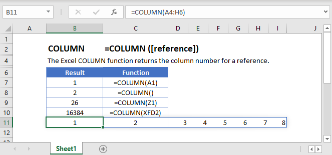
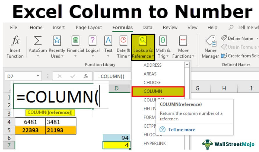
The COLUMN function of Excel is designed to return the number of a column in Excel.
To find the column numbers for different columns in Excel, see the example below.

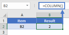
1. Write the COLUMN formula.
=COLUMN()
And this is it!
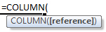
The COLUMN function has just one argument – the reference argument. Interestingly, this argument is also optional.
If omitted, Excel deems it equal to the Cell reference where the formula is written.

We had omitted the argument, so Excel set it equal to Cell B2. Column B comes second in the sequence, so Excel returned ‘2’ as the Column number.
Let’s see this the other way around.
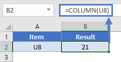
2. Set the reference argument to AAX10.


This time Excel returns column number 726. This means Column AAX is the 726th Column of Excel.
How many columns are there in an Excel Sheet?
The last column of an Excel worksheet is Column XFD. So how many columns are there in a single worksheet?
Let’s do it quickly!
- Press Ctrl + the right arrow button ➡️ to fast forward to the last column of Excel.
- Write the Column formula.
=COLUMN()

16384 Excel Columns to each worksheet.
Let’s double-check the same from Google! 😆

Examples of uses for the COLUMN function
Why would anyone want to use the COLUMN function? The examples below tell why.
Example 1:
The image below shows the grades of a few students (to the left).

To the right side, we want to fetch out the grades for Henry. Easy solution = VLOOKUP.
1. Write the VLOOKUP function as follows.
= VLOOKUP (E1,

The lookup_value is referred to as Cell E1 because it contains the name of the student to look the result for.
2. Refer to the table array where the lookup and the return values are.
= VLOOKUP (E1, A1:B4,

3. For the col_index num argument, nest in the COLUMN function as follows:
= VLOOKUP (F1, A1:B4, COLUMN(B1))
The col_index num argument refers to the column from where the value is to be returned.
And this has to be the number of the column starting from the first column of the table_array.

We want the Grades of Henry to be returned. Grades are listed in column B, so we have referred to Cell B1 (any cell from Column B).

Instead of manually counting the columns, let the COLUMN function do the job.
The VLOOKUP function needs the column number starting from the table array. If the table array starts from any column other than the first column, the above function might not work.
For example, what if the table array above started from Column B and not A?

1. Write the VLOOKUP function as above, and it’d fail to function.
=VLOOKUP (G2, B1:C4, (COLUMN (C1))
It will take the col_index num argument as 3 (Column number of Column C).
Whereas, our table range has only two columns.

2. Deal with such a situation by changing the COLUMN function as follows.
= COLUMN(C1) – COLUMN(A1)
Subtract the number of the column before the table array (Column A) from the return value column (Column C).
3. Rewrite the VLOOKUP function as below.
= VLOOKUP (G1, B1:C4, COLUMN(C1) – COLUMN(A1))
Here are the results!

Example 2:
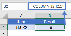
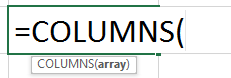
The COLUMN function is not only meant to find the number of a single column. You can also use it to find the number of multiple columns at once.
The data below shows the monthly utility bill of a household.

To find the accumulated utility bill for each month, let’s apply the COLUMN function.
1. Write the COLUMN function as follows.
=COLUMN(A2:F2)

The range A2:F2 tells the number of months for which we need the accumulated bill.

2. Multiply it with the particular cell of the monthly bill.
= H3 * COLUMN(A2:F2)
The cell reference is set to H3 as it contains the monthly bill.


It only takes a single click for Excel to compute the bills for all the months.
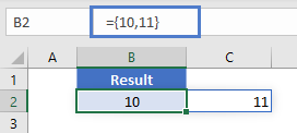
When the reference argument of the column function is defined as a range, the output is an array.
Caution! The SPILL Error:
If the cells of the array are not vacant before the array function operates, Excel gives the #SPILL! Error.

Show column number instead of letter
Only if Excel labeled both the rows and columns with numbers and not alphabets – things would have been much easier!
If you think like that, let’s do it for you.
To change the column letter to numbers in Excel, continue reading.
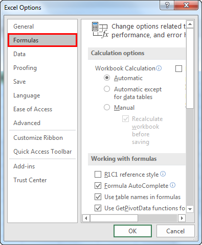
1. Go to File > Options
2. This opens up the Excel options dialog box.

3. Go to Formulas.
4. Under the tab, ‘Working with Formulas’, check the box R1C1 Reference Style.

And swish! Magic. The reference style of columns has changed. 😉

Your Excel worksheet looks all new with a new reference style! Both columns and rows are labeled by numbers.
The R1C1 style reference indicates the Row number and Column number. Accordingly, the cell references will automatically change.
For example, the traditional Cell reference C5 has now become R5C3 (Row number 5 and Column number 3).

This way, you can easily track down the number of columns.
That’s it – Now what?
By now, we have learned to find the column number in Excel through the COLUMN formula, to nest the COLUMN formula in VLOOKUP, and also to change the Column reference style in Excel.
But that’s all about basic Excel. To become an Excel pro you must master the VLOOKUP, SUMIF, and IF functions.
Where can you learn them? Click here to sign up for my free 30-minute email course that will help you master these functions (and more!).
Other relevant resources:
Finding the column number for a specific column or a group of columns can simplify your Excel jobs.
We suggest you also take a quick look into some shortcuts for adding, moving, splitting, clustering, and comparing columns. Once you have learned these shortcuts and tips, you’ll feel no less than an Excel whizz.
Kasper Langmann2023-01-19T12:23:31+00:00
Page load link
Counting is an integral part of data analysis, whether you are tallying the head count of a department in your organization or the number of units that were sold quarter-by-quarter. Excel provides multiple techniques that you can use to count cells, rows, or columns of data. To help you make the best choice, this article provides a comprehensive summary of methods, a downloadable workbook with interactive examples, and links to related topics for further understanding.
Download our examples
You can download an example workbook that gives examples to supplement the information in this article. Most sections in this article will refer to the appropriate worksheet within the example workbook that provides examples and more information.
Download examples to count values in a spreadsheet
In this article
-
Simple counting
-
Use AutoSum
-
Add a Subtotal row
-
Count cells in a list or Excel table column by using the SUBTOTAL function
-
-
Counting based on one or more conditions
-
Video: Use the COUNT, COUNTIF, and COUNTA functions
-
Count cells in a range by using the COUNT function
-
Count cells in a range based on a single condition by using the COUNTIF function
-
Count cells in a column based on single or multiple conditions by using the DCOUNT function
-
Count cells in a range based on multiple conditions by using the COUNTIFS function
-
Count based on criteria by using the COUNT and IF functions together
-
Count how often multiple text or number values occur by using the SUM and IF functions together
-
Count cells in a column or row in a PivotTable
-
-
Counting when your data contains blank values
-
Count nonblank cells in a range by using the COUNTA function
-
Count nonblank cells in a list with specific conditions by using the DCOUNTA function
-
Count blank cells in a contiguous range by using the COUNTBLANK function
-
Count blank cells in a non-contiguous range by using a combination of SUM and IF functions
-
-
Counting unique occurrences of values
-
Count the number of unique values in a list column by using Advanced Filter
-
Count the number of unique values in a range that meet one or more conditions by using IF, SUM, FREQUENCY, MATCH, and LEN functions
-
-
Special cases (count all cells, count words)
-
Count the total number of cells in a range by using ROWS and COLUMNS functions
-
Count words in a range by using a combination of SUM, IF, LEN, TRIM, and SUBSTITUTE functions
-
-
Displaying calculations and counts on the status bar
Simple counting
You can count the number of values in a range or table by using a simple formula, clicking a button, or by using a worksheet function.
Excel can also display the count of the number of selected cells on the Excel status bar. See the video demo that follows for a quick look at using the status bar. Also, see the section Displaying calculations and counts on the status bar for more information. You can refer to the values shown on the status bar when you want a quick glance at your data and don’t have time to enter formulas.
Video: Count cells by using the Excel status bar
Watch the following video to learn how to view count on the status bar.

Use AutoSum
Use AutoSum by selecting a range of cells that contains at least one numeric value. Then on the Formulas tab, click AutoSum > Count Numbers.

Excel returns the count of the numeric values in the range in a cell adjacent to the range you selected. Generally, this result is displayed in a cell to the right for a horizontal range or in a cell below for a vertical range.
Top of Page
Add a Subtotal row
You can add a subtotal row to your Excel data. Click anywhere inside your data, and then click Data > Subtotal.
Note: The Subtotal option will only work on normal Excel data, and not Excel tables, PivotTables, or PivotCharts.

Also, refer to the following articles:
-
Outline (group) data in a worksheet
-
Insert subtotals in a list of data in a worksheet
Top of Page
Count cells in a list or Excel table column by using the SUBTOTAL function
Use the SUBTOTAL function to count the number of values in an Excel table or range of cells. If the table or range contains hidden cells, you can use SUBTOTAL to include or exclude those hidden cells, and this is the biggest difference between SUM and SUBTOTAL functions.
The SUBTOTAL syntax goes like this:
SUBTOTAL(function_num,ref1,[ref2],…)

To include hidden values in your range, you should set the function_num argument to 2.
To exclude hidden values in your range, set the function_num argument to 102.
Top of Page
Counting based on one or more conditions
You can count the number of cells in a range that meet conditions (also known as criteria) that you specify by using a number of worksheet functions.
Video: Use the COUNT, COUNTIF, and COUNTA functions
Watch the following video to see how to use the COUNT function and how to use the COUNTIF and COUNTA functions to count only the cells that meet conditions you specify.
Top of Page
Count cells in a range by using the COUNT function
Use the COUNT function in a formula to count the number of numeric values in a range.

In the above example, A2, A3, and A6 are the only cells that contains numeric values in the range, hence the output is 3.
Note: A7 is a time value, but it contains text (a.m.), hence COUNT does not consider it a numerical value. If you were to remove a.m. from the cell, COUNT will consider A7 as a numerical value, and change the output to 4.
Top of Page
Count cells in a range based on a single condition by using the COUNTIF function
Use the COUNTIF function function to count how many times a particular value appears in a range of cells.

Top of Page
Count cells in a column based on single or multiple conditions by using the DCOUNT function
DCOUNT function counts the cells that contain numbers in a field (column) of records in a list or database that match conditions that you specify.
In the following example, you want to find the count of the months including or later than March 2016 that had more than 400 units sold. The first table in the worksheet, from A1 to B7, contains the sales data.

DCOUNT uses conditions to determine where the values should be returned from. Conditions are typically entered in cells in the worksheet itself, and you then refer to these cells in the criteria argument. In this example, cells A10 and B10 contain two conditions—one that specifies that the return value must be greater than 400, and the other that specifies that the ending month should be equal to or greater than March 31st, 2016.
You should use the following syntax:
=DCOUNT(A1:B7,»Month ending»,A9:B10)
DCOUNT checks the data in the range A1 through B7, applies the conditions specified in A10 and B10, and returns 2, the total number of rows that satisfy both conditions (rows 5 and 7).
Top of Page
Count cells in a range based on multiple conditions by using the COUNTIFS function
The COUNTIFS function is similar to the COUNTIF function with one important exception: COUNTIFS lets you apply criteria to cells across multiple ranges and counts the number of times all criteria are met. You can use up to 127 range/criteria pairs with COUNTIFS.
The syntax for COUNTIFS is:
COUNTIFS(criteria_range1, criteria1, [criteria_range2, criteria2],…)
See the following example:

Top of Page
Count based on criteria by using the COUNT and IF functions together
Let’s say you need to determine how many salespeople sold a particular item in a certain region or you want to know how many sales over a certain value were made by a particular salesperson. You can use the IF and COUNT functions together; that is, you first use the IF function to test a condition and then, only if the result of the IF function is True, you use the COUNT function to count cells.
Notes:
-
The formulas in this example must be entered as array formulas. If you have opened this workbook in Excel for Windows or Excel 2016 for Mac and want to change the formula or create a similar formula, press F2, and then press Ctrl+Shift+Enter to make the formula return the results you expect. In earlier versions of Excel for Mac, use
 +Shift+Enter.
 -
For the example formulas to work, the second argument for the IF function must be a number.

Top of Page
Count how often multiple text or number values occur by using the SUM and IF functions together
In the examples that follow, we use the IF and SUM functions together. The IF function first tests the values in some cells and then, if the result of the test is True, SUM totals those values that pass the test.
Example 1

The above function says if C2:C7 contains the values Buchanan and Dodsworth, then the SUM function should display the sum of records where the condition is met. The formula finds three records for Buchanan and one for Dodsworth in the given range, and displays 4.
Example 2

The above function says if D2:D7 contains values lesser than $9000 or greater than $19,000, then SUM should display the sum of all those records where the condition is met. The formula finds two records D3 and D5 with values lesser than $9000, and then D4 and D6 with values greater than $19,000, and displays 4.
Example 3

The above function says if D2:D7 has invoices for Buchanan for less than $9000, then SUM should display the sum of records where the condition is met. The formula finds that C6 meets the condition, and displays 1.
Important: The formulas in this example must be entered as array formulas. That means you press F2 and then press Ctrl+Shift+Enter. In earlier versions of Excel for Mac use  +Shift+Enter.
See the following Knowledge Base articles for additional tips:
-
XL: Using SUM(IF()) As an Array Function Instead of COUNTIF() with AND
-
XL: How to Count the Occurrences of a Number or Text in a Range
Top of Page
Count cells in a column or row in a PivotTable
A PivotTable summarizes your data and helps you analyze and drill down into your data by letting you choose the categories on which you want to view your data.
You can quickly create a PivotTable by selecting a cell in a range of data or Excel table and then, on the Insert tab, in the Tables group, clicking PivotTable.

Let’s look at a sample scenario of a Sales spreadsheet, where you can count how many sales values are there for Golf and Tennis for specific quarters.
Note: For an interactive experience, you can run these steps on the sample data provided in the PivotTable sheet in the downloadable workbook.
-
Enter the following data in an Excel spreadsheet.
-
Select A2:C8
-
Click Insert > PivotTable.
-
In the Create PivotTable dialog box, click Select a table or range, then click New Worksheet, and then click OK.
An empty PivotTable is created in a new sheet.
-
In the PivotTable Fields pane, do the following:
-
Drag Sport to the Rows area.
-
Drag Quarter to the Columns area.
-
Drag Sales to the Values area.
-
Repeat step c.
The field name displays as SumofSales2 in both the PivotTable and the Values area.
At this point, the PivotTable Fields pane looks like this:
-
In the Values area, click the dropdown next to SumofSales2 and select Value Field Settings.
-
In the Value Field Settings dialog box, do the following:
-
In the Summarize value field by section, select Count.
-
In the Custom Name field, modify the name to Count.
-
Click OK.
-
The PivotTable displays the count of records for Golf and Tennis in Quarter 3 and Quarter 4, along with the sales figures.
-


Top of Page
Counting when your data contains blank values
You can count cells that either contain data or are blank by using worksheet functions.
Count nonblank cells in a range by using the COUNTA function
Use the COUNTA function function to count only cells in a range that contain values.
When you count cells, sometimes you want to ignore any blank cells because only cells with values are meaningful to you. For example, you want to count the total number of salespeople who made a sale (column D).

COUNTA ignores the blank values in D3, D4, D8, and D11, and counts only the cells containing values in column D. The function finds six cells in column D containing values and displays 6 as the output.
Top of Page
Count nonblank cells in a list with specific conditions by using the DCOUNTA function
Use the DCOUNTA function to count nonblank cells in a column of records in a list or database that match conditions that you specify.
The following example uses the DCOUNTA function to count the number of records in the database that is contained in the range A1:B7 that meet the conditions specified in the criteria range A9:B10. Those conditions are that the Product ID value must be greater than or equal to 2000 and the Ratings value must be greater than or equal to 50.

DCOUNTA finds two rows that meet the conditions- rows 2 and 4, and displays the value 2 as the output.
Top of Page
Count blank cells in a contiguous range by using the COUNTBLANK function
Use the COUNTBLANK function function to return the number of blank cells in a contiguous range (cells are contiguous if they are all connected in an unbroken sequence). If a cell contains a formula that returns empty text («»), that cell is counted.
When you count cells, there may be times when you want to include blank cells because they are meaningful to you. In the following example of a grocery sales spreadsheet. suppose you want to find out how many cells don’t have the sales figures mentioned.

Note: The COUNTBLANK worksheet function provides the most convenient method for determining the number of blank cells in a range, but it doesn’t work very well when the cells of interest are in a closed workbook or when they do not form a contiguous range. The Knowledge Base article XL: When to Use SUM(IF()) instead of CountBlank() shows you how to use a SUM(IF()) array formula in those cases.
Top of Page
Count blank cells in a non-contiguous range by using a combination of SUM and IF functions
Use a combination of the SUM function and the IF function. In general, you do this by using the IF function in an array formula to determine whether each referenced cell contains a value, and then summing the number of FALSE values returned by the formula.
See a few examples of SUM and IF function combinations in an earlier section Count how often multiple text or number values occur by using the SUM and IF functions together in this topic.
Top of Page
Counting unique occurrences of values
You can count unique values in a range by using a PivotTable, COUNTIF function, SUM and IF functions together, or the Advanced Filter dialog box.
Count the number of unique values in a list column by using Advanced Filter
Use the Advanced Filter dialog box to find the unique values in a column of data. You can either filter the values in place or you can extract and paste them to a new location. Then you can use the ROWS function to count the number of items in the new range.
To use Advanced Filter, click the Data tab, and in the Sort & Filter group, click Advanced.
The following figure shows how you use the Advanced Filter to copy only the unique records to a new location on the worksheet.

In the following figure, column E contains the values that were copied from the range in column D.

Notes:
-
If you filter your data in place, values are not deleted from your worksheet — one or more rows might be hidden. Click Clear in the Sort & Filter group on the Data tab to display those values again.
-
If you only want to see the number of unique values at a quick glance, select the data after you have used the Advanced Filter (either the filtered or the copied data) and then look at the status bar. The Count value on the status bar should equal the number of unique values.
For more information, see Filter by using advanced criteria
Top of Page
Count the number of unique values in a range that meet one or more conditions by using IF, SUM, FREQUENCY, MATCH, and LEN functions
Use various combinations of the IF, SUM, FREQUENCY, MATCH, and LEN functions.
For more information and examples, see the section «Count the number of unique values by using functions» in the article Count unique values among duplicates.
Top of Page
Special cases (count all cells, count words)
You can count the number of cells or the number of words in a range by using various combinations of worksheet functions.
Count the total number of cells in a range by using ROWS and COLUMNS functions
Suppose you want to determine the size of a large worksheet to decide whether to use manual or automatic calculation in your workbook. To count all the cells in a range, use a formula that multiplies the return values using the ROWS and COLUMNS functions. See the following image for an example:

Top of Page
Count words in a range by using a combination of SUM, IF, LEN, TRIM, and SUBSTITUTE functions
You can use a combination of the SUM, IF, LEN, TRIM, and SUBSTITUTE functions in an array formula. The following example shows the result of using a nested formula to find the number of words in a range of 7 cells (3 of which are empty). Some of the cells contain leading or trailing spaces — the TRIM and SUBSTITUTE functions remove these extra spaces before any counting occurs. See the following example:

Now, for the above formula to work correctly, you have to make this an array formula, otherwise the formula returns the #VALUE! error. To do that, click on the cell that has the formula, and then in the Formula bar, press Ctrl + Shift + Enter. Excel adds a curly bracket at the beginning and the end of the formula, thus making it an array formula.
For more information on array formulas, see Overview of formulas in Excel and Create an array formula.
Top of Page
Displaying calculations and counts on the status bar
When one or more cells are selected, information about the data in those cells is displayed on the Excel status bar. For example, if four cells on your worksheet are selected, and they contain the values 2, 3, a text string (such as «cloud»), and 4, all of the following values can be displayed on the status bar at the same time: Average, Count, Numerical Count, Min, Max, and Sum. Right-click the status bar to show or hide any or all of these values. These values are shown in the illustration that follows.

Top of Page
Need more help?
You can always ask an expert in the Excel Tech Community or get support in the Answers community.
Содержание
- Columns and rows are labeled numerically in Excel
- Symptoms
- Cause
- Resolution
- More information
- A1 Reference Style vs. R1C1 Reference Style
- The A1 Reference Style
- The R1C1 Reference Style
- References
- Automatically number rows
- What do you want to do?
- Fill a column with a series of numbers
- Use the ROW function to number rows
- Display or hide the fill handle
- COLUMN Function Examples – Excel & Google Sheets
- COLUMN Function Overview
- COLUMN function Syntax and inputs:
- COLUMN Function – Single Cell
- COLUMN Function with no Reference
- COLUMN Function with a Range
- Excel 2019 or older
- Excel 365
- COLUMN Function in Google Sheets
- Additional Notes
- COLUMN Function
- Related functions
- Summary
- Purpose
- Return value
- Arguments
- Syntax
- Usage notes
- Examples
- Excel Column to Number
- Column Letter to Number in Excel
- How to Find Column Numbers in Excel? (with Examples)
- Example #1
- Example #2
- Example #3
- Example #4
- Things to Remember
- Recommended Articles
Columns and rows are labeled numerically in Excel
Symptoms
Your column labels are numeric rather than alphabetic. For example, instead of seeing A, B, and C at the top of your worksheet columns, you see 1, 2, 3, and so on.
Cause
This behavior occurs when the R1C1 reference style check box is selected in the Options dialog box.
Resolution
To change this behavior, follow these steps:
- Start Microsoft Excel.
- On the Tools menu, click Options.
- Click the Formulas tab.
- Under Working with formulas, click to clear the R1C1 reference style check box (upper-left corner), and then click OK.
If you select the R1C1 reference style check box, Excel changes the reference style of both row and column headings, and cell references from the A1 style to the R1C1 style.
More information
A1 Reference Style vs. R1C1 Reference Style
The A1 Reference Style
By default, Excel uses the A1 reference style, which refers to columns as letters (A through IV, for a total of 256 columns), and refers to rows as numbers (1 through 65,536). These letters and numbers are called row and column headings. To refer to a cell, type the column letter followed by the row number. For example, D50 refers to the cell at the intersection of column D and row 50. To refer to a range of cells, type the reference for the cell that is in the upper-left corner of the range, type a colon (:), and then type the reference to the cell that is in the lower-right corner of the range.
The R1C1 Reference Style
Excel can also use the R1C1 reference style, in which both the rows and the columns on the worksheet are numbered. The R1C1 reference style is useful if you want to compute row and column positions in macros. In the R1C1 style, Excel indicates the location of a cell with an «R» followed by a row number and a «C» followed by a column number.
References
For more information about this topic, click Microsoft Excel Help on the Help menu, type about cell and range references in the Office Assistant or the Answer Wizard, and then click Search to view the topic.
Источник
Automatically number rows
Unlike other Microsoft 365 programs, Excel does not provide a button to number data automatically. But, you can easily add sequential numbers to rows of data by dragging the fill handle to fill a column with a series of numbers or by using the ROW function.
Tip: If you are looking for a more advanced auto-numbering system for your data, and Access is installed on your computer, you can import the Excel data to an Access database. In an Access database, you can create a field that automatically generates a unique number when you enter a new record in a table.
What do you want to do?
Fill a column with a series of numbers
Select the first cell in the range that you want to fill.
Type the starting value for the series.
Type a value in the next cell to establish a pattern.
Tip: For example, if you want the series 1, 2, 3, 4, 5. type 1 and 2 in the first two cells. If you want the series 2, 4, 6, 8. type 2 and 4.
Select the cells that contain the starting values.
Note: In Excel 2013 and later, the Quick Analysis button is displayed by default when you select more than one cell containing data. You can ignore the button to complete this procedure.
Drag the fill handle  across the range that you want to fill.
Note: As you drag the fill handle across each cell, Excel displays a preview of the value. If you want a different pattern, drag the fill handle by holding down the right-click button, and then choose a pattern.
To fill in increasing order, drag down or to the right. To fill in decreasing order, drag up or to the left.
Tip: If you do not see the fill handle, you may have to display it first. For more information, see Display or hide the fill handle.
Note: These numbers are not automatically updated when you add, move, or remove rows. You can manually update the sequential numbering by selecting two numbers that are in the right sequence, and then dragging the fill handle to the end of the numbered range.
Use the ROW function to number rows
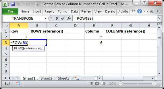
In the first cell of the range that you want to number, type =ROW(A1).
The ROW function returns the number of the row that you reference. For example, =ROW(A1) returns the number 1.
Drag the fill handle across the range that you want to fill.
Tip: If you do not see the fill handle, you may have to display it first. For more information, see Display or hide the fill handle.
These numbers are updated when you sort them with your data. The sequence may be interrupted if you add, move, or delete rows. You can manually update the numbering by selecting two numbers that are in the right sequence, and then dragging the fill handle to the end of the numbered range.
If you are using the ROW function, and you want the numbers to be inserted automatically as you add new rows of data, turn that range of data into an Excel table. All rows that are added at the end of the table are numbered in sequence. For more information, see Create or delete an Excel table in a worksheet.
To enter specific sequential number codes, such as purchase order numbers, you can use the ROW function together with the TEXT function. For example, to start a numbered list by using 000-001, you enter the formula =TEXT(ROW(A1),»000-000″) in the first cell of the range that you want to number, and then drag the fill handle to the end of the range.
Display or hide the fill handle
The fill handle displays by default, but you can turn it on or off.
In Excel 2010 and later, click the File tab, and then click Options.
In Excel 2007, click the Microsoft Office Button  , and then click Excel Options.
In the Advanced category, under Editing options, select or clear the Enable fill handle and cell drag-and-drop check box to display or hide the fill handle.
Note: To help prevent replacing existing data when you drag the fill handle, ensure the Alert before overwriting cells check box is selected. If you do not want Excel to display a message about overwriting cells, you can clear this check box.
Источник
COLUMN Function Examples – Excel & Google Sheets
Download the example workbook
This Tutorial demonstrates how to use the Excel COLUMN Function in Excel to look up the column number.
COLUMN Function Overview
The COLUMN Function Returns the column number of a cell reference.
To use the COLUMN Excel Worksheet Function, select a cell and type:
(Notice how the formula inputs appear)
COLUMN function Syntax and inputs:
reference – Cell reference that you want to determine the column # of.
COLUMN Function – Single Cell
The COLUMN Function returns the column number of the given cell reference.
COLUMN Function with no Reference
If no cell reference is provided, the COLUMN Function will return the column number where the formula is entered
COLUMN Function with a Range
You can also input entire ranges of cells into the COLUMN Function. When doing so, the COLUMN Function behaves differently in Excel 2019 (or earlier) vs. Excel 365 or newer version of Excel.
Excel 2019 or older
In previous versions of Excel, the COLUMN Function returns an array containing the column values of all the cells in the range, but only displays the first result in the cell.
If you click the cell containing the formula and press F9, all the results are displayed in curly brackets as an array.
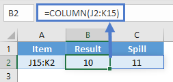
Excel 365
However, Excel 365 (and newer versions of Excel, presumably) comes with a spill range feature. Here, the COLUMN Function will return the columns of all cells in the range, “spilled” into the next cells.
COLUMN Function in Google Sheets
The COLUMN Function works exactly the same in Google Sheets as in Excel:
Additional Notes
Use the COLUMN Function to return the column number of a cell reference. What if you want the column letter of a cell reference? Use this complicated formula instead:
This formula calculates the column number with the COLUMN Function and calculates the address of a cell in row 1 of that column using the ADDRESS Function. Then it uses the SUBSTITUTE Function to remove the row number (1), so all that remains is the column letter.
Источник
COLUMN Function

Summary
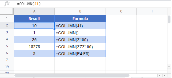
The Excel COLUMN function returns the column number for a reference. For example, COLUMN(C5) returns 3, since C is the third column in the spreadsheet. When no reference is provided, COLUMN returns the column number of the cell which contains the formula.
Purpose
Return value
Arguments
- reference — [optional] A reference to a cell or range of cells.
Syntax
Usage notes
The COLUMN function returns the column number of a reference. For example, COLUMN(C5) returns 3, since C is the third column in the spreadsheet. COLUMN takes just one argument, called reference, which can be empty, a cell reference, or a range. When no reference is provided, COLUMN returns the column number of the cell which contains the formula.
Examples
With a single cell reference, COLUMN returns the associated column number:
When a reference is not provided, COLUMN returns the column number of the cell the formula resides in. For example, if the following formula is entered in cell D6, the result is 4:
When COLUMN is given a range, it returns the column numbers for that range:
In Excel 365, which supports dynamic array formulas, the result is an array <5,6,7>that spills horizontally into three cells, starting with the cell the formula resides in. In earlier Excel versions, the first item of the array (5) will display in one cell only.
To get Excel 365 to return a single value, you can use the implicit intersection operator (@):
This @ symbol disables array behavior and tells Excel you want a single value.
Источник
Excel Column to Number


Column Letter to Number in Excel
Figuring out which row you are in is as easy as you like. But, how do you tell which column you are in now? Excel has 16,384 columns, represented by alphabetic characters in Excel. So, suppose you want to find the column CP. How do you tell?
Yes, it is almost impossible to figure out the column number in Excel. However, nothing to worry about because we have a built-in function called COLUMN in excel COLUMN In Excel Column function finds out the column numbers of the target cells in excel. It takes one argument which is the target cell as reference. Note that this function does not give the value of the cell as it returns only the column number of the cell. read more , which can tell the exact column number we are in right now or find the column number of the supplied argument.
Table of contents
You are free to use this image on your website, templates, etc., Please provide us with an attribution link How to Provide Attribution? Article Link to be Hyperlinked
For eg:
Source: Excel Column to Number (wallstreetmojo.com)
How to Find Column Numbers in Excel? (with Examples)
Example #1
We can get the current column number by using the COLUMN function in Excel.
- We have opened a new workbook and typed some of the values in the worksheet.

Let us say we are in cell D7, and we want to know the column number of this cell.

To find the current column number, we must write the COLUMN function in the Excel cell and do not pass any argument; close the bracket.

Press the “Enter” key. As a result, we will have a current column number in Excel.

Example #2
We can get the column number of the different cells by using the COLUMN function in Excel.
Getting the current column is not the toughest task at all. Suppose we want to know the column number of the cell CP5 and how we get that column number.
- We can write the COLUMN function and pass the specified cell value in any cells.

- Then press the “Enter” key. It will return the column number of CP5.

We have applied the COLUMN formula in cell D6 and passed the argument as CP5, i.e., cell reference Cell Reference Cell reference in excel is referring the other cells to a cell to use its values or properties. For instance, if we have data in cell A2 and want to use that in cell A1, use =A2 in cell A1, and this will copy the A2 value in A1. read more of CP5 cell. However, unlike normal cell reference, it will not return the value in the cell CP5. Rather, it will return the column number of CP5.
So, the column number of the cell CP5 is 94.
Example #3
We can get how many columns are selected in the range by using the COLUMNS function in Excel.
We have learned how to get the current cell column number and specified cell column number in Excel. But, how do you tell how many columns are selected in the range?
Assume we want to know how many columns are from the range C5 to N5.
- We can open the formula COLUMNS in any cell and select the range as C5 toN5.

- Press the “Enter” key to get the desired result.
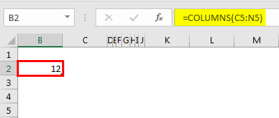
So totally, we have selected 12 columns in the range C5 to N5.
In this way, by using the COLUMN and COLUMNS function in Excel, we can get the two different kinds of results, which can help us calculate or identify the exact column when dealing with huge datasets.
Example #4
We can change the cell reference form to R1C1 references in Excel.
By default, we have cell references, all the rows are represented numerically, and all the columns are represented alphabetically.

It is the usual spreadsheet structure we are familiar with. The cell reference is started with the column alphabet and then followed by row numbers.
As we learned earlier in the article, we need to use the COLUMN function to get the column number. How about changing the column headers from the alphabet to numbers like our row headers? Like the image below.

It is called ROW-COLUMN reference in Excel. Now, take a look at the below image and the reference type.
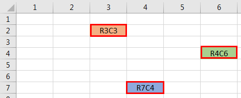
Unlike our standard cell reference, reference starts with a row number followed by a column number, not an alphabet.
Follow the below steps to change it to the R1C1 reference style.
- We must first go to the “File” and “Options.”

- Next, go to “Formulas” under “Options.”
- Working with “Formulas,” select the checkbox “R1C1 reference style” and click “OK.”

Once we click “OK,” cells will change to R1C1 references.
Things to Remember
- The R1C1 cell reference is the rarely followed cell reference in Excel. As a result, we may get confused easily at the start.
- We see column alphabet first and row number next in normal cell references. But in R1C1 cell references, the row number will come first and the column number.
- The COLUMN function can return the current column number and the supplied column number.
- The R1C1 cell reference makes it easy to find the column number easily.
Recommended Articles
This article has been a guide to Column Letter to Numbers in Excel. We discuss finding column numbers in Excel using the COLUMN and COLUMNS functions. You may learn more about Excel from the following articles: –
Источник
How to get the row or column number of the current cell or any other cell in Excel.
This tutorial covers important functions that allow you to do everything from alternate row and column shading to incrementing values at specified intervals and much more.
We will use the ROW and COLUMN function for this. Here is an example of the output from these functions.
Though this doesn’t look like much, these functions allow for the creation of powerful formulas when combined with other functions. Now, let’s look at how to create them.
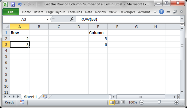
Get a Cell’s Row Number
Syntax
This function returns the number of the row that a particular cell is in.
If you leave the function empty, it will return the row number for the current cell in which this function has been placed.
If you put a cell reference within this function, it will return the row number for that cell reference.
This example would return 1 since cell A1 is in row 1. If it was =ROW(C24) the function would return the number 24 because cell C24 is in row 24.
Examples
Now that you know how this function works, it may seem rather useless. Here are links to two examples where this function is key.
Increment a Value Every X Number of Rows in Excel
Shade Every Other Row in Excel Quickly
Get a Cell’s Column Number
Syntax
This function returns the number of the column that a particular cell is in. It counts from left to right, where A is 1 and B is 2 and so on.
If you leave the function empty, it will return the column number for the current cell in which this function has been placed.
If you put a cell reference within this function, it will return the column number for that cell reference.
This example would return 1 since cell A1 is in row 1. If it was =COLUMN (C24) the function would return the number 3 because cell C24 is in column number 3.
Examples
The COLUMN function works just like the ROW function does except that it works on columns, going left to right, whereas the ROW function works on rows, going up and down.
As such, almost every example where ROW is used could be converted to use COLUMN based on your needs.
Notes
The ROW and COLUMN functions are building blocks in that they help you create more complex formulas in Excel. Alone, these functions are pretty much worthless, but, if you can memorize them and keep them for later, you will start to find more and more uses for them when working in large data sets. The examples provided above in the ROW section cover only two of many different ways you can use these functions to create more powerful and helpful spreadsheets.
Similar Content on TeachExcel
Sum Values from Every X Number of Rows in Excel
Tutorial: Add values from every x number of rows in Excel. For instance, add together every other va…
Formulas to Remove First or Last Character from a Cell in Excel
Tutorial: Formulas that allow you to quickly and easily remove the first or last character from a ce…
Formula to Delete the First or Last Word from a Cell in Excel
Tutorial:
Excel formula to delete the first or last word from a cell.
You can copy and paste the fo…
Reverse the Contents of a Cell in Excel — UDF
Macro: Reverse cell contents with this free Excel UDF (user defined function). This will mir…
Excel Function to Remove All Text OR All Numbers from a Cell
Tutorial: How to create and use a function that removes all text or all numbers from a cell, whichev…
Get the First Word from a Cell in Excel
Tutorial: How to use a formula to get the first word from a cell in Excel. This works for a single c…