A cell reference or cell address is a combination of a column letter and a row number that identifies a cell on a worksheet. For example, A1 refers to the cell at the intersection of column A and row 1; B2 refers to the second cell in column B, and so on.
Contents
- 1 What is the function of cell address?
- 2 What is the cell address in a formula called?
- 3 What is the cell address of the first cell in Excel?
- 4 What is cell address give example?
- 5 What is a cell reference?
- 6 What are the three types of cell references in Excel?
- 7 How do you reference a cell reference in Excel?
- 8 What is the cell address of the last cell in a worksheet?
- 9 Is the address of column 27 and 30?
- 10 What is the first and last cell address in Excel?
- 11 What is cell address explain its types?
- 12 What is the difference between cell and cell address?
- 13 What is a cell reference class 9?
- 14 What is cell referencing Class 7?
- 15 What is cell and cell reference?
- 16 What is address example?
- 17 How is an address formatted?
- 18 What is referencing and its types?
- 19 What is B $3 in Excel?
- 20 What are Excel cell references by default?
What is the function of cell address?
The ADDRESS function returns the address for a cell based on a given row and column number. For example, =ADDRESS(1,1) returns $A$1. ADDRESS can return a relative, mixed, or absolute reference, and can be used to construct a cell reference inside a formula.
What is the cell address in a formula called?
cell reference
Answer. The cell address in a formula is also called cell reference.
What is the cell address of the first cell in Excel?
=ADDRESS(1,1) – returns the address of the first cell (i.e. the cell at the intersection of the first row and first column) as an absolute cell reference $A$1. =ADDRESS(1,1,4) – returns the address of the first cell as a relative cell reference A1.
What is cell address give example?
A reference is a cell’s address. It identifies a cell or range of cells by referring to the column letter and row number of the cell(s). For example, A1 refers to the cell at the intersection of column A and row 1. The reference tells Formula One for Java to use the contents of the referenced cell(s) in the formula.
What is a cell reference?
A cell reference refers to a cell or a range of cells on a worksheet and can be used in a formula so that Microsoft Office Excel can find the values or data that you want that formula to calculate.
What are the three types of cell references in Excel?
Relative, Absolute and Mixed
A key element of a formula is the cell reference, and there are three types: Relative. Absolute. Mixed.
How do you reference a cell reference in Excel?
Use cell references in a formula
- Click the cell in which you want to enter the formula.
- In the formula bar. , type = (equal sign).
- Do one of the following, select the cell that contains the value you want or type its cell reference.
- Press Enter.
What is the cell address of the last cell in a worksheet?
Answer: The intersection of row 1048576 and column XFD is called XFD1048576.
Is the address of column 27 and 30?
So, it will be called AA33.
What is the first and last cell address in Excel?
Answer: =ADDRESS(1,1) – returns the address of the first cell (i.e. the cell at the intersection of the first row and first column) as an absolute cell reference $A$1. =ADDRESS(1,1,4) – returns the address of the first cell as a relative cell reference A1.
What is cell address explain its types?
There are two types of cell references: relative and absolute. Relative and absolute references behave differently when copied and filled to other cells. Relative references change when a formula is copied to another cell. Absolute references, on the other hand, remain constant no matter where they are copied.
What is the difference between cell and cell address?
A cell is a single box in the excel spreadsheet which has only one row and one column address. In Excel, the rows are listed as numbers and the columns are named as letters.For example, if we select a 3×3 area in excel starting from the cell B2, the address of the cell range will be shown as B2:D4.
What is a cell reference class 9?
Cell Reference
A reference identifies a cell or a range of cells on a worksheet and tells MS Excel where to look for value or data to be used in a formula. Using reference, we can use data present in different parts of a worksheet or on a different worksheet or another workbook.
What is cell referencing Class 7?
Cell referencing helps us to identify the behaviour of a cell address in a formula when it is copied from one to another cell. The three types of the referencing are: i. RELATIVE REFERENCING: In this type of referencing both parts of the cell address are not fixed. For example: B3*C3.
What is cell and cell reference?
A cell reference in Excel refers to the value of a different cell or cell range on the current worksheet or a different worksheet within the spreadsheet. A cell reference can be used as a variable in a formula.
What is address example?
Frequency: The definition of an address is a written or verbal statement, or the physical location of something. An example of an address is the President’s Inaugural speech. 123 Main Street, New York, NY 10030 is an example of an address.
How is an address formatted?
The name of the sender should be placed on the first line. If you’re sending from a business, you would list the company name on the next line. Next, you should write out the building number and street name. The final line should have the city, state and ZIP code for the address.
What is referencing and its types?
Explanation:
- Relative referencing : In relative referencing, both column part and row part are not fixed .
- Absolute referencing : In absolute referencing, both column part and row part are fixed.
- Mixed referencing : In mixed referencing,either column part or row part is fixed.
Otherwise, it does change. That is, the $ sign “anchors” a row number or column letter when you copy it.
How to Use Absolute and Relative Cell References in Excel Formulas.
| =B3 | tap {F4} to get: |
|---|---|
| =B$3 | tap {F4} to get: |
| =$B3 | tap {F4} to get: |
| =B3 | (etc) |
What are Excel cell references by default?
By default, a cell reference is a relative reference, which means that the reference is relative to the location of the cell. If, for example, you refer to cell A2 from cell C2, you are actually referring to a cell that is two columns to the left (C minus A)—in the same row (2).
How to Get Cell Address in Excel (ADDRESS + CELL functions)
To obtain information about any cell in Excel, we have two functions: the CELL and the ADDRESS function.
Using these functions, you can get the address, the reference, the formula, the formatting (and much more) of a cell.
These are some of Excel’s most underrated functions, and it’s about time you learn why🤷♂️
So jump right into the guide below. And don’t forget to download our free sample workbook here as you scroll down.
How to use the ADDRESS function
The Excel ADDRESS function returns the cell address for a given row number and column letter.
It has a large but simple syntax that reads as follows:
=ADDRESS(row_num, column_num, [abs_num], [a1], [sheet_text])
In order to address the first cell (Cell A1):
- Write the ADDRESS function as follows:
=ADDRESS(1,1)
- Hit Enter to reach the following result.

The first argument represents the row number (Row 1). The second argument represents the column number (Column 1). And so the resulting ADDRESS is $A$1.
That’s all that you need – the rest of the arguments are only optional ✌
- Now write the ADDRESS function with the third argument (abs_num) set to 4.
=ADDRESS(1,1,4)
- Press Enter and here are the results:

By adding 4 as the [abs_num] argument, Excel changes our result to a relative cell reference. Something completely different from what we saw earlier.
That’s because different values for the abs_num argument return different address types.
Pro Tip!
For the [abs_num] argument:
- If you enter 1, the address type will be an absolute cell reference ($A$1).
- If you enter 2, the address type will be a mixed cell reference. (A$1 – An absolute row reference, and a relative column reference).
- If you enter 3, the address type will be a mixed cell reference. ($A1 – An absolute column reference, and a relative row reference).
- If you enter 4, the address type will be a relative cell reference (A1).
In the first example, we omitted the abs_num argument and Excel set it to 1 by default. The result was, therefore, an absolute cell reference.
But the formula doesn’t just stop here🚀
- Include the fourth argument [a1] to modify this formula further.
=ADDRESS(1,1,4,0)

Here, 0 represents the reference style.
Note that the result is in a different style from our previous example. That’s because we opted for the R1C1 reference style in which columns and rows are represented by numbers.
- To get the result in A1 reference style, add 1 as the [a1] argument :
=ADDRESS(1,1,4,1)

Note that we got the same result for our second example too.
That’s because if we omit the [a1] argument, Excel, by default, sets it to 1.
And what if you want the cell address from a different Excel sheet than the one you are currently on?
For this, you need to use the last optional argument of the ADDRESS function, i.e., [sheet_text].
It identifies the worksheet you want the cell address for 👀 Let’s try it out here:
- Write the [sheet_text] argument of the ADDRESS function as below:
=ADDRESS(1,1,4,1,”Sheet1″)

With the sheet_text argument as above, Excel generates an external reference. It returns the name of the worksheet with the cell address.
Like in the above example, Excel returns the address of the cell from Sheet 1. The Cell address is therefore prefixed by the worksheet name “Sheet1”.
If this argument is omitted, the resulting cell address won’t contain the worksheet name. And the address of the cell will be of the current sheet, by default.
How to use the CELL function
Until now we’ve seen how the ADDRESS function helps you find the address of a cell in Excel.
But what if you want to know about the location, format, formula, and content of a cell too🤔
The CELL function of Excel will help you fetch all these (and even other details about a cell). The syntax of this function reads as follows:
=CELL(info_type, [reference])
Starting with info_type, write the CELL function like this:
=CELL (
As you start writing the CELL function, Excel launches a drop-down menu of options for the argument “info_type“.

You can select from any of the 12 options in the drop-down menu above.
For example, select the option “Address” as the info_type argument. And Excel would return the address of the active (or the referred) cell.
= CELL (“Address”)

Note that we omitted the second argument of the CELL Function in the above example, i.e., [reference].
And so, the function returned the address of the active cell (Cell A2).
Pro Tip!
As the reference argument, you can refer to a single or a range of cells.
That’s not it – we still have 11 more info types to try and test.
So let’s change the arguments of our function as follows:
=CELL (“col”, A3)
Note that here we have created a reference to Cell A3 as the [reference] argument.

In this example, “col” represents the column number of cell A3 (the referred cell). The result given by Excel is 1 (the Column number for Cell A3).
Similarly, you can try different info_types to get different information about a cell. Like the following:
=CELL (“type”, A4)

“Type” returns the type of the referred cell.
Excel returned the value “B” indicating that the cell is blank. This is because we have referred to Cell A4 which is an empty string.
Pro Tip!
Under the “type” mode, if your cell contains a text constant, the result will be “I“. “B” if the cell is blank and “V” if the cell has any other data type.
The CELL function offers a wide variety of info types that you might fetch for a cell. Here’s a short tabular summary of them all 👇

The format info_type returns the format of the referred cell. It gives different results for different cells which are in the form of codes.
The image below shows a list of some common format codes along with their meanings and results. This should help clear out any confusion 🔍

That’s it – Now what?
In the above guide, we learned how to use two of the least-known yet very useful functions of Excel – the CELL and the ADDRESS function.
Finding information about a cell is no more a difficult task – thanks to the CELL function.
The ADDRESS function is also an excellent tool when used the right way. But it’s not the only one. Excel has a wide variety of functions that are equally or even more useful💪
To mention a few, the VLOOKUP, SUMIF, and IF functions of Excel. Register for my 30-minute free email course to master these right away.
Other resources
If you enjoyed reading this article, we bet you’d love to read our other blogs too. There’s certainly a lot more to learn about cell addresses and references in Excel.
Like how to use the ROW function to find the row number in Excel. Or how to use the COLUMN function to find the column number in Excel.
Kasper Langmann2023-02-23T11:17:47+00:00
Page load link
Excel for Microsoft 365 Excel for Microsoft 365 for Mac Excel for the web Excel 2021 Excel 2021 for Mac Excel 2019 Excel 2019 for Mac Excel 2016 Excel 2016 for Mac Excel 2013 Excel 2010 Excel 2007 Excel for Mac 2011 Excel Starter 2010 More…Less
This article describes the formula syntax and usage of the ADDRESS function in Microsoft Excel. Find links to information about working with mailing addresses or creating mailing labels in the See Also section.
Description
You can use the ADDRESS function to obtain the address of a cell in a worksheet, given specified row and column numbers. For example, ADDRESS(2,3) returns $C$2. As another example, ADDRESS(77,300) returns $KN$77. You can use other functions, such as the ROW and COLUMN functions, to provide the row and column number arguments for the ADDRESS function.
Syntax
ADDRESS(row_num, column_num, [abs_num], [a1], [sheet_text])
The ADDRESS function syntax has the following arguments:
-
row_num Required. A numeric value that specifies the row number to use in the cell reference.
-
column_num Required. A numeric value that specifies the column number to use in the cell reference.
-
abs_num Optional. A numeric value that specifies the type of reference to return.
|
abs_num |
Returns this type of reference |
|
1 or omitted |
Absolute |
|
2 |
Absolute row; relative column |
|
3 |
Relative row; absolute column |
|
4 |
Relative |
-
A1 Optional. A logical value that specifies the A1 or R1C1 reference style. In A1 style, columns are labeled alphabetically, and rows are labeled numerically. In R1C1 reference style, both columns and rows are labeled numerically. If the A1 argument is TRUE or omitted, the ADDRESS function returns an A1-style reference; if FALSE, the ADDRESS function returns an R1C1-style reference.
Note: To change the reference style that Excel uses, click the File tab, click Options, and then click Formulas. Under Working with formulas, select or clear the R1C1 reference style check box.
-
sheet_text Optional. A text value that specifies the name of the worksheet to be used as the external reference. For example, the formula =ADDRESS(1,1,,,»Sheet2″) returns Sheet2!$A$1. If the sheet_text argument is omitted, no sheet name is used, and the address returned by the function refers to a cell on the current sheet.
Example
Copy the example data in the following table, and paste it in cell A1 of a new Excel worksheet. For formulas to show results, select them, press F2, and then press Enter. If you need to, you can adjust the column widths to see all the data.
|
Formula |
Description |
Result |
|
=ADDRESS(2,3) |
Absolute reference |
$C$2 |
|
=ADDRESS(2,3,2) |
Absolute row; relative column |
C$2 |
|
=ADDRESS(2,3,2,FALSE) |
Absolute row; relative column in R1C1 reference style |
R2C[3] |
|
=ADDRESS(2,3,1,FALSE,»[Book1]Sheet1″) |
Absolute reference to another workbook and worksheet |
‘[Book1]Sheet1’!R2C3 |
|
=ADDRESS(2,3,1,FALSE,»EXCEL SHEET») |
Absolute reference to another worksheet |
‘EXCEL SHEET’!R2C3 |
Need more help?
Want more options?
Explore subscription benefits, browse training courses, learn how to secure your device, and more.
Communities help you ask and answer questions, give feedback, and hear from experts with rich knowledge.
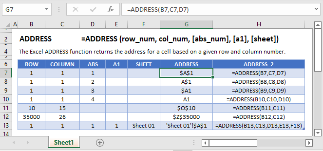
Provide a cell reference by taking a row and column number
What is the Cell ADDRESS Function?
The cell ADDRESS Function[1] is categorized under Excel Lookup and Reference functions. It will provide a cell reference (its “address”) by taking the row number and column letter. The cell reference will be provided as a string of text. The function can return an address in a relative or absolute format and can be used to construct a cell reference inside a formula.
As a financial analyst, cell ADDRESS can be used to convert a column number to a letter, or vice versa. We can use the function to address the first cell or last cell in a range.
Formula
=ADDRESS(row_num, column_num, [abs_num], [a1], [sheet_text])
The formula uses the following arguments:
- Row_num (required argument) – This is a numeric value specifying the row number to be used in the cell reference.
- Column_num (required argument) – A numeric value specifying the column number to be used in the cell reference.
- Abs_num (optional argument) – This is a numeric value specifying the type of reference to return:
| Abs_num | Returns this type of reference |
|---|---|
| 1 or omitted | Absolute |
| 2 | Absolute row; relative column |
| 3 | Absolute column; relative row |
| 4 | Relative |
4. A1(optional argument) – This is a logical value specifying the A1 or R1C1 reference style. In R1C1 reference style, both columns and rows are labeled numerically. It can either be TRUE (reference should be A1) or FALSE (reference should be R1C1).
When omitted, it will take on the default value TRUE (A1 style).
- Sheet_text (optional argument) – Specifies the sheet name. If we omit the argument, it will take the current worksheet.
How to use the ADDRESS Function in Excel?
To understand the uses of the cell ADDRESS function, let us consider a few examples:
Example 1
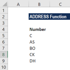
Suppose we wish to convert the following numbers into Excel column references:
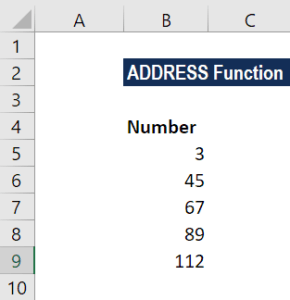
The formula to use will be:
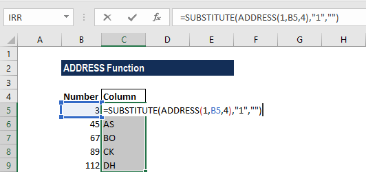
We get the results below:
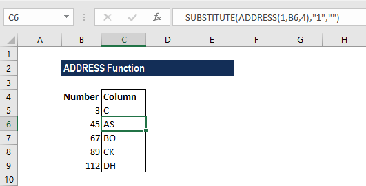
The ADDRESS function will first construct an address containing the column number. It was done by providing 1 for row number, a column number from B6, and 4 for the abs_num argument.
After that, we use the SUBSTITUTE function to take out the number 1 and replace with “”.
Example 2
The ADDRESS function can be used to convert a column letter to a regular number, e.g., 21, 100, 126, etc. We can use a formula based on the INDIRECT and COLUMN functions.
Suppose we are given the following data:
The formula to use will be:
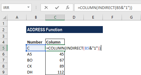
We get the results below:
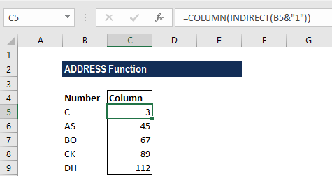
The INDIRECT function transforms the text into a proper Excel reference and hands the result off to the COLUMN function. Then, the COLUMN function evaluates the reference and returns the column number for the reference.
A few notes about the Cell ADDRESS Function
- If we wish to change the reference style that Excel uses, we should go to the File tab, click Options, and then select Formulas. Under Working with formulas, we can select or clear the R1C1 reference style checkbox.
- #VALUE! error – Occurs when any of the arguments are invalid. We would get this argument if:
- The row_num is less than 1 or greater than the number of rows in the spreadsheet;
- The column_num is less than 1 or greater than the number of columns in the spreadsheet; or
- Any of the supplied row_num, column_num or [abs_num] arguments are non-numeric or the supplied [a1] argument is not recognized as a logical value.
Click here to download the sample Excel file
Additional Resources
Thanks for reading CFI’s guide to important Excel functions! By taking the time to learn and master these functions, you’ll significantly speed up your financial analysis. To learn more, check out these additional CFI resources:
- Excel Functions for Finance
- Advanced Excel Formulas Course
- Advanced Excel Formulas You Must Know
- Excel Shortcuts for PC and Mac
- See all Excel resources
Article Sources
- ADDRESS Function
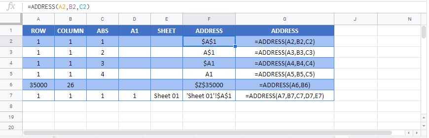
This tutorial demonstrates how to use the ADDRESS Function in Excel and Google Sheets to return a cell address as text.
What is the ADDRESS Function?
The ADDRESS Function Returns a cell address as text.
Usually, in a spreadsheet, we provide a cell reference, and a value from that cell is returned. Instead, the ADDRESS Function builds the name of a cell.
The address can be relative or absolute, in A1 or R1C1 style, and may or may not include the sheet name.
ADDRESS – Basic Example
Let’s say that we want to build a reference to the cell in 4th column and 1st row, aka cell D1. We can use the layout pictured here:
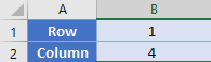
Our formula in A3 is simply
=ADDRESS(B1, B2)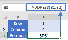
Note: By default the ADDRESS Function returns an absolute cell reference. By updating an optional argument we can change the cell references from absolute to relative. Let’s review this and other inputs to the ADDRESS Function…
ADDRESS Function Syntax and Inputs:
=ADDRESS(row_num,column_num,abs_num,C1,sheet_text)row_num – The row number for the reference. Example: 5 for row 5.
col_num – The column number for the reference. Example: 5 for Column E. You can not enter “E” for column E
abs_num – [optional] A number representing if the reference should have absolute or relative row/column references. 1 for absolute. 2 for absolute row/relative column. 3 for relative row/absolute column. 4 for relative.
a1 – [optional]. A number indicating whether to use standard (A1) cell reference format or R1C1 format. 1/TRUE for Standard (Default). 0/FALSE for R1C1.
sheet_text – [optional] The name of the worksheet to use. Defaults to current sheet.
ADDRESS with INDIRECT
We can combine ADDRESS with the INDIRECT Function. Consider this layout, where we have a list of items in column D.
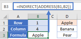
We can generate a reference to D1 like so
=ADDRESS(B1, B2)
=$D$1
By putting the address function inside an INDIRECT function, we’ll be able to use the generated cell reference and use it in a practical way. The INDIRECT will take the reference of “$D$1” and use it to fetch the value from that cell.
=INDIRECT(ADDRESS(B1, B2)
=INDIRECT($D$1)
="Apple"
Note: While the above gives a good example of making the ADDRESS Function useful, it’s not a good formula to use normally. It required two functions, and because of the INDIRECT it will be volatile in nature. A better alternative would have been to use the INDEX Function like this:
=INDEX(1:1048576, B1, B2)
Address of Specific Value
Sometimes when you have a large list of items, you need to know the location of an item in the list. Consider this table of scores from students. We’ve gone ahead and calculated the min, median, and max values of these scores in cells E2:G2.
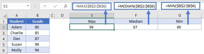
Let’s say we wanted to find these values. We have a two options:
- Filter our table for each of these items.
- Use the MATCH Function with ADDRESS. Remember that MATCH will return the relative position of a value within a range.
Our formula in E3 then is:
=ADDRESS(MATCH(E2, $B:$B, 0), 2)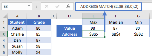
We can copy this same formula across to G3, and only the E2 reference will change since it’s the only relative reference. Looking back at E3, the MATCH function was able to find the value of 98 in the 5th row of column B. Our ADDRESS function then used this to build the full address of “$B$5”.
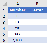
Translate Column Letters from Numbers
So far, all of the examples have returned an absolute reference. Let’s return a relative reference instead.
Below, in column B, we want to calculate the column letter corresponding to the column number in column A.
We will use the ADDRESS Function to return a reference on row 1 in relative format, and then we’ll remove the “1” from the text string so that we just have the letter(s) left. Consider in our table row 3, where our input is 13. Our formula in B3 is
=SUBSTITUTE(ADDRESS(1, A3, 4), "1", "")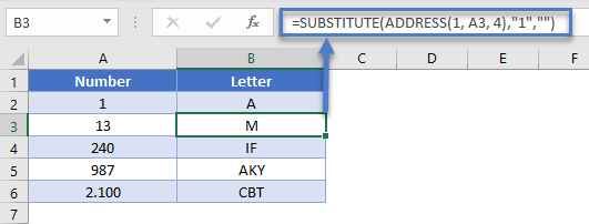
Note that we’ve given the 3rd argument within the ADDRESS function, which controls the relative vs. absolute referencing. The ADDRESS function will output “M1”, and then the SUBSTITUTE function removes the “1” so that we are left with just the “M”.
Find the Address of Named Ranges
In Excel, you can name range or ranges of cells, allowing you to simply refer to the named range instead of the cell reference.
Most named ranges are static, meaning they always refer to the same range. However, you can also create dynamic named ranges that change in size based on some formula(s).
With a dynamic named range, you might need to know the exact address that your named range is pointing to. We can do this with the ADDRESS Function.
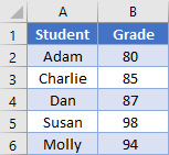
In this example, we’ll look at how to define the address for our named range called “Grades”.
Let’s bring back our table from before:
To get the address of a range, you need to know the top left cell and the bottom left cell. The first part is easy enough to accomplish with the help of the ROW and COLUMN functions. Our formula in E1 can be
=ADDRESS(ROW(Grades), COLUMN(Grades))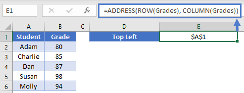
The ROW Function returns the row of the first cell in our range (which will be 1), and the COLUMN will do the same similarly for the column (also 1).
This formula will get the bottom-right cell
=ADDRESS(ROWS(Grades)-ROW(Grades)+1, COLUMNS(Grades)-COLUMN(Grades)+1)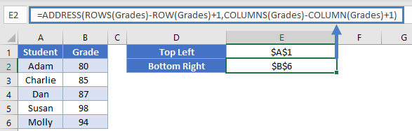
We used the ROWS and COLUMNS functions to calculate the height and width of the range. By subtracting the first row and column numbers, we calculate the last cell in the range
Finally, to put it all together into a single string, we can simply concatenate the values together with a colon in the middle. Formula in E3 can be
=E1 & ":" & E2
Note: While we were able to determine the address of the range, our ADDRESS function determined whether to list the references as relative or absolute. Your dynamic ranges will have relative references that this technique won’t pick up.
2nd Note: This technique only works on a continuous names range. If you had a named range that was defined as something like this formula
=A1:B2, A5:B6then the technique above would result in errors.
ADDRESS function in Google Sheets
The ADDRESS function works exactly the same in Google Sheets as in Excel.