
Excel for Microsoft 365 Excel for Microsoft 365 for Mac Excel for the web Excel 2021 Excel 2021 for Mac Excel 2019 Excel 2019 for Mac Excel 2016 Excel 2016 for Mac Excel 2013 Excel 2010 Excel 2007 Excel for Mac 2011 Excel Starter 2010 More…Less
This article describes the formula syntax and usage of the FIND and FINDB functions in Microsoft Excel.
Description
FIND and FINDB locate one text string within a second text string, and return the number of the starting position of the first text string from the first character of the second text string.
Important:
-
These functions may not be available in all languages.
-
FIND is intended for use with languages that use the single-byte character set (SBCS), whereas FINDB is intended for use with languages that use the double-byte character set (DBCS). The default language setting on your computer affects the return value in the following way:
-
FIND always counts each character, whether single-byte or double-byte, as 1, no matter what the default language setting is.
-
FINDB counts each double-byte character as 2 when you have enabled the editing of a language that supports DBCS and then set it as the default language. Otherwise, FINDB counts each character as 1.
The languages that support DBCS include Japanese, Chinese (Simplified), Chinese (Traditional), and Korean.
Syntax
FIND(find_text, within_text, [start_num])
FINDB(find_text, within_text, [start_num])
The FIND and FINDB function syntax has the following arguments:
-
Find_text Required. The text you want to find.
-
Within_text Required. The text containing the text you want to find.
-
Start_num Optional. Specifies the character at which to start the search. The first character in within_text is character number 1. If you omit start_num, it is assumed to be 1.
Remarks
-
FIND and FINDB are case sensitive and don’t allow wildcard characters. If you don’t want to do a case sensitive search or use wildcard characters, you can use SEARCH and SEARCHB.
-
If find_text is «» (empty text), FIND matches the first character in the search string (that is, the character numbered start_num or 1).
-
Find_text cannot contain any wildcard characters.
-
If find_text does not appear in within_text, FIND and FINDB return the #VALUE! error value.
-
If start_num is not greater than zero, FIND and FINDB return the #VALUE! error value.
-
If start_num is greater than the length of within_text, FIND and FINDB return the #VALUE! error value.
-
Use start_num to skip a specified number of characters. Using FIND as an example, suppose you are working with the text string «AYF0093.YoungMensApparel». To find the number of the first «Y» in the descriptive part of the text string, set start_num equal to 8 so that the serial-number portion of the text is not searched. FIND begins with character 8, finds find_text at the next character, and returns the number 9. FIND always returns the number of characters from the start of within_text, counting the characters you skip if start_num is greater than 1.
Examples
Copy the example data in the following table, and paste it in cell A1 of a new Excel worksheet. For formulas to show results, select them, press F2, and then press Enter. If you need to, you can adjust the column widths to see all the data.
|
Data |
||
|
Miriam McGovern |
||
|
Formula |
Description |
Result |
|
=FIND(«M»,A2) |
Position of the first «M» in cell A2 |
1 |
|
=FIND(«m»,A2) |
Position of the first «M» in cell A2 |
6 |
|
=FIND(«M»,A2,3) |
Position of the first «M» in cell A2, starting with the third character |
8 |
Example 2
|
Data |
||
|
Ceramic Insulators #124-TD45-87 |
||
|
Copper Coils #12-671-6772 |
||
|
Variable Resistors #116010 |
||
|
Formula |
Description (Result) |
Result |
|
=MID(A2,1,FIND(» #»,A2,1)-1) |
Extracts text from position 1 to the position of «#» in cell A2 (Ceramic Insulators) |
Ceramic Insulators |
|
=MID(A3,1,FIND(» #»,A3,1)-1) |
Extracts text from position 1 to the position of «#» in cell A3 (Copper Coils) |
Copper Coils |
|
=MID(A4,1,FIND(» #»,A4,1)-1) |
Extracts text from position 1 to the position of «#» in cell A4 (Variable Resistors) |
Variable Resistors |
Need more help?
Want more options?
Explore subscription benefits, browse training courses, learn how to secure your device, and more.
Communities help you ask and answer questions, give feedback, and hear from experts with rich knowledge.
Excel FIND Function (Example + Video)
When to use Excel FIND Function
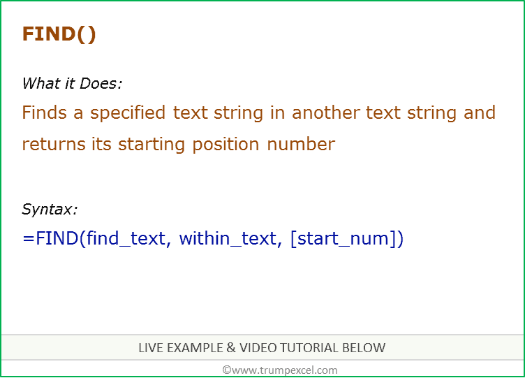
Excel FIND function can be used when you want to locate a text string within another text string and find its position.
What it Returns
It returns a number that represents the starting position of the string you are finding in another string.
Syntax
=FIND(find_text, within_text, [start_num])
Input Arguments
- find_text – the text or string that you need to find.
- within_text – the text within which you want to find the find_text argument.
- [start_num] – a number that represents the position from which you want the search to begin. If you omit it, it starts from the beginning.
Additional Notes
- If the start number is not specified, then it starts looking from the beginning of the string.
- Excel FIND function is case-sensitive. If you want to do a case-insensitive search, use Excel SEARCH function.
- Excel FIND function cannot handle wildcard characters. If you want to use wildcard characters, use the Excel SEARCH function.
- It returns a #VALUE! error if the searched string is not found in the text.
Excel FIND Function – Examples
Here are four examples of using Excel FIND function:
Searching for a Word in a Text String (from the beginning)
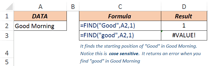
In the above example, when you look for the word Good in the text Good Morning, it returns 1, which is the position of the starting point of the searched word.
Note that Excel FIND function is case-sensitive. When you use good instead of Good, it returns a #VALUE! error.
If you are looking for a case-insensitive search, use Excel SEARCH function.
Finding a Word in a Text String (with a specified beginning)
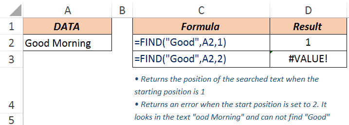
The third argument in the FIND function is the position within the text from where you want to start the search. In the example above, the function returns 1 when you search for the text Good in Good Morning and the starting position is 1.
However, it returns an error when you make it start at 2. Hence, it looks for the text Good in ood Morning. Since it can not find it, it returns an error.
Note: If you skip the last argument and don’t provide the starting position, by default it takes it as 1.
When there are Multiple Occurrence of the Searched Text
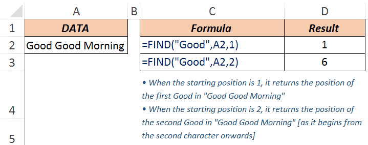
Excel FIND function starts looking in the specified text from the specified position. In the above example, when you look for the text Good in Good Good Morning with the starting position as 1, it returns 1, as it finds it at the beginning.
When you start the search from the second character onwards, it returns 6, as it finds the matching text at the sixth position.
Extracting Everything to the Left a Specified Character/String
Suppose you have the email ids do some superheroes as shown below and you want to extract only the username part (which would be the characters before the @).
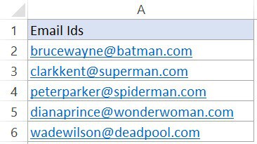
Below is the formula that will find the position of ‘@’ in each email id and extract all the characters to the left of it:
=LEFT(A2,FIND(“@”,A2,1)-1)

The FIND function in this formula gives the position of the ‘@’ character. The LEFT function that uses this position to extract the username.
For example, in the case of brucewayne@batman.com, the FIND function returns 11. LEFT function then uses FIND(“@”,A2,1)-1 as the second argument to get the username.
Note that 1 is subtracted from the value returned by the FIND function as we want to exclude the @ from the result of the LEFT function.
Excel FIND Function – VIDEO
Related Excel Functions:
- Excel LOWER Function.
- Excel UPPER Function.
- Excel PROPER Function.
- Excel REPLACE Function.
- Excel SEARCH Function.
- Excel SUBSTITUTE Function.
You May Also Like the Following Tutorials:
- How to Quickly Find and Remove Hyperlinks in Excel.
- How to Find Merged Cells in Excel.
- How to Find and Remove Duplicates in Excel.
- Using Find and Replace in Excel.
Find in Excel (Table of Contents)
- Using Find and Select Feature in Excel
- FIND Function in Excel
- SEARCH Function in Excel
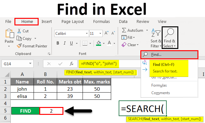
Introduction to Find in Excel
There are two ways to find it in Excel. First, we can use Find by pressing Ctrl + F shortcut keys. Therein Find and Replace box, search the word or field which we want to find in the Find What section. In another way, we can use the FIND function. For this, select the Find function from the insert function and, as per syntax, select the substring from where we need to find it, and choose the word or letter or number which we want to find in the String position. This will return the position of the chosen string from the selected Substring.
Methods to Find in Excel
Below are the different methods to find in excel.
You can download this Find in Excel Template here – Find in Excel Template
Method #1 – Using Find and Select Feature in Excel
Let’s see How to Find a Number or a Character in Excel using the Find and Select feature in Excel.
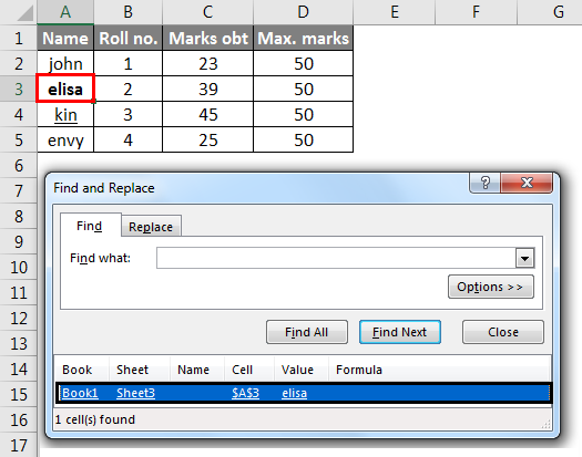
Step 1 – Under the Home tab, in the Editing group, click Find & Select.
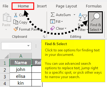
Step 2 – To find text or numbers, click Find.
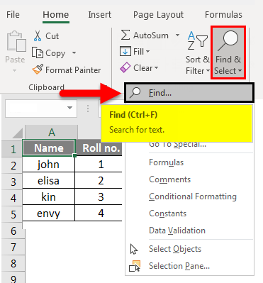
- In the Find what box, type the text or character you want to search for, or click the arrow in the Find what box and then click a recent search in the list.
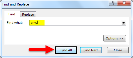
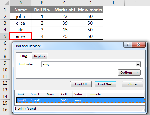
Here, we have a record of marks of four students. Suppose we want to find the text ‘envy’ in this table. For this, we click Find and Select under the Home tab then the Find and Replace dialog box appears. In the Find what box, we enter ‘envy’ then click on Find All. We get the text ‘envy’ is in cell number A5.
- You can use wildcard characters, such as an asterisk (*) or a question mark (?), in your search criteria:
Use the asterisk to find any string of characters.
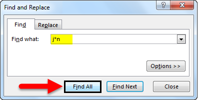
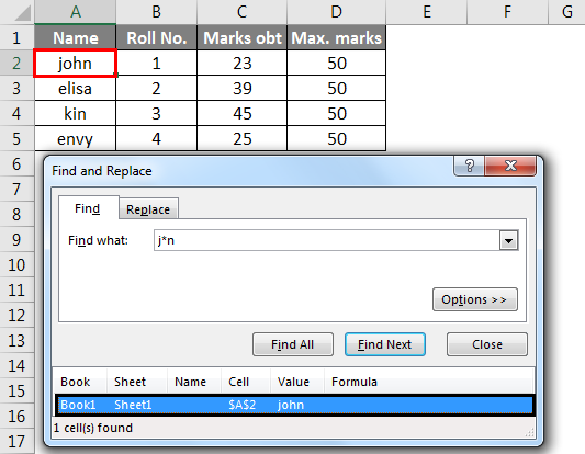
Suppose we want to find text in the table which starts with the letter ‘j’ and ends with the letter ‘n’. In the Find and Replace dialog box, we enter ‘j*n’ in the Find what box, then click on Find All.
We will get the result as text ‘j*n’(john) is in the cell no. ‘A2’ because we have only one text which starts with ‘j’ and ends with ‘n’ with any number of characters between them.
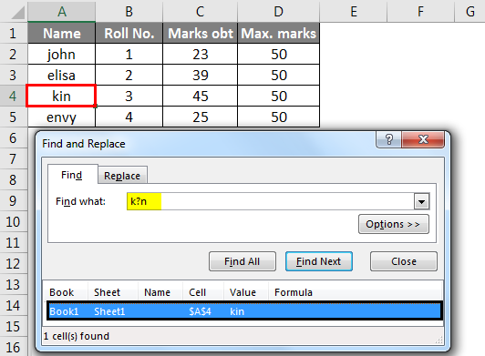
Use the question mark to find any single character.
Suppose we want to find text in the table that starts with the letter ‘k’ and ends with the letter ‘n’ with a single character. So, in the Find and Replace dialog box, we enter ‘k?n’ to find what box. Then click on Find All.
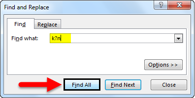
Here, we get the text ‘k?n’(kin) is in cell no. ‘A4’ because we have only one text which starts with ‘k’ and ends with ‘n’ with a single character between them.
- Click Options to further define your search if needed.
- We can find text or number by changing settings in the Within, Search and Look in the box according to our needs.
- To show the working of the above-mentioned options, we took the data as follows.
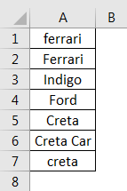
- To search case-sensitive data, select the Match case check box. It gives you output in the case you give input in the Find What box. For example, we have a table of some cars’ names. If you type ‘ferrari’ in the Find What box, then it will find only ‘ferrari’, not ‘Ferrari’.
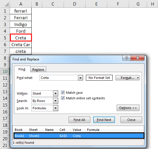
- To search for cells that contain just the characters you typed in the Find what box, select the Match entire cell contents checkbox. For example, we have a table of some cars’ names. Type ‘Creta’ in the Find What box.
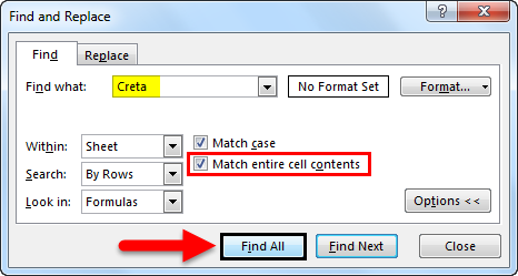
- It will then find cells containing exactly ‘Creta’, and cells containing ‘Cretaa’ or ‘Creta car’ will not be found.
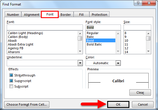
- If you want to search for text or numbers with specific formatting, click Format, and then make your selections in the Find Format dialog box according to your need.
- Let us click the Font option and select the Bold, and click OK.
- Then, we click on Find All.
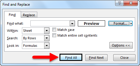
We get the value as ‘elisa’, which is in the ‘A3’ cell.
Method #2 – Using FIND Function in Excel
The FIND function in Excel gives the location of a substring within a string.
Syntax For FIND in Excel:
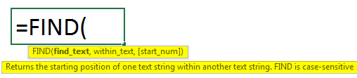
The first two parameters are required, and the last parameter is non-compulsory.
- Find_Value: The substring which you want to find.
- Within_String: The string in which you want to find the specific substring.
- Start_Position: It is a non-compulsory parameter and describes from which position we want to search substring. If you do not describe it, then start the search from the 1st position.
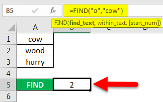
For example =FIND(“o”, “Cow”) gives 2 because “o” is the 2nd letter in the word “cow“.
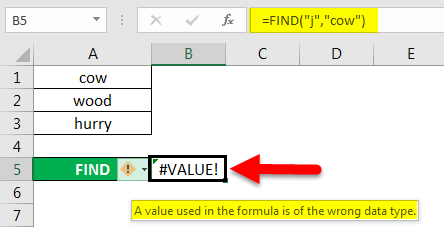
FIND(“j”, “Cow”) gives an error because there is no “j” in “Cow”.
- If the Find_Value parameter contains multiple characters, the FIND function gives the location of the first character.
E.g., the formula FIND(“ur”, “hurry”) gives 2 because “u” in the 2nd letter in the word “hurry”.

- If Within_String contains multiple occurrences of Find_Value, the first occurrence is returned. For example, FIND (“o”, “wood”)
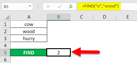
gives 2, which is the location of the first “o” character in the string “wood”.
The Excel FIND function gives the #VALUE! error if:
- If Find_Value does not exist in Within_String.
- If Start_Position contains multiple characters as compared to Within_String.
- If Start_Position either has a zero or negative number.
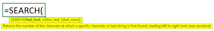
Method #3 – Using SEARCH Function in Excel
The SEARCH function in Excel is simultaneous to FIND because it also gives the location of a substring in a string.
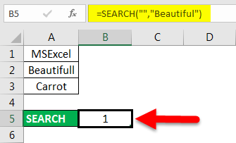
- If Find_Value is the blank string “, the Excel FIND formula gives the string’s first character.
Example =SEARCH (“ful“, “Beautiful) gives 7 because the substring “ful” begins at the 7th position of the substring “beautiful”.
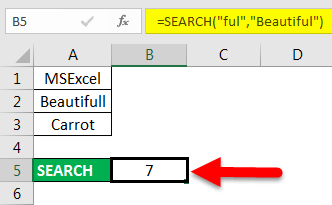
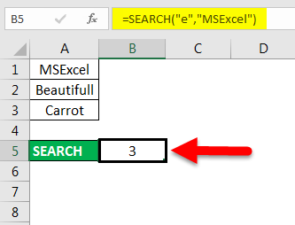
=SEARCH (“e”, “MSExcel”) gives 3 because “e” is the 3rd character in the word “MSExcel” and ignoring the case.
- Excel’s SEARCH function gives the #VALUE! error if:
- If the value of the Find_Value parameter is not found.
- If the Start_Position parameter is superior to the length of Within_String.
- If the Start_Position either equal to or less than 0.
Things to Remember About Find in Excel
- Asterisk defines a string of characters, and the question mark defines a single character. You can also find asterisks, question marks, and tilde characters (~) in worksheet data by preceding them with a tilde character inside the Find what option.
For example, to find data that contain “*”, you would type ~* as your search criteria.
- If you want to find cells that match a specific format, you can delete any criteria in the Find what box and select a specific cell format as an example. Click the arrow next to Format, click Choose Format From Cell, and click the cell with the formatting you want to search for.
- MSExcel saves the formatting options you define; you should clear the formatting options from the last search by clicking on an arrow next to Format and then Clear Find Format.
- The FIND function is case sensitive and does not allow while using wildcard characters.
- The SEARCH function is case-insensitive and allows while using wildcard characters.
Recommended Articles
This is a guide to Find in Excel. Here we discuss how to use the Find feature, Formula for FIND, and SEARCH in Excel, along with practical examples and a downloadable excel template. You can also go through our other suggested articles –
- FIND Function in Excel
- Excel SEARCH Function
- Find and Replace in Excel
- Search For Text in Excel
The FIND function is a built-in Worksheet Function (WS) in Microsoft Excel, which you can use to locate a sub-string or a specific character’s position within a text string. It is categorized as a TEXT function in Excel.
If the FIND function fails to find the text, it will return a #VALUE error. Note that the Excel FIND function will perform a case-sensitive search.
Excel FIND function is commonly used by financial analysts for locating specific data or text occurrences in a cell.

Syntax of Excel FIND function
=FIND(find_text, within_text, [start_num])
Arguments:
'find_text' – The text/sub-string you want to locate.'within_text' – This argument is the string within which you wish to perform the search. You can supply a cell reference or type in the string into the formula.'start_num' – This is an optional argument wherein you specify the character from which your search must begin. If you omit this argument, the function will assume this parameter as 1, i.e., the search will begin from the 1st character of the 'within_text' string.
Things to Remember
- The FIND function in Excel is case-sensitive and does not allow the usage of wildcard characters. For locating case-insensitive matches, take a look at the SEARCH function.
- The FIND function will search the
'find_text'argument in'within_text'and return the first character’s position. - You may search for either a substring or a character with the
'find_text'argument. You may use cell references or text characters for both'find_text'and'within_text'The FIND function will return ‘1’ when the'find_text'argument is an empty string «». - The FIND function returns #VALUE! error when:
- The FIND function cannot locate
'find_text'in'within_text'or - The
'start_num'argument is negative, 0, or greater than the length of'within_text'
- The FIND function cannot locate
Examples of FIND function in Excel
Example 1 – Finding a word’s position in a text string

In this example, when you search for «Dallas» and reference the cell A2, which has the text string «Dallas, USA» the function will return ‘1’. Here, 1 represents the position of the searched word’s starting point.
On account of the FIND function’s case-sensitivity, entering «dallas» as an argument will return #VALUE! error.
Example 2 – Search for a word in a text string

The 'start_num' argument lets you decide the starting position for performing the search in the text string. You will see that in the above example, the FIND function returns ‘1’ when we put 1 as the 'start_num'. Essentially, it searches for the text «Dallas» in «Dallas, USA».
When we change 'start_num' to ‘2’, it returns an error because it then searches for «Dallas» in «allas, USA».
Note that skipping the 'start_num' argument will result in the FIND function assuming ‘1’ as the starting position.
Example 3 – When the searched text occurs multiple times in a text string

Since the FIND function refers to the 'start_num' argument to see if you would like to define a starting position, it returns ‘1’ when you input 'start_num' as 1. This is because it finds «Dallas» at position ‘1’ in «Dallas, Dallas, USA».
When you input 'start_num' as 2, though, you will see that it returns ‘9’. What is happening here is that the FIND function tries to look for the word «Dallas» in «allas, Dallas, USA» since you are asking the function to start searching from the second position. Here, 9 is the starting position of the 2nd «Dallas» in «Dallas, Dallas, USA».
Example 4 – Look for a specific character’s Nth occurrence in a string.

Let’s now assume that you would like to know the position of the second «,» in the list that has the format «City, Country, Continent».
For this, we will need to nest two FIND functions one within another. The second FIND function will go in the first FIND function as a third argument ('start_num'), like so:
=FIND(",",A2,FIND(",",A2)+1)
With the third argument, you are instructing the first FIND function to start searching for «,» exactly after the first occurrence of a «,» in the string.
Pro tip: You can use the CHAR and SUBSTITUTE functions to do this more simply, with the following formula:
=FIND(CHAR(1), SUBSTITUTE(A5,",",CHAR(1),2)
Example 5 – Retrieving the first part of a text string separated by «,» (comma)

Let’s assume you want the list of just the name of cities, without the name of the country, i.e., the characters right before «,»).
To accomplish this, we will use the LEFT function and the FIND function together. The FIND function will give us the position of «,» and the LEFT function will allow us to retrieve the name of the cities.
In our example, the FIND function will return 10 when executed on «Amsterdam, Netherlands». From this, we will subtract 1 since we don’t want to include the «,» in our output.
Next, we embed a FIND function into the LEFT function and use FIND(",", A2,1)-1 as the second argument, like so:
=LEFT(A2,FIND(",",A2,1)-1)
Example 6 – Retrieving the second part of a text string separated by «,» (comma)

Let’s take example 5, and try to retrieve the second part of the string.
To accomplish this, we will use the MID function and the FIND function together. The FIND function will give us the position of «,» and the MID function will allow us to fetch the specific string portion that we need.
In our example, the FIND function will return 10 when executed on «Amsterdam, Netherlands». From this, we will add 1 since we don’t want to include the «,» in our output.
Next, we use a MID function and pass the FIND function to it FIND(",", A2,1)+1 as the second argument, like so:
=MID(A2,FIND(",",A2,1)+1,100)
FIND function vs. SEARCH function in Excel
Both Find and Search functions have a similar syntax and application. However, there are 2 differences between these functions. Let’s dive into what these differences are:
1. Acceptance of wildcard characters
Unlike with the FIND function, you may use wildcard characters in the SEARCH function’s 'find_text' argument.
To match one character – we will use a question mark ‘?’, and to match a series of characters – we will use an asterisk mark ‘*’.
Let’s work this out with an example:

We will use the syntax:
=SEARCH(",*EUROPE",A2)
Notice how the Excel SEARCH function returns the first character’s position if you input both «,» and the «continent name» regardless of how many characters exist between the text string referred to in the 'within_text'argument.
Pro tip: For finding a ‘?’ or ‘*’, just add a tilde (~) in front of the question mark or the asterisk.
2. FIND is case-sensitive, while SEARCH is case-insensitive
As I mentioned previously, case-sensitivity is another differentiating factor between the two functions.

In our example, when using the FIND function to search for ‘A’ it returns the position of the capital A in ‘USA’. However, searching for ‘A’ with the SEARCH function returns the position of the ‘a’ in ‘Dallas’ because it is case-insensitive.
Handling #VALUE! errors in the FIND function
To deal with #VALUE! errors, we can use the IFERROR function.
Let’s revisit our first example where we first encountered a #VALUE! error with FIND function on account of the FIND function’s case-sensitivity.

Here is the syntax we will use to fix this:
=IFERROR(FIND("dallas",A3,1), "Not Found!")
Using this syntax, we will «trap» the error and replace it with a standard string in the second argument of the IFERROR function, which in our case is «Not Found!». So, until the FIND function is able to return a matched string, the function will keep returning «Not Found».
Функция НАЙТИ (FIND) в Excel используется для поиска текстового значения внутри строчки с текстом и указать порядковый номер буквы с которого начинается искомое слово в найденной строке.
Содержание
- Что возвращает функция
- Синтаксис
- Аргументы функции
- Дополнительная информация
- Примеры использования функции НАЙТИ в Excel
- Пример 1. Ищем слово в текстовой строке (с начала строки)
- Пример 2. Ищем слово в текстовой строке (с заданным порядковым номером старта поиска)
- Пример 3. Поиск текстового значения внутри текстовой строки с дублированным искомым значением
Что возвращает функция
Возвращает числовое значение, обозначающее стартовую позицию текстовой строчки внутри другой текстовой строчки.
Синтаксис
=FIND(find_text, within_text, [start_num]) — английская версия
=НАЙТИ(искомый_текст;просматриваемый_текст;[нач_позиция]) — русская версия
Аргументы функции
- find_text (искомый_текст) — текст или строка которую вы хотите найти в рамках другой строки;
- within_text (просматриваемый_текст) — текст, внутри которого вы хотите найти аргумент find_text (искомый_текст);
- [start_num] ([нач_позиция]) — число, отображающее позицию, с которой вы хотите начать поиск. Если аргумент не указать, то поиск начнется сначала.
Дополнительная информация
- Если стартовое число не указано, то функция начинает поиск искомого текста с начала строки;
- Функция НАЙТИ чувствительна к регистру. Если вы хотите сделать поиск без учета регистра, используйте функцию SEARCH в Excel;
- Функция не учитывает подстановочные знаки при поиске. Если вы хотите использовать подстановочные знаки для поиска, используйте функцию SEARCH в Excel;
- Функция каждый раз возвращает ошибку, когда не находит искомый текст в заданной строке.
Примеры использования функции НАЙТИ в Excel
Пример 1. Ищем слово в текстовой строке (с начала строки)

На примере выше мы ищем слово «Доброе» в словосочетании «Доброе Утро». По результатам поиска, функция выдает число «1», которое обозначает, что слово «Доброе» начинается с первой по очереди буквы в, заданной в качестве области поиска, текстовой строке.
Больше лайфхаков в нашем Telegram Подписаться
Обратите внимание, что так как функция НАЙТИ в Excel чувствительна к регистру, вы не сможете найти слово «доброе» в словосочетании «Доброе утро», так как оно написано с маленькой буквы. Для того, чтобы осуществить поиска без учета регистра следует пользоваться функцией SEARCH.
Пример 2. Ищем слово в текстовой строке (с заданным порядковым номером старта поиска)
Третий аргумент функции НАЙТИ указывает позицию, с которой функция начинает поиск искомого значения. На примере выше функция возвращает число «1» когда мы начинаем поиск слова «Доброе» в словосочетании «Доброе утро» с начала текстовой строки. Но если мы зададим аргумент функции start_num (нач_позиция) со значением «2», то функция выдаст ошибку, так как начиная поиск со второй буквы текстовой строки, она не может ничего найти.
Если вы не укажете номер позиции, с которой функции следует начинать поиск искомого аргумента, то Excel по умолчанию начнет поиск с самого начала текстовой строки.
Пример 3. Поиск текстового значения внутри текстовой строки с дублированным искомым значением
На примере выше мы ищем слово «Доброе» в словосочетании «Доброе Доброе утро». Когда мы начинаем поиск слова «Доброе» с начала текстовой строки, то функция выдает число «1», так как первое слово «Доброе» начинается с первой буквы в словосочетании «Доброе Доброе утро».
Но, если мы укажем в качестве аргумента start_num (нач_позиция) число «2» и попросим функцию начать поиск со второй буквы в заданной текстовой строке, то функция выдаст число «6», так как Excel находит искомое слово «Доброе» начиная со второй буквы словосочетания «Доброе Доброе утро» только на 6 позиции.