
How to Sum by Color in Excel? (2 Useful Methods)
The top two methods to Sum by Colors in Excel are as follows –
- Usage of SUBTOTAL formula in excelThe SUBTOTAL excel function performs different arithmetic operations like average, product, sum, standard deviation, variance etc., on a defined range.read more and filter by color function.
- Applying GET.CELL formula by defining the name in the formula tab and applying the SUMIF formula in excelThe SUMIF Excel function calculates the sum of a range of cells based on given criteria. The criteria can include dates, numbers, and text. For example, the formula “=SUMIF(B1:B5, “<=12”)” adds the values in the cell range B1:B5, which are less than or equal to 12.
read more to summarize the values by color codes.
Let us discuss each of them in detail –
Table of contents
- How to Sum by Color in Excel? (2 Useful Methods)
- #1 – Sum by Color using Subtotal Function
- #2 – Sum by Color using Get.Cell Function
- Things to Remember
- Recommended Articles
You can download this Sum by Color Excel Template here – Sum by Color Excel Template
#1 – Sum by Color using SUBTOTAL Function
To understand the approach for calculating the sum of values by background colors, let us consider the below data table, which provides details of amounts in US$ by region and month.

Lets start.
- Suppose we would like to highlight those cells which are negative in values for indication purpose, this can be achieved by either applying conditional formatting or manually highlighting the cells, as shown below.

- To achieve the sum of cells that are colored in excel, enter the formula for SUBTOTAL below the data table. The syntax for the SUBTOTAL formula is shown below.

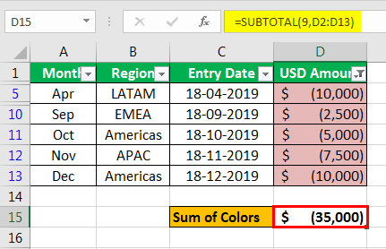
The formula that is entered to calculate the summation is=SUBTOTAL(9,D2:D13)
Here, the number 9 in the function_num argument refers to sum functionality, and the reference argument is given as the range of cells to be computed. Below is the screenshot for the same.

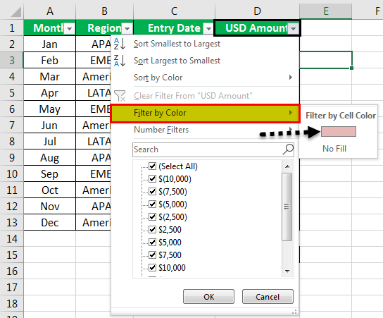
- As the above screenshot shows, a “USD Amount” summation has been calculated to compute the amounts highlighted in a light red background. Next, apply the filter to the data table by going to the “Data” tab and selecting a filter.

- Select filter by color and choose the light red cell color under “Filter by Color.” Below is the screenshot to better describe the filter.

- Once the excel filter has been applied, it will filter the data table for only light red background cells. The subtotal formula used at the bottom of the data table would display the summation of the colored cells, which are filtered as shown below.

As shown in the above screenshot, the computation of the colored cell is achieved in cell E17, subtotal formula.


#2 – Sum by Color using Get.Cell Function
The second approach is explained to arrive at the sum of the color cells in excel, as discussed in the below example. Consider the data tableA data table in excel is a type of what-if analysis tool that allows you to compare variables and see how they impact the result and overall data. It can be found under the data tab in the what-if analysis section.read more to understand the methodology better.

- Step 1: Now, let us highlight the list of cells in the “USD Amount” column, which we are willing to arrive at the desired sum of colored cells, as shown below..

- Step 2: As we can see in the above screenshot, unlike in the first example here, we have multiple colors. Thereby we will be using the formula =GET.CELL by defining it within the name boxIn Excel, the name box is located on the left side of the window and is used to give a name to a table or a cell. The name is usually the row character followed by the column number, such as cell A1.read more and not directly using it in excel.
- Step 3: Now, once the dialog box for the “Define Name” pops up, enter the name and the formula forgetting. CELL in “Refer to,” as shown in the below screenshot.
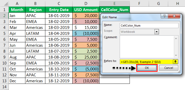
As seen in the above screenshot, the name entered for the function is “CellColor_Num,” and the formula =GET.CELL(38,’Example 2!$D2) is to be entered in ‘Refers to.’ Within the formula, the numeric 38 refers to the cell code information, and the second argument is the cell number D2 refers to the reference cell. Now, click “OK.”
- Step 4: Now, enter the function name “CellColor” in the cell beside the color-coded cell, which was defined in the dialog box, as explained in step 3.

As seen in the above screenshot, the function “CellColor” is entered, which returns the color code for the background cell color.
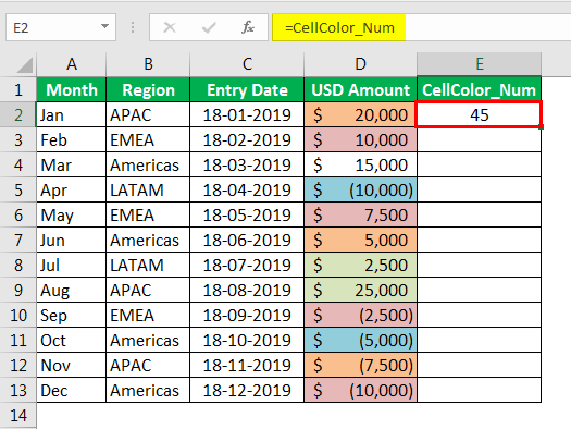
Similarly, the formula is dragged for the entire column.

- Step 5: Now, to arrive at the sum of the values by colors in excel, we will be entering the SUMIF formula. The syntax for the SUMIF formula is as follows:-

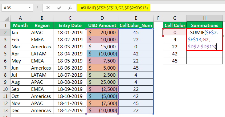
As can be seen from the above screenshot, the following arguments are entered into the SUMIF formula:-
- The range argument is entered for cell range E2: E13.
- The criteria are entered as G2, whose summarized values are needed to be retrieved.
- The range of cells is entered to be D2: D13.
The SUMIF formula is dragged down for all the color code numbers for which values are to be added together.

Things to Remember
- While using the approach by SUBTOTAL formula, this functionality allows the users to filter for only one color at a time. Moreover, we can utilize this functionality to add only one column of values by filtering colors if there is more than one column with different colors by rows in the various columns. The SUBTOTAL may only show the correct result for one filter by color to a specific column.
- The GET.CELL formula, combined with the SUMIF approach, eliminates this limitation, as we could use this functionality to summarize by colors for multiple color codes in the cell background.
Recommended Articles
This article is a guide to Sum by Color in Excel. Here, we discuss how to find sum by colors in Excel using 1) SUBTOTAL Function and 2) Get. Cell, along with practical examples and a downloadable Excel template. You may learn more about Excel from the following articles: –
- Excel SUM ShortcutsThe Excel SUM Shortcut is a function that is used to add up multiple values by simultaneously pressing the “Alt” and “=” buttons in the desired cell. However, the data must be present in a continuous range for this function to function.read more
- Excel SUMIF Between Two DatesWhen we wish to work with data that has serial numbers with different dates and the condition to sum the values is based between two dates, we use Sumif between two dates. read more
- Excel VBA Color IndexVBA Colour Index is used to change the colours of cells or cell ranges. This function has unique identification for different types of colours.read more
- Sort by Color in ExcelWhen a column or a data range in excel is formatted with colors either by using the conditional formatting or manually, when we use filter on the data excel provides us with an option to sort the data by color, there is also an option for advanced sort where user can enter different levels of color for sorting.read more
Excel has some really amazing functions, but it doesn’t have a function that can sum cell values based on the cell color.
For example, I have the dataset as shown below, and I want to get the sum of all orange and yellow color cells.

Unfortunately, there is no in-built function to do this.
But never say never!
In this tutorial, I will show you three simple techniques you can use to sum by color in Excel.
Let’s dive in!
SUM Cells by Color Using Filter and SUBTOTAL
Let’s start with the easiest one.
Below I have a dataset where I have the employee names and their sales numbers.
And in this dataset, I want to get the sum of all the cells colored in yellow and orange.
While there is no in-built function in Excel to sum values based on cell color, there is a simple workaround that relies on the fact that you can filter cells based on the cell color.
For this method, enter the below formula in cell B17 (or any cell in the same column below the colored cells dataset).
=SUBTOTAL(9,B2:B15)

In the above SUBTOTAL formula, I have used 9 as the first argument, which tells the function that I want to get the sum of the range that is given as the second argument.
But why not just use the SUM formula instead?
This is because when I have the SUBTOTAL formula and I filter the cells to only show those cells that have a specific color in it, the SUBTOTAL formula will show me the sum of visible cells only (something that the SUM formula can not do).
So once you have the SUBTOTAL formula, follow the below steps to get the SUM based on cell color:
- Select any cell in the dataset
- Click the Data tab

- In the Sort and Filter group, click on the Filter icon. This will apply filter to the dataset and you will be able to see the filter icon in the headers
- In the Sales header cell, click on the Filter icon
- Go to the Filter by Color” option
- Select the color based on which you want to filter the dataset.

As soon as you do this, you will notice that the subtotal result changes and it will now only give you the sum of those cells that are visible (which would only be those cells that have the color by which you filtered the dataset).

Similarly, if you filter by some other color in the data set (say orange instead of yellow), the SUBTOTAL function would accordingly adjust and give you the sum of all cells with orange color
Pro Tip: Keyboard shortcut to apply a filter to a dataset is Control + Shift + L (hold the Control and the Shift key, and then press the L key). If using Mac, use Command + Shift + L
SUM Cells by Color Using VBA
I mentioned that there is no inbuilt formula in Excel to sum based on cell color value. However, you can create your own formula to do this using VBA.
With VBA, you can create a custom function that you can keep in the back end, and then use it like any other regular function in the worksheet.
Below is the VBA code that will create that custom function that allows you to sum by color in Excel.
'Code created by Sumit Bansal from https://trumpexcel.com/
'This VBA code created a function that can be used to sum cells based on color
Function SumByColor(SumRange As Range, SumColor As Range)
Dim SumColorValue As Integer
Dim TotalSum As Long
SumColorValue = SumColor.Interior.ColorIndex
Set rCell = SumRange
For Each rCell In SumRange
If rCell.Interior.ColorIndex = SumColorValue Then
TotalSum = TotalSum + rCell.Value
End If
Next rCell
SumByColor = TotalSum
End Function
To use this VBA custom function, you will first have to copy this code and paste it in the back end in the VB editor.
Once done, you’ll be able to use this function in the worksheet.
Below are the steps to add this code to the VB editor.
- Click the Developer tab in the ribbon (if you don’t have the Developer tab visible, click here to learn how to get it)
- Click on the Visual Basic icon. This will open the Visual Basic editor of Excel.

- Click the Insert option in the menu
- Click on Module. This will insert a new module and you will be able to see it in the project explorer (a pane on the left that shows all the objects). If you don’t see the Project Explorer pane, click on View and then click on Project Explorer

- Copy the above VBA code and paste it in the newly inserted Module code window

- Close the VB Editor
Now that you have the code in the back end in excel, you will be able to use the function that we created (SumByColor) in the worksheet.
For this function to work, I will need a cell in the worksheet that contains the same color for which I want to get the sum.
In our example, I have done that to cells D2 and D3, where D2 has the yellow color and D3 has the orange color.
Now I can use the below formula in these cells:
=SumByColor($B$2:$B$15,D2)

The above formula takes two arguments:
- The range of cells that have the color that I want to add
- Reference to any cell that contains the color (so that the formula can pick the color index and use that as a condition to add the values)
Note that the formula is dynamic and would automatically update in case you make any changes to the data set (such as changing any value or applying/removing color from some cells). And in case you notice that the formula is not updating, hit the F9 key and it would update.
Since we have used a VBA code in the workbook, it needs to be saved as a macro-enabled workbook (with .XLSM extension).
Pro Tip: If adding cells based on their background color is something you need to do quite often, I recommend you copy and paste this VBA code for the custom formula in the Personal Macro Workbook. This way, that would be available on all your workbooks on your system.
Also read: Filter By Color in Excel
SUM Cells by Color Using GET.CELL
The final method I want to show you include a hidden Excel formula (that not many people know about).
This method uses the GET.CELL function, which can get us the color index value of colored cells.
And once we have the color index value of each cell, we can then use a simple sum if formula to only get the sum of cells with a specific color in it.
It’s not as elegant as the VBA custom function I covered earlier, but if you don’t want to use VBA, then this could be the way to go for you.
GET.CELL is an old Macro 4 function that has been kept in Excel for compatibility reasons, but you won’t find many details about it (as it’s rarely used).
Below I have a dataset where I have colored cells that I want to sum.
For this technique to work, we first need to create a named range that will use the GET.CELL function to give the color value of a colored cell.
Here are the steps to do this:
- Click the Formulas tab in the Ribbon
- In the Defined Names group, click on the ‘Name Manager’

- In the Name Manager dialog box, click on New

- In the ‘New Name dialog box, enter the Name – SumColor

- In the Refers to field, enter the following formula: =GET.CELL(38,$B2)

- Click OK
- Close the Name Manager dialog box
The above steps have created a named range that we can now use in the workbook.
Note: GET.CELL function takes two arguments, the first one is a number that tells the function what information we need, and the second is the cell reference of that cell itself. In this case, I have 38 as the first argument, which would give us the color index value of the referred cell.
Now the second step is to get the color index values of all the colors in column B.
Below are the steps to do this:
- In cell C1, enter the header – Color Index (or anything that you to call it)

- In cell C2, enter the following formula: =SumColor

- Apply the same formula for all the cell in column C (you can use the fill handle or simply copy paste cell C2)

The above steps would give you a value that would represent the color index of the cell in column B (the cell on the left).
SumColor is the named range we created and it uses the GET.CELL function to get the color index value of the cell on the left. You can use this formula in any column, but it should always start from the second cell in that column. For example, instead of column C, you can have this in column H or J, but from the second cells in these columns.
Now that we have a unique number for each color, we can use this to get the SUM of cells based on their color.
Below are the steps to do this:
- In cell E2 and E3, give the cells the color for which you want to get the sum. In my case, I have yellow color in cell E2 and orange in cell E3

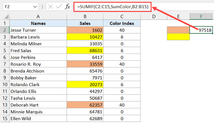
- In cell F2, enter the following formula: =SUMIF(C2:C15,SumColor,B2:B15)
- Copy the cell and paste in cell F3 (this could copy the formula as well and adjust the references).

The above steps would give you the sum of all the cells that have the color in the adjacent selling column F.
We have used a SUMIF formula, where it adds all the values in column B, if the color index of the cell on the left (in column F) is the same as that in column C.
While this is definitely a slightly longer way to sum cells by color (as compared with SUBTOTAL or VBA), this gets the work done, and you only need to do this setup once.
Note that while the formula is dynamic, in case you make any changes (such as changing the color cells in column B or removing the color from it), the change might not be reflected instantly in the SUMIF formula. A simple workaround for it would be to go to the cell that has the formula, click the F2 key to get into the airport, and then hit the enter key. This would force the formula to recalculate and you will get the updated result.
So these are three methods you can use to sum by color in Excel. While SUBTOTAL is quite easy and straightforward, I personally like the VBA method better.
I hope you found this tutorial useful!
Other Excel tutorials you may also like:
- Count Characters in a Cell (or Range of Cells) Using Formulas in Excel
- How to Count Colored Cells in Excel
- How to Sort By Color in Excel (in less than 10 seconds)
- How to Apply Formula to Entire Column in Excel
- How to Sum Only Positive or Negative Numbers in Excel (Easy Formula)
- How to SUM values between two dates (using SUMIFS formula)
- How to Combine Duplicate Rows and Sum the Values in Excel
- How to Sum Across Multiple Sheets in Excel? (3D SUM Formula)
How to SUM by color in Excel: Step-by-Step Guide (2023)
Most of you know how to get the Excel SUM. It’s one of the most basic Excel functions.
What most people don’t know is that you can get the Excel SUM by color, too 🤩
There is no built-in function for this but it doesn’t mean Excel can’t 😉
Today, you’re in for a colorful, in-depth lesson on how to SUM by color in Excel.
Let’s go!
SUM cells by color with filter and total
The contribution made by association members to a project is displayed in the Excel table below 💰

The amount that has yet to be collected is indicated in the highlighted cells.
Let’s say you want to know the total of the cells that have been highlighted.
You can find the total value of all the colored cells by following the steps below 👍🏻
- Enter an equal sign in cell B9 and select the SUBTOTAL function.
=SUBTOTAL(

- Enter 9 as the function number. The number 9 is the function number of the SUM function.
Then, your formula is;
=SUBTOTAL(9

- Then, select the cell range of the values and close the parentheses.
You can see the following formula in your formula bar.
=SUBTOTAL(9,B2:B8)

- Press the Enter key and you will get the total of all the cells.

- Select any cell or the whole data table and click the Filter icon. You can get the Filter icon from the Data ribbon.
Pro Tip:
You can select any cell of the data table and press “Control + Shift + L” to get the Filter command quickly.

- Now, filter the cells based on color. To do that, first, expand the drop-down menu of “Column B”. Then, expand the filter by color and go to the Filter by cell color. Next, select the color of the colored cells.

Excel will filter the cells based on the selected color. Now, the SUBTOTAL formula will show the sum of the visible cells 😍

If you enter 2 for the function number of the above formula, Excel will count cells based on cell color 🥳
SUM cells by color with VBA code
Even though there are no in-built Excel functions for SUM by color in Excel, you can create a user-defined function using VBA.
So, with the help of VBA code, you can create a custom function to summing colored cells.
You can follow the below steps for that.
- Go to the Developer Tab and click Visual Basic.

- Click the Insert Tab of the “Microsoft Visual Basic for Applications” dialog box and go to the “Module”.

- Enter the below VBA code as a new module code.
Function SumColor(SumRange As Range, ColorCode As Range)
Dim ColorCodeValue As Integer
Dim TotalSum As Long
ColorCodeValue = ColorCode.Interior.ColorIndex
Set rCell = SumRange
For Each rCell In SumRange
If rCell.Interior.ColorIndex = ColorCodeValue Then
TotalSum = TotalSum + rCell.Value
End If
Next rCell
SumColor = TotalSum
End Function

- Close the VBA Editor.
- Apply the custom function that you have created.
=SumColor(SumRange,ColorCode)
After selecting the SumColor function, select the color cells as the sum range for the first argument.
Then for the second argument, select a cell that has the same background color as the color that you want to add.
So, in this case, you can use the above color function as follows.
=SumColor($B$2:$B$8,D2)

The SumColor will get the sum based on color 🤩
SUM cells by color using GET.CELL
You can get the sum of the colored cells using the GET.CELL function 🤔
GET.CELL function is an undocumented function in Excel. That means you cannot see it in the functions list.
GET.CELL function helps to get the cell information.
Follow the below steps to get the sum of the cells which are matching to the given color code.
- Use the type number 38 of the GET.CELL function and create a named range for column B. The type number 38 helps to get the cell background color code.
So, select Cell C2 and go to the Formulas tab.

- Click the Name Manager icon to open the name manager dialog box.

- Click the “New” button from the name manager dialog box.

- In the new name dialog box, enter a name. You can enter a name like “ColorCode”.

- In the “Refers to field”, enter the GET.CELL function to get the color code of the cell. GET.CELL function arguments are the Type number and the reference. In this case, to get the background colors, enter 38 as the type number and give the cell reference to cell B2.
=GET.CELL(38,B2)

- Click “OK” and close the name manager dialog box.

- Create a new column next to column B as the color codes.

- Enter the following formula in the Color codes column (column C)
=ColorCode

You will get 0 for the no-fill colored cells and color value of 36 for the cells that look orange color.
- Now, use fill color and enter all the colors you have used in another column as in the below image.

Get the SUM of the colored cells
Use the SUMIF function to get the sum value based on the fill color of the adjacent cell (Cell F2).
It will get the adjacent colored cell as the criteria for the formula.
You can apply the same formula for the below cells as well.
=SUMIF($C$2:$C$8,Color_code,$B$2:$B$8)

In Excel-language, 1 means TRUE. 0 means FALSE.
That’s it – Now what?
Good work! Now you know how to get the SUM by color in Excel 👍
As you’ve learned, there are three different methods for calculating the SUM, based on color index values.
Among the three methods, VBA stands out because it allows you to create a user-defined function. And this is not only true for SUM by color, but a whole lot more 🚀
Want to get started with Excel VBA? 😀
Sign up for my FREE Excel Advanced User Training where you’ll learn the basics of VBA editor and how to write your first macro from scratch.
I promise you, it’s not as hard as you think 🤗
Kasper Langmann2023-03-10T16:26:07+00:00
Page load link
Skip to content
В этой статье вы узнаете, как посчитать ячейки по цвету и получить сумму по цвету ячеек в Excel. Эти решения работают как для окрашенных вручную, так и с условным форматированием.
Если вы активно используете различные цвета заливки и шрифта на листах Excel, чтобы различать различные типы значений, вам может потребоваться узнать, сколько ячеек выделено определенным цветом. Если значения ваших ячеек являются числами, вы можете автоматически вычислить сумму ячеек, закрашенных одним цветом, например, сумму всех красных ячеек.
Как все мы знаем, Microsoft Excel предоставляет множество формул для разных целей, и было бы логично предположить, что для подсчета ячеек по цвету есть и такие. Но, к сожалению, нет стандартной функции, которая позволяла бы суммировать по цветам или считать по цветам в Excel.
Помимо использования сторонних надстроек, есть только одно возможное решение — использование пользовательских функций. Если вы очень мало знаете об этой технологии или никогда раньше не слышали этот термин, не пугайтесь, вам не придется писать код самостоятельно. Здесь вы найдете готовое решение, и все, что вам нужно сделать, это скопировать / вставить его в свою книгу.
Функции и макросы, которые мы рассмотрим в этой статье, помогут нам сделать следующее:
- Как посчитать по цвету и суммировать по цвету на листе Excel
- Как суммировать по цвету и сосчитать по цвету во всей рабочей книге
- Пользовательские функции для получения цвета ячейки, цвета шрифта и цветового кода
- Как считать по цвету и суммировать ячейки, окрашенные с использованием условного форматирования
- Самый быстрый способ подсчета и суммирования ячеек по цвету в Excel
Как посчитать по цвету и суммировать по цвету на листе Excel
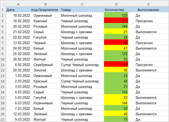
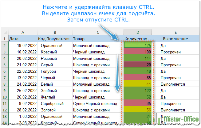
Предположим, у вас есть таблица со списком заказов, в которой ячейки в столбце «Количество» окрашены в зависимости от их значения в колонке «Выполнение» и даты: ячейки с выполняемыми заказами сроком до 30 дней от текущей даты — желтые, уже выполненные — зеленые, а просроченные заказы — красные.
Теперь нам нужно автоматически подсчитать ячейки определенного цвета, т.е. посчитать количество красных, зеленых и желтых ячеек в таблице. Как я объяснил выше, прямого решения этой задачи при помощи стандартных формул Excel не существует. Но, к счастью, есть код VBA для Excel. Выполните 5 быстрых шагов ниже, и вы узнаете число и сумму ваших цветных ячеек всего за несколько минут.
- Откройте книгу Excel и нажмите
Alt+F11, чтобы открыть редактор Visual Basic (VBE). - Щелкните правой кнопкой мыши имя своей книги в разделе «Project–VBAProject» в правой части экрана, а затем выберите «Вставить» > «Модуль» в контекстном меню.

- Добавьте в вашу рабочую книгу следующий код:
Function GetCellColor(xlRange As Range)
  Dim indRow, indColumn As Long
  Dim arResults()
  Dim colorVal As Variant

  Application.Volatile

  If xlRange Is Nothing Then
      Set xlRange = Application.ThisCell
  End If

  If xlRange.Count > 1 Then
    ReDim arResults(1 To xlRange.Rows.Count, 1 To xlRange.Columns.Count)
     For indRow = 1 To xlRange.Rows.Count
       For indColumn = 1 To xlRange.Columns.Count
         colorVal = xlRange(indRow, indColumn).Interior.Color
         arResults(indRow, indColumn) = (colorVal Mod 256) & ", " & ((colorVal  256) Mod 256) & ", " & (colorVal  65536)
       Next
     Next
   GetCellColor = arResults
  Else
   colorVal = xlRange.Cells(1, 1).Interior.Color
   GetCellColor = (colorVal Mod 256) & ", " & ((colorVal  256) Mod 256) & ", " & (colorVal  65536)
  End If
End Function

Function GetCellFontColor(xlRange As Range)
  Dim indRow, indColumn As Long
  Dim arResults()
  Dim colorVal As Variant

  Application.Volatile

  If xlRange Is Nothing Then
      Set xlRange = Application.ThisCell
  End If

  If xlRange.Count > 1 Then
    ReDim arResults(1 To xlRange.Rows.Count, 1 To xlRange.Columns.Count)
     For indRow = 1 To xlRange.Rows.Count
       For indColumn = 1 To xlRange.Columns.Count
         colorVal = xlRange(indRow, indColumn).Font.Color
         arResults(indRow, indColumn) = (colorVal Mod 256) & ", " & ((colorVal  256) Mod 256) & ", " & (colorVal  65536)
       Next
     Next
   GetCellFontColor = arResults
  Else
   colorVal = xlRange.Cells(1, 1).Font.Color
   GetCellFontColor = (colorVal Mod 256) & ", " & ((colorVal  256) Mod 256) & ", " & (colorVal  65536)
  End If
End Function

Function CountCellsByColor(rData As Range, cellRefColor As Range) As Long
    Dim indRefColor As Long
    Dim cellCurrent As Range
    Dim cntRes As Long

    Application.Volatile
    cntRes = 0
    indRefColor = cellRefColor.Cells(1, 1).Interior.Color
    For Each cellCurrent In rData
        If indRefColor = cellCurrent.Interior.Color Then
            cntRes = cntRes + 1
        End If
    Next cellCurrent

    CountCellsByColor = cntRes
End Function

Function SumCellsByColor(rData As Range, cellRefColor As Range)
    Dim indRefColor As Long
    Dim cellCurrent As Range
    Dim sumRes

    Application.Volatile
    sumRes = 0
    indRefColor = cellRefColor.Cells(1, 1).Interior.Color
    For Each cellCurrent In rData
        If indRefColor = cellCurrent.Interior.Color Then
            sumRes = WorksheetFunction.Sum(cellCurrent, sumRes)
        End If
    Next cellCurrent

    SumCellsByColor = sumRes
End Function

Function CountCellsByFontColor(rData As Range, cellRefColor As Range) As Long
    Dim indRefColor As Long
    Dim cellCurrent As Range
    Dim cntRes As Long

    Application.Volatile
    cntRes = 0
    indRefColor = cellRefColor.Cells(1, 1).Font.Color
    For Each cellCurrent In rData
        If indRefColor = cellCurrent.Font.Color Then
            cntRes = cntRes + 1
        End If
    Next cellCurrent

    CountCellsByFontColor = cntRes
End Function

Function SumCellsByFontColor(rData As Range, cellRefColor As Range)
    Dim indRefColor As Long
    Dim cellCurrent As Range
    Dim sumRes

    Application.Volatile
    sumRes = 0
    indRefColor = cellRefColor.Cells(1, 1).Font.Color
    For Each cellCurrent In rData
        If indRefColor = cellCurrent.Font.Color Then
            sumRes = WorksheetFunction.Sum(cellCurrent, sumRes)
        End If
    Next cellCurrent

    SumCellsByFontColor = sumRes
End Function- Сохраните свою книгу как «Книга Excel с поддержкой макросов (.xlsm)».
Если вы новичок и вам сложно работать с VBA, вы можете найти подробные пошаговые инструкции и несколько полезных советов в этом руководстве: Как вставить и запустить код VBA в Excel .
- Теперь, когда вся подготовительная работа сделана, выберите ячейку, в которой вы хотите получить результат, и введите в нее только что записанную нами пользовательскую функцию CountCellsByColor:
CountCellsByColor( диапазон ; код цвета )
здесь и далее эти аргументы означают:
диапазон – диапазон ячеек, в которых вы хотите произвести подсчеты по цвету,
код цвета – адрес ячейки-образца, цвет фона или шрифта которой соответствуют искомому цвету фона или шрифта.
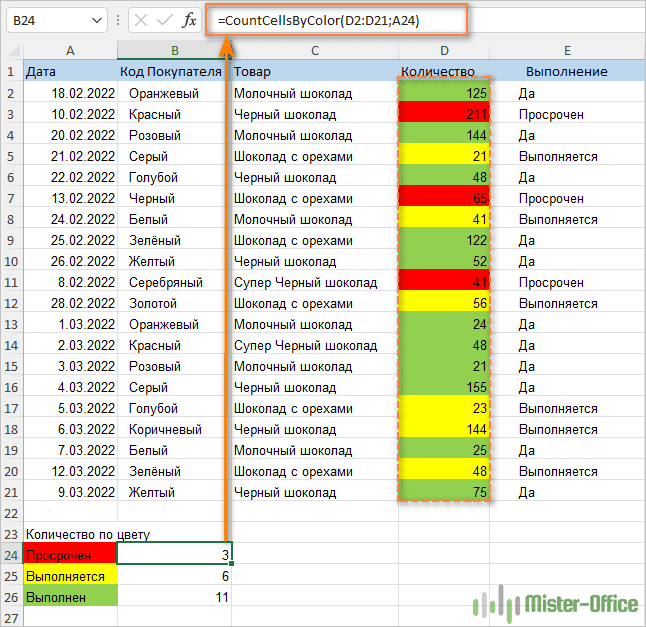
В этом примере мы используем формулу, =CountCellsByColor(D2:D21;A24), где D2:D21— это диапазон, в котором вы хотите посчитать количество ячеек с цветом, а A24 — это ячейка, закрашенная нужным нам цветом, красным в нашем случае.
Аналогичным образом вы записываете формулы для других цветов, которые хотите посчитать, желтого и зеленого, в нашей таблице.
Если у вас есть числовые данные в цветных ячейках (например, столбец Количество в нашей таблице), вы можете сложить значения на основе определенного цвета, используя аналогичную функцию SumCellsByColor:
SumCellsByColor( диапазон ; код цвета)

Как показано на скриншоте выше, мы использовали формулу суммы по цвету, =SumCellsByColor(D2:D21;A24), где D2:D21 — это диапазон, а A24 — ячейка с образцом цвета.
Аналогичным образом вы можете посчитать выделенные цветом ячейки и суммировать значения таких ячеек по цвету шрифта, используя функции CountCellsByFontColor и SumCellsByFontColor соответственно.
На скриншоте ниже вы видите, как можно подсчитать количество значений, написанных красным цветом.
=CountCellsByFontColor(D2:D21;A24)

Аналогично подсчитываем сумму чисел, имеющих определённый цвет шрифта, при помощи формулы:
=SumCellsByFontColor(D2:D21;A24)

Примечание. Если после применения вышеупомянутого кода VBA вам потребуется раскрасить еще несколько ячеек вручную, то сумма и количество окрашенных ячеек не будут пересчитаны автоматически, чтобы отразить произошедшие изменения. Пожалуйста, не сердитесь на нас, это не ошибка кода 
На самом деле, это нормальное поведение всех макросов Excel, скриптов VBA и пользовательских функций. Дело в том, что все подобные функции вызываются только при изменении данных рабочего листа. Но Excel не воспринимает изменение цвета шрифта или цвета ячейки как изменение данных.
Итак, после раскрашивания ячеек вручную, просто поместите курсор в любую ячейку и нажмите F2, а затем Enter. То есть, сделайте вид, что меняете содержимое какой-либо ячейки. Сумма и количество в пользовательской функции тут же будут обновлены. То же самое относится и к другим макросам, которые считают по цвету.
Как суммировать по цвету и сосчитать по цвету во всей рабочей книге
Приведенная ниже пользовательская функция подсчитывает и находит сумму ячеек по цвету заливки на всех листах рабочей книги. Итак, вот ее код:
Function WbkCountCellsByColor(cellRefColor As Range)
  Dim vWbkRes
  Dim wshCurrent As Worksheet

  Application.ScreenUpdating = False
  Application.Calculation = xlCalculationManual

  vWbkRes = 0
  For Each wshCurrent In Worksheets
    wshCurrent.Activate
    vWbkRes = vWbkRes + CountCellsByColor(wshCurrent.UsedRange, cellRefColor)
  Next
  Application.ScreenUpdating = True
  Application.Calculation = xlCalculationAutomatic

  WbkCountCellsByColor = vWbkRes
End Function

Function WbkSumCellsByColor(cellRefColor As Range)
  Dim vWbkRes
  Dim wshCurrent As Worksheet

  Application.ScreenUpdating = False
  Application.Calculation = xlCalculationManual

  vWbkRes = 0
  For Each wshCurrent In Worksheets
    wshCurrent.Activate
    vWbkRes = vWbkRes + SumCellsByColor(wshCurrent.UsedRange, cellRefColor)
  Next
  Application.ScreenUpdating = True
  Application.Calculation = xlCalculationAutomatic

  WbkSumCellsByColor = vWbkRes
End Function
Вы используете этот макрос так же, как и предыдущий код, и выводите количество и сумму цветных ячеек с помощью следующих формул =WbkCountCellsByColor() и =WbkSumCellsByColor() соответственно.
Единственный аргумент, который нужен этим функциям, это адрес ячейки с нужным цветом.
Просто введите любую из этих формул в любую пустую ячейку на любом листе без указания диапазона, используйте в скобках адрес ячейки нужного цвета, например
=WbkSumCellsByColor(A1)
Формула отобразит сумму всех ячеек, закрашенных тем же цветом, на всех листах в вашей рабочей книге.
Пользовательские функции для получения цвета ячейки, цвета шрифта и цветового кода
Здесь вы найдете перечень всех функций, которые мы использовали ранее, а также несколько новых, которые извлекают цветовые коды.
Зачем они нам? Но ведь если ваша таблица окрашена не совсем стандартными цветами (например, светло-зеленым), то подобрать образец цвета для функций, которые мы рассматривали выше, будет весьма затруднительно. Если же у вас будет код нужного цвета, вы сможете использовать его при форматировании ячейки-образца, чтобы получить точное соответствие цвета.
Если вы вдруг забыли, как можно вручную раскрасить ячейку в нужный цвет, то напомню. Жмем Ctrl+1, затем Заливка – Другие цвета – Спектр – RGB формат. Вот туда и вставляем полученный код. Точное соответствие цвета будет обеспечено.
Примечание. Помните, что все эти формулы будут работать только в том случае, если вы добавили пользовательскую функцию в книгу Excel, как показано ранее в этой статье.
Функции для подсчета по цвету:
- CountCellsByColor(диапазон; код цвета) – считает ячейки с заданным цветом фона.
В приведенном выше примере мы использовали следующую формулу для подсчета ячеек по цвету
= CountCellsByColor (F2: F14, A17)
где F2: F14 — выбранный диапазон, а A17 — ячейка с нужным цветом фона. Вы можете использовать все остальные формулы, перечисленные ниже, аналогичным образом.
- CountCellsByFontColor(диапазон; код цвета) – подсчитывает ячейки с указанным цветом шрифта.
Формулы для суммирования по цветам:
- SumCellsByColor(диапазон; код цвета) – вычисляет сумму ячеек с определенным цветом фона.
- SumCellsByFontColor(диапазон; код цвета) – вычисляет сумму ячеек с определенным цветом шрифта.
Функции для получения кода цвета ячейки:
- GetCellFontColor(ячейка) – возвращает цветовой код цвета шрифта указанной ячейки.
- GetCellColor(ячейка) – возвращает цветовой код цвета фона указанной ячейки.
Вот примеры использования функции цвета ячейки:

А на этим скриншоте мы получаем цветовой RGB код шрифта.

Как считать по цвету и суммировать ячейки, окрашенные с использованием условного форматирования
Если вы применили условное форматирование к ячейкам на основе их значений и теперь хотите посчитать эти ячейки по цвету или просуммировать значения в закрашенных ячейках, то у меня плохие новости — не существует универсальной определяемой пользователем функции, которая бы суммировала по цвету или пересчитала закрашенные условным форматированием ячейки и вывела бы полученные числа прямо в указанные клетки таблицы. По крайней мере мне о такой функции не известно, увы 
Конечно, вы можете найти в Интернете тонны кода VBA, который пытается это сделать, но все эти коды (по крайней мере, примеры, с которыми я сталкивался), не обрабатывают условное форматирование, такое как «Форматировать все ячейки на основе их значений», «Форматировать только наибольшие или наименьшие значения», «Форматировать только значения выше или ниже среднего», «Форматировать только уникальные или повторяющиеся значения». Кроме того, почти все эти коды VBA имеют ряд особенностей и ограничений, из-за которых они могут работать некорректно с определенными книгами или типами данных. В общем, вы можете испытать удачу и поискать в Google идеальное решение, и если вы его найдете, пожалуйста, вернитесь и опубликуйте свое открытие здесь!
Но если пользовательская функция не может выполнить эту задачу, то макрос VBA вполне может справиться. О различиях пользовательских функций и макросов VBA вы можете более подробно прочитать в этой статье.
Приведенный ниже макрос VBA преодолевает вышеупомянутые ограничения и работает в электронных таблицах Microsoft Excel со всеми типами условного форматирования. Он отображает количество выделенных определенным цветом ячеек и сумму значений в этих ячейках, независимо от того, какой тип условного форматирования используется на листе.
Sub SumCountByConditionalFormat()
  Dim indRefColor As Long
  Dim cellCurrent As Object
  Dim cntRes As Long
  Dim sumRes
  Dim cntCells As Long
  Dim indCurCell As Long

  cntRes = 0
  sumRes = 0

  Set cellCurrent = Selection
  adr = Mid(cellCurrent.Address, InStr(cellCurrent.Address, ",") + 1, 20)
  adr1 = Left(adr, 4)
  adr2 = Left(cellCurrent.Address, InStr(cellCurrent.Address, ",") - 1)
  Range(adr2).Activate
  indRefColor = ActiveCell.DisplayFormat.Interior.Color
  Range(adr).Activate
  cntCells = Selection.CountLarge
  Range(adr).Select
  Range(adr).Activate
 Set cellCurrent = Selection
 For indCurCell = 1 To (cntCells - 1)
    If indRefColor = cellCurrent(indCurCell).DisplayFormat.Interior.Color Then
        cntRes = cntRes + 1
        sumRes = WorksheetFunction.Sum(cellCurrent(indCurCell), sumRes)
    End If
  Next
  MsgBox "Count=" & cntRes & vbCrLf & "Sum= " & sumRes & vbCrLf & vbCrLf & _
    "Color=" & Left("000000", 6 - Len(Hex(indRefColor))) & _
    Hex(indRefColor) & vbCrLf, , "Count & Sum by Conditional Format color"
End Sub
Как использовать этот макрос для подсчета цветных ячеек и суммирования их значений.
Опишем процесс пошагово:
- Добавьте приведенный выше код на лист, как описано в первом параграфе статьи .
- Выберите ячейку с нужным цветом.
- Нажмите и удерживайте
Ctrl. - Выберите диапазон, в котором вы хотите подсчитать цветные ячейки и/или суммировать по цвету, если у вас есть числовые данные.
- Отпустите клавишу
Ctrl. - НажНажмите комбинацию
Alt+F8, чтобы открыть список макросов в вашей книге. - Выберите макрос SumCountByConditionalFormat и нажмите «Выполнить» .
Покажем эти действия на скриншотах. Используем пример данных, с которыми мы уже работали в первых параграфах этой статьи. Только теперь они окрашены в столбце В при помощи условного форматирования.
Сначала выбираем ячейку D5, поскольку хотим подсчитать ячейки красного цвета с просроченными заказами.

Затем дополнительно, удерживая Ctrl, выделяем диапазон ячеек в столбце D, по которым нужно выполнить подсчет ячеек определенного цвета.
Выполняем макрос, как показано на скриншоте ниже.

В результате вы увидите следующее сообщение с результатами:

Для этого примера мы выбрали столбец «Количество» и получили следующие цифры:
- Count — это количество ячеек определенного цвета, красного в нашем случае, который отмечает ячейки «Просрочен».
- Sum — это сумма значений всех красных ячеек в выбранной колонке, т.е. общее количество «Просроченных» заказов.
- Color — это шестнадцатеричный код цвета выбранной ячейки, в нашем случае D5.
Таким образом мы можем посчитать сумму и количество по цвету ячеек с условным форматированием.
Самый быстрый способ подсчета и суммирования ячеек по цвету в Excel
Я могу рекомендовать вам надстройку для Excel, которая бы считала и суммировала ячейки по указанному вами цвету или по всем цветам в выбранном диапазоне.
При этом не имеет значения, как установлены эти цвета – прямым форматированием ячейки либо при помощи условного форматирования.
Позвольте представить вам наш совершенно новый инструмент — «Счет и сумма по цвету» для Excel. Он имеет два варианта подсчета — «Один цвет» и «Все цвета», как видно на скриншоте ниже.
Подсчет и суммирование по одному цвету.
Вы нажимаете кнопку « Один цвет » на ленте, и в левой части рабочего листа открывается панель « Подсчет и сумма по цвету» . На панели вы выбираете:
- Диапазон, в котором вы хотите подсчитать и суммировать ячейки
- Любую ячейку с нужным цветом как образец
- Вариант — цвет фона или шрифта
После этого нажмите « Рассчитать » и сразу же увидите результат в нижней части панели! Помимо подсчета и суммы, надстройка вычисляет среднее значение и находит максимальное и минимальное значения. Никаких макросов, никаких формул, никакой боли
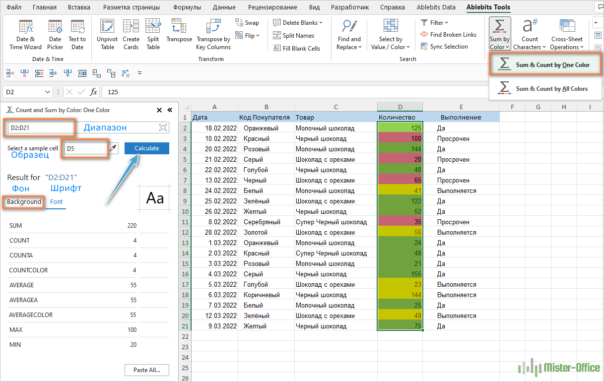
Обратите внимание, что подсчет возможен как по цвету фона, так и по цвету шрифта.
Подсчет и суммирование ячеек по всем цветам в выбранном диапазоне
Опция «Все цвета» работает в основном так же, за исключением того, что вам не нужно выбирать цвет. В разделе «Result for ..» вы можете выбрать любой из параметров: Количество, Сумма, Среднее, Максимальное или Минимальное значение и другие.
Если вы хотите скопировать результаты на свой рабочий лист, нажмите кнопку «Paste All…» в нижней части панели .

В настоящее время надстройка доступна как часть Ultimate Suite for Excel . Это коллекция отличных инструментов, специально разработанных для решения самых утомительных, кропотливых и подверженных ошибкам задач в Excel.
В дополнение к надстройке «Подсчет и суммирование по цвету», Ultimate Suite включает более 70 инструментов, которые помогут вам объединить данные из разных листов, удалить дубликаты, сравнить листы на совпадения и различия и многое другое.
Надеюсь, теперь сумма по цвету и подсчет ячеек по цвету для вас не будут сложными. Если же будут вопросы – не стесняйтесь задавать их в комментариях.
 Функция СУММПРОИЗВ с примерами формул — В статье объясняются основные и расширенные способы использования функции СУММПРОИЗВ в Excel. Вы найдете ряд примеров формул для сравнения массивов, условного суммирования и подсчета ячеек по нескольким условиям, расчета средневзвешенного значения…
  Проверка данных с помощью регулярных выражений — В этом руководстве показано, как выполнять проверку данных в Excel с помощью регулярных выражений и пользовательской функции RegexMatch. Когда дело доходит до ограничения пользовательского ввода на листах Excel, проверка данных очень полезна. Хотите… Поиск и замена в Excel с помощью регулярных выражений — В этом руководстве показано, как быстро добавить пользовательскую функцию в свои рабочие книги, чтобы вы могли использовать регулярные выражения для замены текстовых строк в Excel. Когда дело доходит до замены… Как извлечь строку из текста при помощи регулярных выражений — В этом руководстве вы узнаете, как использовать регулярные выражения в Excel для поиска и извлечения части текста, соответствующего заданному шаблону. Microsoft Excel предоставляет ряд функций для извлечения текста из ячеек. Эти функции…
  4 способа отладки пользовательской функции — Как правильно создавать пользовательские функции и где нужно размещать их код, мы подробно рассмотрели ранее в этой статье. Чтобы решить проблемы при создании пользовательской функции, вам скорее всего придется выполнить…
Often you may want to sum values in Excel based on their color.
For example, suppose we have the following dataset and we’d like to sum the values in the cells based on the cell colors:

The easiest way to do this is by writing some code in VBA in Excel.
This might seem intimidating if you’re not familiar with VBA but the process is straightforward and the following step-by-step example shows exactly how to do so.
Step 1: Enter the Data
First, enter the data values into Excel:
Step 2: Show the Developer Tab in Excel
Next, we need to make sure the Developer tab is visible on the top ribbon in Excel.
To do so, click the File tab, then click Options, then click Customize Ribbon.
Under the section called Main Tabs, check the box next to Developer, then click OK:

Step 3: Create a Macro Using VBA
Next, click the Developer tab along the top ribbon and then click the Visual Basic icon:

Next, click the Insert tab and then click Module from the dropdown menu:

Next, paste the following code into the module code editor:
Function SumCellsByColor(CellRange As Range, CellColor As Range)

Dim CellColorValue As Integer
Dim RunningSum As Long

CellColorValue = CellColor.Interior.ColorIndex
Set i = CellRange

For Each i In CellRange
    If i.Interior.ColorIndex = CellColorValue Then
    RunningSum = RunningSum + i.Value
    End If
Next i

SumCellsByColor = RunningSum

End Function
The following screenshot shows how to do so:

Next, close the VB Editor.
Step 4: Use the Macro to Sum Cells by Color
Lastly, we can use the macro we created to sum the cells based on color.
First, fill in cells C2:C4 with the colors that you’d like to sum.
Then type the following formula into cell D2:
=SumCellsByColor($A$2:$A$11, C2)
Drag and fill this formula down to each remaining cell in column D and the formula will automatically sum each of the cells that have specific background colors:

For example, we can see that the sum of the cells with a light green background is 53.
We can confirm this by manually calculating the sum of each cell with a light green background:
Sum of Cells with Light Green Background: 20 + 13 + 20 = 53.
This matches the value calculated by our formula.
Additional Resources
The following tutorials explain how to perform other common tasks in Excel:
How to Sum by Category in Excel
How to Sum by Year in Excel
How to Sum by Month in Excel
How to Sum by Week in Excel