
SEARCH, SEARCHB functions
Excel for Microsoft 365 Excel for Microsoft 365 for Mac Excel for the web Excel 2021 Excel 2021 for Mac Excel 2019 Excel 2019 for Mac Excel 2016 Excel 2016 for Mac Excel 2013 Excel 2010 Excel 2007 Excel for Mac 2011 Excel Starter 2010 More…Less
This article describes the formula syntax and usage of the SEARCH and SEARCHB functions in Microsoft Excel.
Description
The SEARCH and SEARCHB functions locate one text string within a second text string, and return the number of the starting position of the first text string from the first character of the second text string. For example, to find the position of the letter «n» in the word «printer», you can use the following function:
=SEARCH(«n»,»printer»)
This function returns 4 because «n» is the fourth character in the word «printer.»
You can also search for words within other words. For example, the function
=SEARCH(«base»,»database»)
returns 5, because the word «base» begins at the fifth character of the word «database». You can use the SEARCH and SEARCHB functions to determine the location of a character or text string within another text string, and then use the MID and MIDB functions to return the text, or use the REPLACE and REPLACEB functions to change the text. These functions are demonstrated in Example 1 in this article.
Important:
-
These functions may not be available in all languages.
-
SEARCHB counts 2 bytes per character only when a DBCS language is set as the default language. Otherwise SEARCHB behaves the same as SEARCH, counting 1 byte per character.
The languages that support DBCS include Japanese, Chinese (Simplified), Chinese (Traditional), and Korean.
Syntax
SEARCH(find_text,within_text,[start_num])
SEARCHB(find_text,within_text,[start_num])
The SEARCH and SEARCHB functions have the following arguments:
-
find_text Required. The text that you want to find.
-
within_text Required. The text in which you want to search for the value of the find_text argument.
-
start_num Optional. The character number in the within_text argument at which you want to start searching.
Remark
-
The SEARCH and SEARCHB functions are not case sensitive. If you want to do a case sensitive search, you can use FIND and FINDB.
-
You can use the wildcard characters — the question mark (?) and asterisk (*) — in the find_text argument. A question mark matches any single character; an asterisk matches any sequence of characters. If you want to find an actual question mark or asterisk, type a tilde (~) before the character.
-
If the value of find_text is not found, the #VALUE! error value is returned.
-
If the start_num argument is omitted, it is assumed to be 1.
-
If start_num is not greater than 0 (zero) or is greater than the length of the within_text argument, the #VALUE! error value is returned.
-
Use start_num to skip a specified number of characters. Using the SEARCH function as an example, suppose you are working with the text string «AYF0093.YoungMensApparel». To find the position of the first «Y» in the descriptive part of the text string, set start_num equal to 8 so that the serial number portion of the text (in this case, «AYF0093») is not searched. The SEARCH function starts the search operation at the eighth character position, finds the character that is specified in the find_text argument at the next position, and returns the number 9. The SEARCH function always returns the number of characters from the start of the within_text argument, counting the characters you skip if the start_num argument is greater than 1.
Examples
Copy the example data in the following table, and paste it in cell A1 of a new Excel worksheet. For formulas to show results, select them, press F2, and then press Enter. If you need to, you can adjust the column widths to see all the data.
|
Data |
||
|---|---|---|
|
Statements |
||
|
Profit Margin |
||
|
margin |
||
|
The «boss» is here. |
||
|
Formula |
Description |
Result |
|
=SEARCH(«e»,A2,6) |
Position of the first «e» in the string in cell A2, starting at the sixth position. |
7 |
|
=SEARCH(A4,A3) |
Position of «margin» (string for which to search is cell A4) in «Profit Margin» (cell in which to search is A3). |
8 |
|
=REPLACE(A3,SEARCH(A4,A3),6,»Amount») |
Replaces «Margin» with «Amount» by first searching for the position of «Margin» in cell A3, and then replacing that character and the next five characters with the string «Amount.» |
Profit Amount |
|
=MID(A3,SEARCH(» «,A3)+1,4) |
Returns the first four characters that follow the first space character in «Profit Margin» (cell A3). |
Marg |
|
=SEARCH(«»»»,A5) |
Position of the first double quotation mark («) in cell A5. |
5 |
|
=MID(A5,SEARCH(«»»»,A5)+1,SEARCH(«»»»,A5,SEARCH(«»»»,A5)+1)-SEARCH(«»»»,A5)-1) |
Returns only the text enclosed in the double quotation marks in cell A5. |
boss |
Need more help?
Want more options?
Explore subscription benefits, browse training courses, learn how to secure your device, and more.
Communities help you ask and answer questions, give feedback, and hear from experts with rich knowledge.
![]()
Download Article
![]()
Download Article
An Excel document can be overwhelming to look through. Thankfully, you can use the search function to conveniently locate a particular word, or group of words, in an Excel worksheet.
-

1
Launch MS Excel. Do this by clicking on its icon in your desktop. It is the green X icon with spreadsheets in its background.
- If you don’t have an Excel shortcut icon on your desktop, find it in your Start menu and click the icon there.
-
2
Find the Excel file you want to open. Click “File” in the upper left corner of the window then click “Open.” A file browser will appear. Browse your computer for the Excel file you want to open.
Advertisement
-
3
Open the file. Once you’ve located the file, click on it to select then click “Open” in the lower-right portion of the file browser.


Advertisement
-
1
Click a cell. Once you’re in the worksheet, click on any cell on the worksheet to ensure that the window is active.
-
2
Open the Find/Replace With window. Hit the key combination Ctrl + F on your keyboard. A new window will appear with two fields: “Find” and “Replace with.”
-
3
Type in the words you want to find. Enter the exact word or phrase you want to search for, and click on the “Find” button in the lower right of the Find window.
- Excel will begin searching for matches of the word, or words, you entered in the search field. All words in the document that matches those you entered will be highlighted to help you better locate them.


Advertisement
Ask a Question
200 characters left
Include your email address to get a message when this question is answered.
Submit
Advertisement
Thanks for submitting a tip for review!
About This Article
Thanks to all authors for creating a page that has been read 91,003 times.
Is this article up to date?
Содержание
- Поисковая функция в Excel
- Способ 1: простой поиск
- Способ 2: поиск по указанному интервалу ячеек
- Способ 3: Расширенный поиск
- Вопросы и ответы

В документах Microsoft Excel, которые состоят из большого количества полей, часто требуется найти определенные данные, наименование строки, и т.д. Очень неудобно, когда приходится просматривать огромное количество строк, чтобы найти нужное слово или выражение. Сэкономить время и нервы поможет встроенный поиск Microsoft Excel. Давайте разберемся, как он работает, и как им пользоваться.
Поисковая функция в Excel
Поисковая функция в программе Microsoft Excel предлагает возможность найти нужные текстовые или числовые значения через окно «Найти и заменить». Кроме того, в приложении имеется возможность расширенного поиска данных.
Способ 1: простой поиск
Простой поиск данных в программе Excel позволяет найти все ячейки, в которых содержится введенный в поисковое окно набор символов (буквы, цифры, слова, и т.д.) без учета регистра.
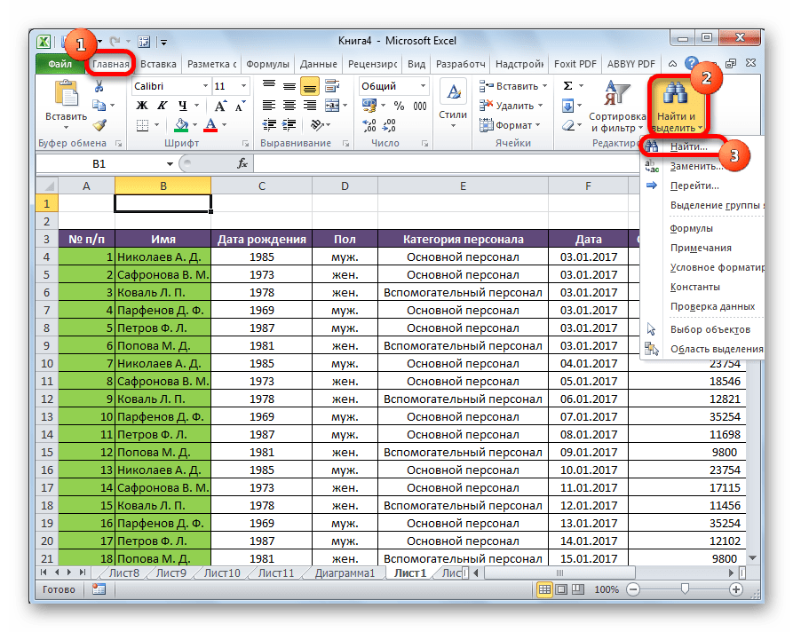
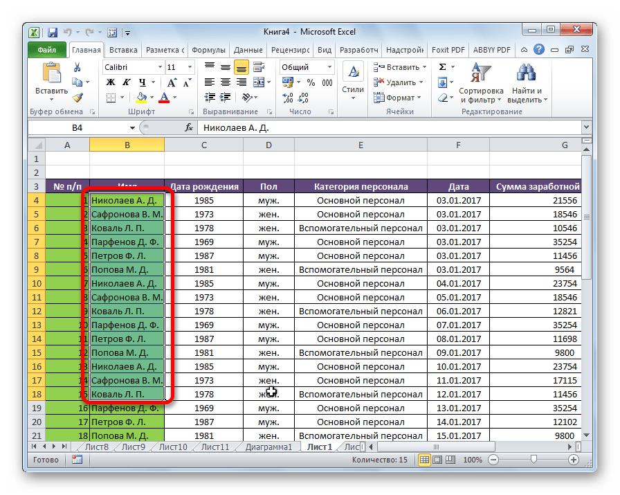
- Находясь во вкладке «Главная», кликаем по кнопке «Найти и выделить», которая расположена на ленте в блоке инструментов «Редактирование». В появившемся меню выбираем пункт «Найти…». Вместо этих действий можно просто набрать на клавиатуре сочетание клавиш Ctrl+F.
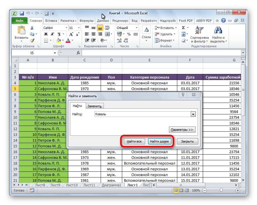
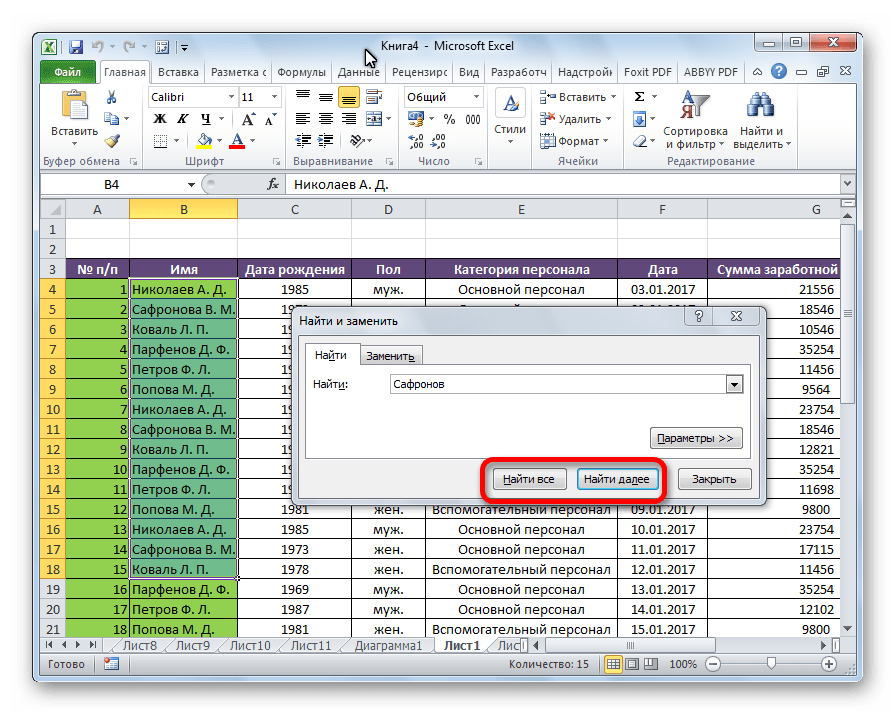
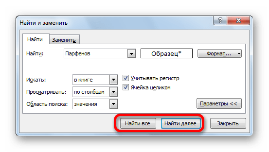
- После того, как вы перешли по соответствующим пунктам на ленте, или нажали комбинацию «горячих клавиш», откроется окно «Найти и заменить» во вкладке «Найти». Она нам и нужна. В поле «Найти» вводим слово, символы, или выражения, по которым собираемся производить поиск. Жмем на кнопку «Найти далее», или на кнопку «Найти всё».
- При нажатии на кнопку «Найти далее» мы перемещаемся к первой же ячейке, где содержатся введенные группы символов. Сама ячейка становится активной.
Поиск и выдача результатов производится построчно. Сначала обрабатываются все ячейки первой строки. Если данные отвечающие условию найдены не были, программа начинает искать во второй строке, и так далее, пока не отыщет удовлетворительный результат.
Поисковые символы не обязательно должны быть самостоятельными элементами. Так, если в качестве запроса будет задано выражение «прав», то в выдаче будут представлены все ячейки, которые содержат данный последовательный набор символов даже внутри слова. Например, релевантным запросу в этом случае будет считаться слово «Направо». Если вы зададите в поисковике цифру «1», то в ответ попадут ячейки, которые содержат, например, число «516».
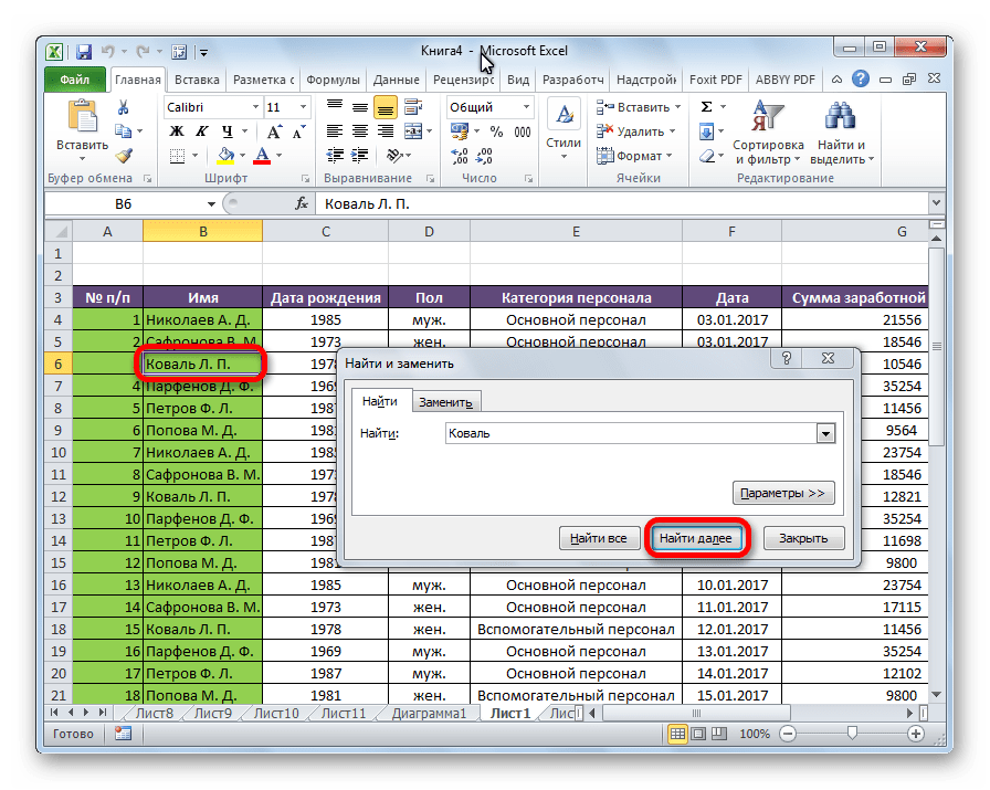
Для того, чтобы перейти к следующему результату, опять нажмите кнопку «Найти далее».

Так можно продолжать до тех, пор, пока отображение результатов не начнется по новому кругу.
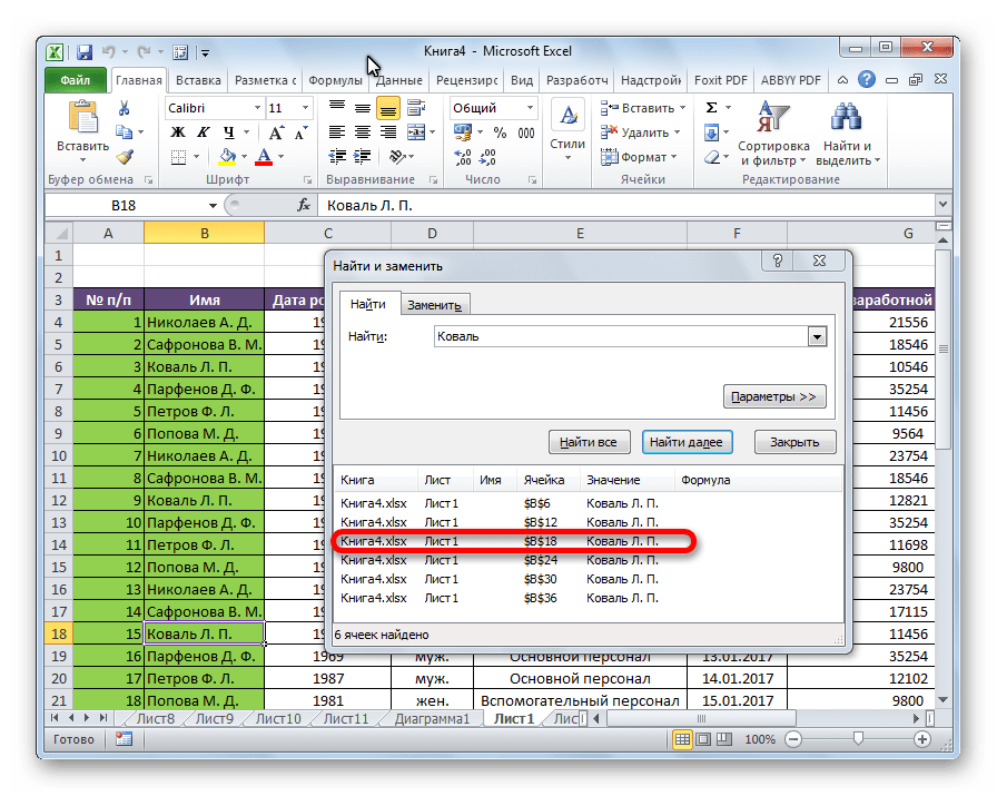
- В случае, если при запуске поисковой процедуры вы нажмете на кнопку «Найти все», все результаты выдачи будут представлены в виде списка в нижней части поискового окна. В этом списке находятся информация о содержимом ячеек с данными, удовлетворяющими запросу поиска, указан их адрес расположения, а также лист и книга, к которым они относятся. Для того, чтобы перейти к любому из результатов выдачи, достаточно просто кликнуть по нему левой кнопкой мыши. После этого курсор перейдет на ту ячейку Excel, по записи которой пользователь сделал щелчок.
Способ 2: поиск по указанному интервалу ячеек
Если у вас довольно масштабная таблица, то в таком случае не всегда удобно производить поиск по всему листу, ведь в поисковой выдаче может оказаться огромное количество результатов, которые в конкретном случае не нужны. Существует способ ограничить поисковое пространство только определенным диапазоном ячеек.
- Выделяем область ячеек, в которой хотим произвести поиск.
- Набираем на клавиатуре комбинацию клавиш Ctrl+F, после чего запуститься знакомое нам уже окно «Найти и заменить». Дальнейшие действия точно такие же, что и при предыдущем способе. Единственное отличие будет состоять в том, что поиск выполняется только в указанном интервале ячеек.
Способ 3: Расширенный поиск
Как уже говорилось выше, при обычном поиске в результаты выдачи попадают абсолютно все ячейки, содержащие последовательный набор поисковых символов в любом виде не зависимо от регистра.

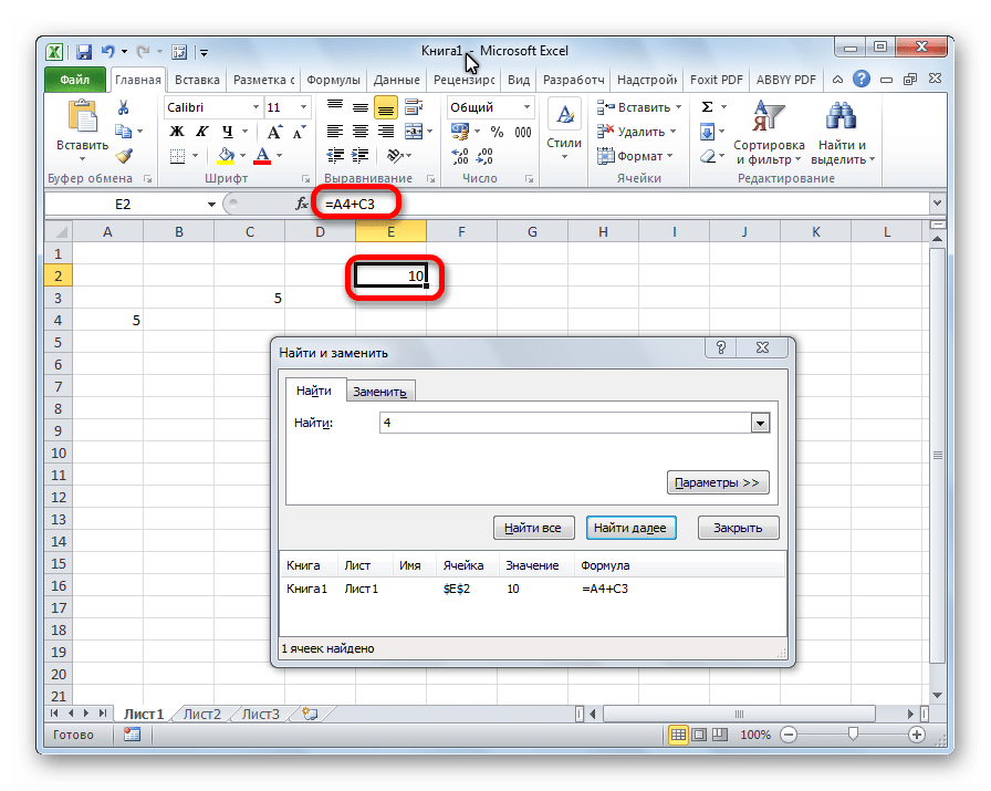
К тому же, в выдачу может попасть не только содержимое конкретной ячейки, но и адрес элемента, на который она ссылается. Например, в ячейке E2 содержится формула, которая представляет собой сумму ячеек A4 и C3. Эта сумма равна 10, и именно это число отображается в ячейке E2. Но, если мы зададим в поиске цифру «4», то среди результатов выдачи будет все та же ячейка E2. Как такое могло получиться? Просто в ячейке E2 в качестве формулы содержится адрес на ячейку A4, который как раз включает в себя искомую цифру 4.
Но, как отсечь такие, и другие заведомо неприемлемые результаты выдачи поиска? Именно для этих целей существует расширенный поиск Excel.
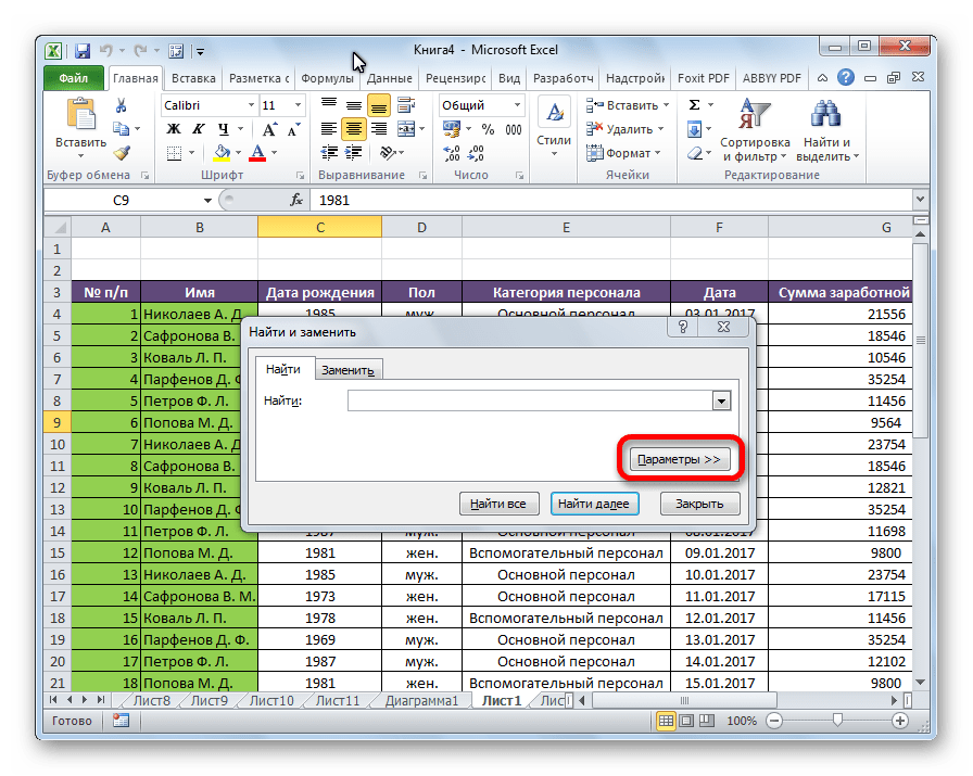
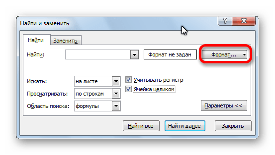
- После открытия окна «Найти и заменить» любым вышеописанным способом, жмем на кнопку «Параметры».
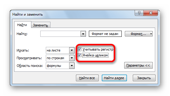
- В окне появляется целый ряд дополнительных инструментов для управления поиском. По умолчанию все эти инструменты находятся в состоянии, как при обычном поиске, но при необходимости можно выполнить корректировку.

По умолчанию, функции «Учитывать регистр» и «Ячейки целиком» отключены, но, если мы поставим галочки около соответствующих пунктов, то в таком случае, при формировании результата будет учитываться введенный регистр, и точное совпадение. Если вы введете слово с маленькой буквы, то в поисковую выдачу, ячейки содержащие написание этого слова с большой буквы, как это было бы по умолчанию, уже не попадут. Кроме того, если включена функция «Ячейки целиком», то в выдачу будут добавляться только элементы, содержащие точное наименование. Например, если вы зададите поисковый запрос «Николаев», то ячейки, содержащие текст «Николаев А. Д.», в выдачу уже добавлены не будут.
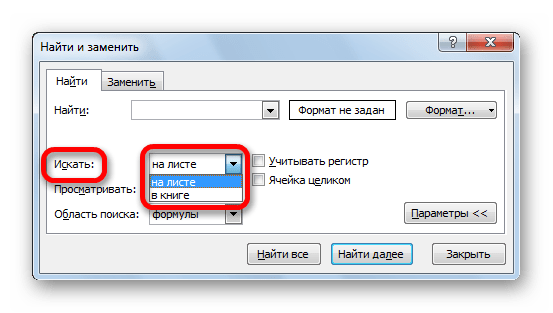
По умолчанию, поиск производится только на активном листе Excel. Но, если параметр «Искать» вы переведете в позицию «В книге», то поиск будет производиться по всем листам открытого файла.
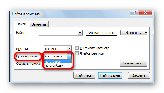
В параметре «Просматривать» можно изменить направление поиска. По умолчанию, как уже говорилось выше, поиск ведется по порядку построчно. Переставив переключатель в позицию «По столбцам», можно задать порядок формирования результатов выдачи, начиная с первого столбца.
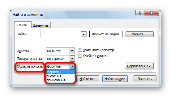
В графе «Область поиска» определяется, среди каких конкретно элементов производится поиск. По умолчанию, это формулы, то есть те данные, которые при клике по ячейке отображаются в строке формул. Это может быть слово, число или ссылка на ячейку. При этом, программа, выполняя поиск, видит только ссылку, а не результат. Об этом эффекте велась речь выше. Для того, чтобы производить поиск именно по результатам, по тем данным, которые отображаются в ячейке, а не в строке формул, нужно переставить переключатель из позиции «Формулы» в позицию «Значения». Кроме того, существует возможность поиска по примечаниям. В этом случае, переключатель переставляем в позицию «Примечания».
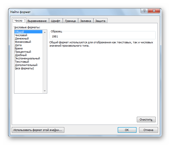
Ещё более точно поиск можно задать, нажав на кнопку «Формат».
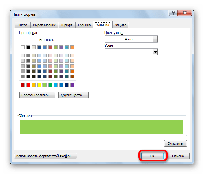
При этом открывается окно формата ячеек. Тут можно установить формат ячеек, которые будут участвовать в поиске. Можно устанавливать ограничения по числовому формату, по выравниванию, шрифту, границе, заливке и защите, по одному из этих параметров, или комбинируя их вместе.

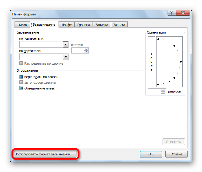
Если вы хотите использовать формат какой-то конкретной ячейки, то в нижней части окна нажмите на кнопку «Использовать формат этой ячейки…».
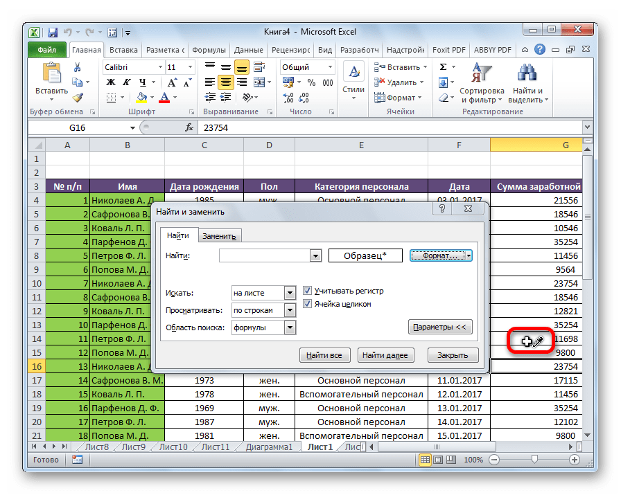
После этого, появляется инструмент в виде пипетки. С помощью него можно выделить ту ячейку, формат которой вы собираетесь использовать.
После того, как формат поиска настроен, жмем на кнопку «OK».
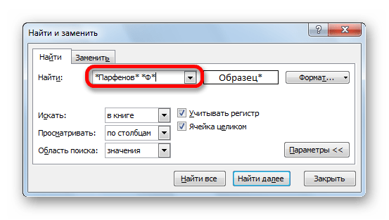
Бывают случаи, когда нужно произвести поиск не по конкретному словосочетанию, а найти ячейки, в которых находятся поисковые слова в любом порядке, даже, если их разделяют другие слова и символы. Тогда данные слова нужно выделить с обеих сторон знаком «*». Теперь в поисковой выдаче будут отображены все ячейки, в которых находятся данные слова в любом порядке.
- Как только настройки поиска установлены, следует нажать на кнопку «Найти всё» или «Найти далее», чтобы перейти к поисковой выдаче.

Как видим, программа Excel представляет собой довольно простой, но вместе с тем очень функциональный набор инструментов поиска. Для того, чтобы произвести простейший писк, достаточно вызвать поисковое окно, ввести в него запрос, и нажать на кнопку. Но, в то же время, существует возможность настройки индивидуального поиска с большим количеством различных параметров и дополнительных настроек.
Excel Search For Text (Table of Contents)
- Searching For Text in Excel
- How to Search Text in Excel?
Searching For Text in Excel
In excel, you might have seen situations where you want to extract the text present at a specific position in an entire string using text formulae such as LEFT, RIGHT, MID, etc. You can also use SEARCH and FIND functions in combination to find the text substring from a given string. However, when you are not interested in finding out the substring, but you want to find out whether a particular string is present in a given cell or not, not all of these formulae will work. In this article, we will go through some of the formulae and/or functions in Excel, which will allow you to check whether or not a particular string is present in a given cell.
How to Search Text in Excel?
Search For Text in Excel is very simple and easy. Let’s understand how to Search Text in Excel with some examples.
You can download this Search For Text Excel Template here – Search For Text Excel Template
Example #1 – Using Find Function
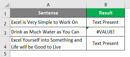
Let’s use the FIND function to find if a specific string is present in a cell or not. Suppose you have data as shown below.
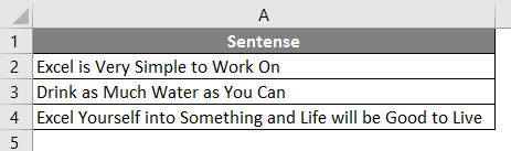
As we are trying to find whether a specific text is present in a given string or not, we have a function called FIND to deal with it on an initial level. This function returns a position of a substring in a text cell. Therefore, we can say that if the FIND function returns any numeric value, then the substring is present in the text else not.
Step 1: In cell B1, start typing =FIND; you will be able to access the function itself.
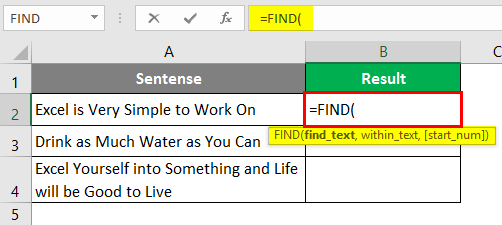
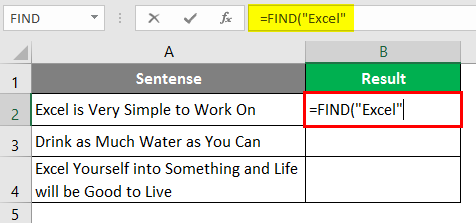
Step 2: The FIND function needs at least two arguments: the string you want to search and the cell within which you want to search. Let’s use “Excel” as the first argument for the FIND function, which specifies find_text from the formula.
Step 3: We want to find whether “Excel” is present in cell A2 under a given worksheet. Therefore, choose A2 as the next argument to FIND function.
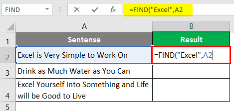
We are going to ignore the start_num argument as it is an optional argument.
Step 4: Close the parentheses to complete the formula and press Enter Key.
If you can see, this function just returned the position where the word “Excel” is present in the current cell (i.e. cell A2).
Step 5: Drag the formula to see the position where Excel belongs under cell A3 and A4.
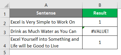
You can see in the screenshot above that the mentioned string is present in two cells (A2 and A3). In cell B3 the word is not present; hence the formula is providing the #VALUE! error. This, however, doesn’t always provide a clearer picture. I mean, someone might not be good enough in excel to understand the fact that 1 appearing in cell B2 is nothing but the position of the word “Excel” in string occupied in cell A2.
Step 6: In order to get a customized result under column B, use the IF function and apply FIND under it. Once you use FIND under IF as a condition, you need to provide two possible outputs. One of the condition is TRUE, the other if the condition is FALSE. Press Enter after editing the formula with IF condition.
After using the above formula, the output is shown below.
Step 7: Drag the formula from cell B2 until cell B4.
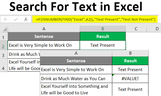
Now, we have used IF and FIND in combinations; the cell with no string still gives #VALUE! error. Let’s try to remove this error with the help of the ISNUMBER function.
ISNUMBER function checks if the output is number or not. If the output is a number, it will give TRUE as a value; if not a number, then it will give FALSE as a value if we use this function in combination with IF and FIND, IF function will give the output based on the values (either TRUE or FALSE) provided by ISNUMBER function.
Step 8: Use ISNUMBER in the formula we used above in step 6 and step 7. Press Enter Key after editing the formula under cell B2.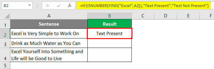
Step 9: Drag the formula across cell B2 to B4.
Clearly the #VALUE! error present in previous steps was nullified due to the ISNUMBER function.
Example #2 – Using SEARCH Function
On similar lines to that of the FIND function, the SEARCH function in excel also allows you to search whether the given substring is present within a text or not. You can use it on the same lines; we have used the FIND function and its combination with IF and ISNUMBER.
SEARCH function also searches the specific string inside the given text and returns the text’s position.
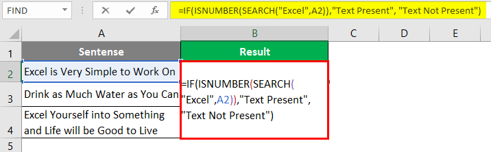
I will directly show you the final formula for finding if a string is present or not in Excel using the combination of SEARCH, IF and ISNUMBER function. You can follow steps 1 to 9, all in the same sequence from the previous example. The only change will be to replace FIND with the SEARCH function.
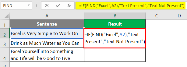
Use the following formula in cell B2 of the sheet “Example 2”, and press Enter Key to see the output (We have the same data as used in the previous example) =IF(ISNUMBER(SEARCH(“Excel”,A1)),”Text Present”, “Text Not Present”) Once you press Enter Key, you’ll see an output the same as in the previous example.
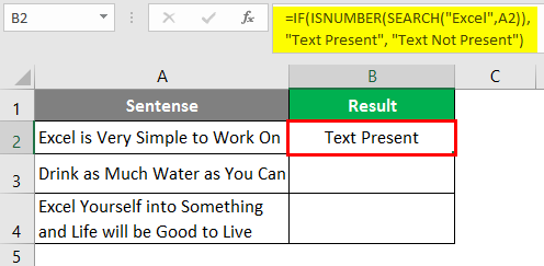
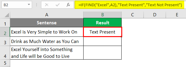
Drag the formula across the cells B2 to B4 to see the final output.
In cell A2 and A4, the word “Excel” is present; hence it has output as “Text Present”. However, in cell A3, the word “Excel” is not present; therefore, it has output as “Text Not Present”.
This is from this article. Let’s wrap the things with some things to be remembered.
Things to Remember About Search For Text in Excel
- These functions are used to check whether the given string is present in the text provided. In case you need to extract the substring from any string, you need to use the LEFT, RIGHT, MID functions altogether.
- ISNUMBER function is used in combination so that you are not getting any #VALUE! error if the string is not present in the text provided.
Recommended Articles
This is a guide to Search For Text in Excel. Here we discuss How to Search Text in Excel along with practical examples and a downloadable excel template. You can also go through our other suggested articles –
- SEARCH Formula in Excel
- Excel Text with Formula
- Formatting Text in Excel
- VBA Text

This program called Excel belongs to the Microsoft company and is currently also known as a spreadsheet . This program allows its users to store in it, text and numerical data and then perform mathematical functions in a much simpler way, as well as perform some statistics functions.
Among other functions, it highlights that it allows you to use different spreadsheets simultaneously, as well as greatly facilitate the work with numbers, either to generate tables and graphs >. In addition, it also gives you the possibility to perform specific searches of either a word or a set of numbers .
That is why here we are going to explain how you can search for a specific word within an Excel file , either through some special functions or with the use of the keys To do this you will need to follow the steps that we will teach you below:
Steps to search and find a word or data within a Microsoft document Excel
It is very possible that when you are creating some document in Excel or once it is finished, you have the need to search for a word or some numerical data in it. > This can become a headache, especially if it is a fairly large document , which can take a long time to perform this type of search .
So, here we are going to explain different methods so you can do this much more quickly and easily. You can achieve this through key combinations or simply by applying some functions within the program. In this way, here are the main methods you should use to search and find a word or data in Excel.
Using the key combination
The first method we present is to search for a word or numerical data through your computer keyboard, a way to find that term either replace it with a new one or simply modify it.
This will require you to follow each of the steps we will teach you below:
- To start with this process the first thing you have to do is enter the Microsoft Excel program, keep in mind that if you don’t have it on the desktop as a icon shortcut you can get it through the start menu.

- Once you enter the program on the left side of your screen you will see the most recent files , in case you want to open another document simply click on “Open other books ” and select the corresponding one.

- Once you are inside the file you want to work on, you can start with this word search process.
- To make sure the window is active You need to click on any of the cells in the spreadsheet.
- Now, you must open the “Search / Replace” window for this you will use the following letter combination with the help of your keyboard ” Ctrl + B ”.

- Once pressed both keys you will see a new window on the computer screen.
- In this new window you must write the word or numerical data you want to find inside the document. Note that you can also enter a phrase exactly the same as it is written in the file, and then click on “Search next” located at the bottom of the window .

- After this Excel will automatically start searching for the matches of the word or number that you have entered in the bar search, > These terms will be highlighted to facilitate your search.
- In case you want to replace the word , number or sentence you just have to click on the tab of “Replace” within the “Search / Replace” window. There will appear two lines, in the first you put the word to search and the second the word by the which one you are going to replace.

Using the «SEARCH»
The SEARCH function is basically to perform search functions when you need to search for information in a specific column or row of the document and thus be able to find a value from it position, but in a different row or column . This method is used especially when you want to have a reference of some specific data, it can be the price of a certain product.
To make this much easier, here is an example:
“If you have a number of inhabitants and want to know the sex of them , you can use this SEARCH function, since when entering the value you want search from cell D8, it will automatically show you the value of cell E8. ”

In order to do this you can do it in two different ways, either in vector or matrix form.
In the case of the vector form , you can use the SEARCH function to find a registered value in either a column or row. This way, you must specify the range that contains the values you want to find . In the case that you want to find a value within column D , you must select the range of it, as well as that of the column where you want to obtain a result.
To be able to do this you will need to enter the formula in the search bar , in the case that we will show you the data of has been used in column D and column F , in this case we wanted to find the value of 3100 to obtain a result of the column F, for this we used the formula = SEARCH ( 3100; D4: D8; F4: F8)

Keep in mind that this formula will vary depending on the columns or rows you want to work with. Once you have established the corresponding formula you just have to press the “Enter” key and immediately you will be thrown a result in the cell you have selected.

Using the function «FIND»
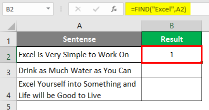
This function aims to be able to search for text strings within another text string, in this way you can return the number of the position of the text string you are looking for in that document Excel.
An example of this FIND function so you can understand this tool a bit more is: “We want to find the location of a letter, in this case it is the“ P ”that corresponds to the word “Printer”, for this we can use this function: = FIND (“P”, “Printer “). Entering this function throws the number 3 , in this case it is 3 because the location of the letter “P” in that word is the third character.
>
Other alternatives that we find with this function is that you can search by word within another word, in this case if we use the word “Average” we can use the function = FIND (“average”; “average”).
In this case, the number 4 is thrown, since the word “medium” begins in the fourth character of the term of “average”. strong> In order to do this keep in mind that you can use both the HALLARB Y HALLAR function, a tool that will allow you to find the location of a character or a text string within another text string.
With the function «FIND»
This function aims to allow us to find a text or just a letter within another text string, in the case of finding a match with the reference we are looking for it will return us to the position of the first letter you got.
This function of FIND is written as follows: FIND (searched_text, within_text_, [initial_number]), inside the searched text you simply enter the letter or word that you want to find, in the space “inside the text” you place the text where you will perform the search and in the “initial_number” the position where the search will begin, the latter is optional, since if is not used the search will start from the first character automatically .
To be able to do this you just have to follow these steps that we will show you below:
- As you can see in this image, the FIND function has been used to find the position of the letter “e” within a text string that is in the “Cell A1”.

- Keep in mind that if you write the letter incorrectly, an error will be thrown at you, as would happen if we put the letter “E” in uppercase, since this character is not found in this text string.

- Now, we can see how this function returns to the position of the first letter “a” for each of the text strings.

- If we want to FIND the second occurrence of the letter “a” in the strings of the text you can use the following formula : = FIND (“a”, A2, FIND (“A”, A2) +1).
- Once this formula has been introduced, you will receive the following result:
