Can you query data in excel - Word и Excel - помощь в работе с программами

Excel for Microsoft 365 Excel 2021 Excel 2019 Excel 2016 Excel 2013 Excel 2010 More…Less

With Power Query (known as Get & Transform in Excel), you can import or connect to external data, and then shape that data, for example remove a column, change a data type, or merge tables, in ways that meet your needs. Then, you can load your query into Excel to create charts and reports. Periodically, you can refresh the data to make it up to date. Power Query is available on three Excel applications, Excel for Windows, Excel for Mac and Excel for the Web. For a summary of all Power Query help topics, see Power Query for Excel Help.

Note: Power Query in Excel for Windows uses the .NET framework, but it requires version 4.7.2 or later. You can download the latest .NET Framework from here. Select the recommended version and then download the runtime.

There are four phases to using Power Query.

Connect Make connections to data in the cloud, on a service, or locally
Transform Shape data to meet your needs, while the original source remains unchanged
Combine Integrate data from multiple sources to get a unique view into the data
Load Complete your query and load it into a worksheet or Data Model and periodically refresh it.

The following sections explore each phase in more detail.

You can use Power Query to import to a single data source, such as an Excel workbook, or to multiple databases, feeds, or services scattered across the cloud. Data sources include data from the Web, files, databases, Azure, or even Excel tables in the current workbook. With Power Query, you can then bring all those data sources together using your own unique transformations and combinations to uncover insights you otherwise wouldn’t have seen.

Once imported, you can refresh the data to bring in additions, changes, and deletes from the external data source. For more information, see Refresh an external data connection in Excel.

Transforming data means modifying it in some way to meet your data analysis requirements. For example, you can remove a column, change a data type, or filter rows. Each of these operations is a data transformation. This process of applying transformations (and combining) to one or more sets of data is also called shaping data.

Think of it this way. A vase starts as a lump of clay that one shapes into something practical and beautiful. Data is the same. It needs shaping into a table that is suitable for your needs and that enables attractive reports and dashboards.

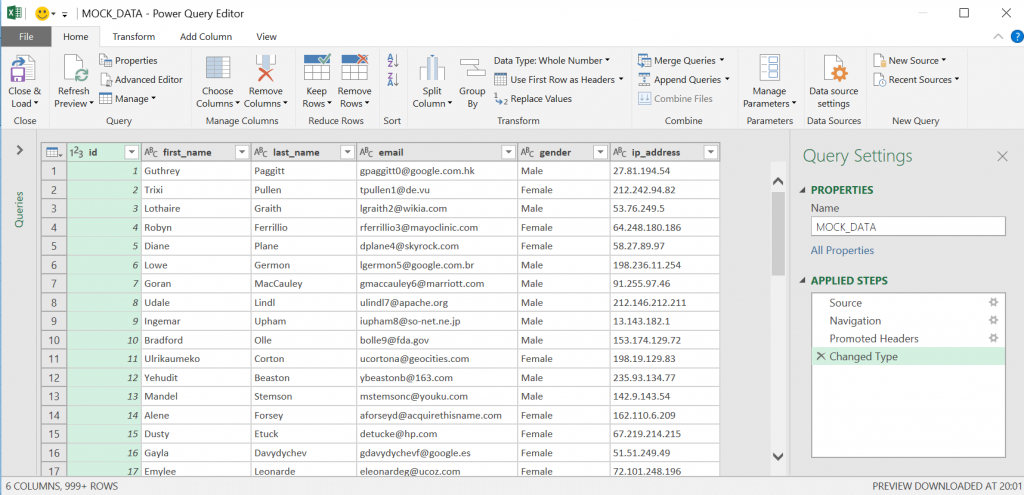
Power Query uses a dedicated window called the Power Query Editor to facilitate and display data transformations. You can open the Power Query Editor by selecting Launch Query Editor from the Get Data command in the Get & Transform Data group, but it also opens when you connect to a data source, create a new query, or load a query.

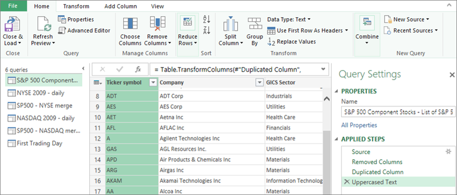
The Power Query Editor keeps track of everything you do with the data by recording and labelling each transformation, or step, that you apply to the data. Whether the transformation is a data connection, a column removal, a merge, or a data type change, you can view and modify each transformation in the APPLIED STEPS section of the Query Settings pane.

There are many transformations you can make from the user interface. Each transformation is recorded as a step in the background. You can even modify and write your own steps using the Power Query M Language in the Advanced Editor.

All the transformations you apply to your data connections collectively constitute a query, which is a new representation of the original (and unchanged) data source. When you refresh a query, each step runs automatically. Queries replace the need to manually connect and shape data in Excel.

You can combine multiple queries in your Excel workbook by appending or merging them. The Append and Merge operations are performed on any query with a tabular shape and are independent of the data sources that the data comes from.

Append An append operation creates a new query that contains all rows from a first query followed by all rows from a second query. You can perform two types of append operations:

Intermediate Append Creates a new query for each append operation.
Inline Append Appends data to your existing query until you reach a final result.

Merge A merge operation creates a new query from two existing queries. This one query contains all columns from a primary table, with one column serving as a navigation link to a related table. The related table contains all rows that match each row from a common column value in the primary table. Furthermore, you can expand or add columns from a related table into a primary table.

There are two main ways to load queries into your workbook:

From the Power Query Editor, you can use the Close and Load commands in the Close group on the Home tab.
From the Excel Workbook Queries pane (Select Queries & Connections), you can right-click a query and select Load To.

You can also fine-tune your load options by using the Query Options dialog box (Select File > Options and settings > Query Options) to select how you want to view your data and where you want to load the data, either in a worksheet or a Data Model (which is a relational data source of multiple tables that reside in a workbook).

For over ten years, Power Query has been supported on Excel for Windows. Now, Excel is broadening Power Query support on Excel for Mac and adding support to Excel for the Web. This means we are making Power Query available on three major platforms and demonstrates the popularity and functionality of Power Query among Excel customers. Watch for future announcements on the Microsoft 365 roadmap and What’s new in Excel for Microsoft 365.

The integration of Get & Transform Data (now called Power Query), into Excel has gone through a number of changes over the years.

Excel 2010 and 2013 for Windows

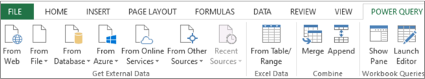
In Excel 2010 for Windows, we first introduced Power Query and it was available as a free add-in that could be downloaded from here: Download the Power Query add-in. Once enabled, Power Query functionality was available from the Power Query tab on the ribbon.

Microsoft 365

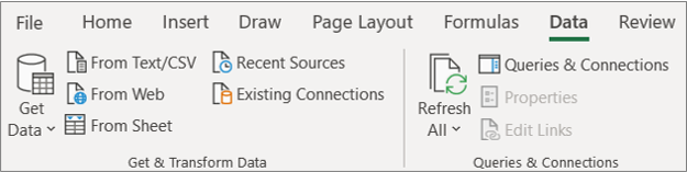
We updated Power Query to be the primary experience in Excel for importing and cleaning data. You can access the Power Query data import wizards and tools from the Get & Transform Data group on the Data tab of the Excel ribbon.

This experience included enhanced data import functionality, rearranged commands on the Data tab, a new Queries & Connection side pane, and the continuing ability to shape data in powerful ways by sorting, changing data types, splitting columns, aggregating the data, and so on.

This new experience also replaced the older, legacy data import wizards under the Data command in the Get External Data group. However, they can still be accessed from the Excel Options dialog box (Select File > Options > Data > Show legacy data import wizards).

Excel 2016 and 2019 for Windows

We added the same Get & Transform Data experience based on the Power Query technology as that of Microsoft 365.

Excel for Microsoft 365 for Mac

In 2019 we started the journey to support Power Query in Excel for Mac. Since then, we added the ability to refresh Power Query queries from TXT, CSV, XLSX, JSON and XML files. We have also added the ability to refresh data from SQL server and from tables & ranges in the current workbook.

In October of 2019, we added the ability to refresh existing Power Query queries and to use VBA to create and edit new queries.

In January of 2021, we added support for the refresh of Power Query queries from OData and SharePoint sources.

For more information, see Use Power Query in Excel for Mac.

Note There is no support for Power Query on Excel 2016 and Excel 2019 for Mac.

Data Catalog deprecation

With the Data Catalog, you could view your shared queries, and then select them to load, edit, or otherwise use in the current workbook. This feature was gradually deprecated:

On August 1st, 2018, we stopped onboarding new customers to the Data Catalog.
On December 3rd, 2018, users couldn’t share new or updated queries in the Data Catalog.
On March 4th, 2019, the Data Catalog stopped working. After this date, we recommended downloading your shared queries so you could continue using them outside the Data Catalog, by using the Open option from the My Data Catalog Queries task pane.

Power Query add-in deprecation

Early in the summer of 2019, we officially deprecated the Power Query add-in which is required for Excel 2010 and 2013 for Windows. As a courtesy, you may still use the add-in, but this may change at a later date.

Facebook data connector retired

Import and refresh of data from Facebook in Excel stopped working in April, 2020. Any Facebook connections created before that date no longer work. We recommend revising or removing any existing Power Query queries that use the Facebook connector as soon as possible to avoid unexpected results.

Excel for Windows critical updates

From June 2023, Power Query in Excel for Windows requires the following components:

Power Query in Excel for Windows uses the .NET framework, but it requires version 4.7.2 or later. For more information, see Update the .NET Framework.
Power Query in Excel for Windows requires WebView2 Runtime to continue supporting the data Web connector (Get Data from Web).  For more information, see Download the WebView2 Runtime.

Need more help?

Источник

26 Sep ’22 by Antonio Nakić-Alfirević

SQL Query function in Excel

If you’re reading this article you probably know that Google Sheets has a QUERY function that allows you to run SQL-like queries against data in the sheet. This function lets you do all sorts of gymnastics with the data in your sheet, be it filtering, aggregating, or pivoting data.

Being a fully-fledged desktop app, Excel tends to be more feature-rich than Google Sheets. This is especially true in the data analytics department where Excel shines with advanced Excel functions as well as Power Query functionality.

However, Excel doesn’t natively have a QUERY function that you can use in cells on the sheet.

In this blog post, I’m going to show you how to add a QUERY function to Excel and give a few examples of how to use it.

First look

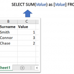
Let’s start by taking a look at the function in action.

Simple SELECT query examples

The function is pretty straightforward. It accepts the SQL query as the first parameter and returns a table with the results of the query.

The results automatically spill to the necessary amount of space. This spilling behavior relies on the dynamic array functionality that’s available in Excel 365 (but isn’t in earlier versions of Microsoft Excel).

Works with Excel tables

In Google Sheets, the QUERY function references data by address (e.g. “A1:B10”) while columns are referenced by letters (e.g. A, B, C…).

This works but has some drawbacks:

It makes the query sensitive to the location of the data. If the data is moved or if columns are reordered, the query will break.
It makes the query difficult to read since it uses range addresses and column letters instead of table and column names (e.g. Employees, DateOfBirth…)
Adding or removing rows can break the query. For example, if the provided range is “A1:H10” the query will only take into account the first 10 rows. If additional rows are added, the query will not take them into account. You can get around this by omitting the end row number (e.g. “A1:H”), but this means that there must be no other content below the data range.

Excel, on the other hand, allows explicitly defining tables (aka ListObjects) that delineate the areas that hold data. Each Excel table has a name, as do its columns. This makes Excel tables very similar to database tables and makes them easier to work with from SQL.

Explicitly defined tables in Excel

Full SQL syntax support (SQLite)

Under the hood, the Windy.Query function is powered by SQLite – a small but powerful embedded database engine.

When called, the function passes the query to the built-in SQLite engine which has an adapter that lets it use Excel tables as its data source.

This means that the entire SQLite syntax is available for use in queries. In comparison, in Google Sheets, the query syntax is rather limited. It only supports a single table (no joins) and a very small set of built-in functions.

Examples of use

Since the engine under the hood is SQLite, queries can use all operations available in SQLite, including table joins, temp tables, column table expressions, window functions etc… Let’s go over some examples of how to use these in Excel.

Joining tables

Here’s an example of a simple one-to-many join:

Simple one-to-many SQL join

The usual way of doing a simple operation such as this one in Excel would be to use xlookup or PowerQuery, but SQL is now another option. And if we needed anything more complex than a simple join, SQL would quickly shine as the most powerful and convenient option of the three.

Merging table rows (union)

Another way we might want to combine two (or more) tables is to combine their rows. We can do this with a SQL UNION operator.

The tables might have some rows in common. If we want to keep only one instance of such rows we would use the regular UNION operator. If we want to keep both versions of rows that are in common, we would use the UNION ALL operator.

Merging rows from two tables

Finding differences between two tables

In the previous example, we had two tables that had some rows in common and some rows not. Let’s assume, for example, that the first table contains last year’s list of employees and the second table is the new list of employees.

If we wanted to find out the differences between the two tables, we could easily do that with a bit of SQL.

All of the rows that are in the first table but not in the second one we will mark as “deleted”. All of the rows that are in the second table but not in the first one we will mark as “added”. Here’s what that SQL query looks like:

select
	id, name, 'deleted'
from
	employees e where not exists (select * from Employees_New en where e.id == en.Id)
union
select
	id, name, 'added'
from
	employees_new en where not exists (select * from Employees e where e.id == en.Id)

And here’s what the result looks like:

Calculating a diff between two tables

Ranking rows

Another useful thing we might want to do is rank rows based on some criteria. For example, suppose we have a table with a list of cities. For each city we have its population and the country it belongs to.

Our task is to find the top 3 cities in each country based on population. Here’s how we might do that in SQL.

-- we use this CTE so we can reference the calculated 'rank_pop' column in the where clause
with cte as (
	select
		city,
		country,
		population,
		-- using the RANK() window function
		RANK() OVER (PARTITION BY country ORDER BY population) as rank_pop
	from
		cities c)
select
	*
from
	cte
where
	-- filtering by the 'rank_pop' column from the CTE
	rank_pop <= 3
order by country, rank_pop

Rank cities by population in each country, return top 3 for each country

This query is a bit more complex than the previous ones. It uses a common table expression and a window function (the rank function), and showcases the ability to write complex SQL in queries.

Queries can also make use of dozens of built-in SQLite functions. Various specialized extended functions such as RegexReplace, GPSDist (GPS distance between two points) and LevDist (fuzzy text matching) are also available.

Updating tables

OK, this next example is a bit of a hack, but a useful one… The query you supply doesn’t need to be a SELECT query. You can do UPDATE/INSERT/DELETE statements as well, and these will modify the data in the target Excel tables.

Updating workbook tables with SQL

This can be a handy way to clean and transform data in your tables in place, without having to export/import the data to an external database (e.g. SQL Server, MySql, Postgres…).

This works because the SQLite engine isn’t copying the data. Rather, it’s using an adapter that lets it access live data in the Excel table.

How does the function see Excel tables?

At first glance, it might seem strange that the query can access your workbook tables. After all, we did not pass them in as parameters, and functions normally only work with parameters that are passed to them.

However, the Windy.Query function is aware of the workbook it’s being called from and it can read data from the workbook’s tables without the need for passing them in as parameters. This makes the function much easier to call especially when working with multiple tables.

Column Headers

Results returned by the Windy.Query function can optionally include headers. This is controlled by the second parameter of the function.

Toggling column headers on/off

The texts in the column headers are determined by the SQL query itself. You can easily rename result columns by aliasing them in the select list.

Aliasing column headers

Automatically refresh results

By default, the SQL query runs as a one-off operation when you enter the formula but does not refresh if the source tables change. However, if you want the query to refresh whenever one of the source tables changes, you can easily do so by setting the autoRefresh argument to true.

Automatic refresh of results when source data changes

Note that the auto-refresh functionality relies on Excel’s RTD (Real-Time Data) server. The RTD server usually throttles updates so functions don’t overwhelm Excel with frequent updates. The default throttle interval is 2s meaning that the function will not update more than once every 2s. To improve responsiveness, you can lower this value to something like 20ms. The simplest way to do this is through the “Configure” dialog in the QueryStorm runtime’s ribbon.

Adjusting the RTD interval in Excel

Passing parameters

When needed, SQL queries can use values from cells as parameters. To use a cell as a parameter in a query, start by giving the cell a name (named range).

Give the parameter cell a name

Once the cell has a name, you can reference it in the query using the @paramName or $paramName syntax.

Use the parameter in the SQL query

If automatic refresh is turned on, results will automatically refresh whenever one of the parameter cells changes its value.

Automatic refresh of results when parameter cell changes

Performance

This is all well and good for small tables, you might think, but how does it handle large data sets? Well, it handles them quite well. The function can read source tables of 100k rows and 10 columns within a few milliseconds and can return this amount of data in a second or two. In addition to this, all columns are automatically indexed so searches and joins are extremely performant as well.

This makes the function perform very well, both from the data throughput standpoint as well as from the computational one.

OK, so is this better than the Google Sheets version of the QUERY function?

Yes, dah. Did you read the previous chapters? 😛

Installing the Windy.Query function

So how do you install this function into your Excel? It’s a simple 2-step process.

Step 1 is to install the QueryStorm Runtime add-in (if you don’t already have it). This is a free, 4MB add-in for Excel that lets you install and use various extensions for Excel. It’s basically an app store for Excel.

Step 2 is to click the “Extensions” button in the “QueryStorm” tab in the Excel ribbon, find the Windy.Query package in the “Online” tab, and install it.

What happens if I share the workbook with a user who doesn’t have the function?

Nothing bad. If the other user doesn’t have the function installed, they will see the last results of the query that were returned on your machine. They just won’t be able to refresh the results.

Advanced SQL query editor

Writing SQL queries in the formula bar can get a bit unwieldy. To make queries easier to write, it’s better to use a proper editor, preferably one that offers syntax highlighting and code completion for SQL and knows about the tables in your workbook.

For this purpose, I recommend using the QueryStorm IDE. This is an advanced IDE that lets you use SQL in Excel. You can write the query in the QueryStorm code editor and then paste the query into the Windy.Query function when you’re happy with it (if needed).

Using the QueryStorm IDE to write SQL queries in Excel

The IDE does more than just allow using SQL in Excel. You can use it to create and share functions and addins for Excel. In fact the QueryStorm IDE was used to create the Windy.Query function itself.

The IDE has a free community version for individuals and small companies, while users in larger companies can make use of the free trial license. For paid licenses, check out the pricing page.

You can read more in this blog post that’s dedicated to the QueryStorm SQL IDE.

Video demonstration

For a video demonstration of the Windy.Query function, take a look the following video:

Источник

You can use Microsoft Query in Excel to retrieve data from an Excel Workbook as well as External Data Sources using SQL SELECT Statements. Excel Queries created this way can be refreshed and rerun making them a comfortable and efficient tool in Excel.

Microsoft Query allows you use SQL directly in Microsoft Excel, treating Sheets as tables against which you can run Select statements with JOINs, UNIONs and more. Often Microsoft Query statements will be more efficient than Excel formulas or a VBA Macro. A Microsoft Query (aka MS Query, aka Excel Query) is in fact an SQL SELECT Statement. Excel as well as Access use Windows ACE.OLEDB or JET.OLEDB providers to run queries. Its an incredible often untapped tool underestimated by many users!

What can I do with MS Query?

Using MS Query in Excel you can extract data from various sources such as:

Excel Files – you can extract data from External Excel files as well as run a SELECT query on your current Workbook
Access – you can extract data from Access Database files
MS SQL Server – you can extract data from Microsoft SQL Server Tables
CSV and Text – you can upload CSV or tabular Text files

Step by Step – Microsoft Query in Excel

In this step by step tutorial I will show you how to create an Microsoft Query to extract data from either you current Workbook or an external Excel file.

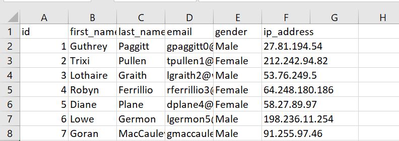
I will extract data from an External Excel file called MOCK DATA.xlsx. In this file I have a list of Male/Female mock-up customers. I will want to create a simple query to calculate how many are Male and how many Female.

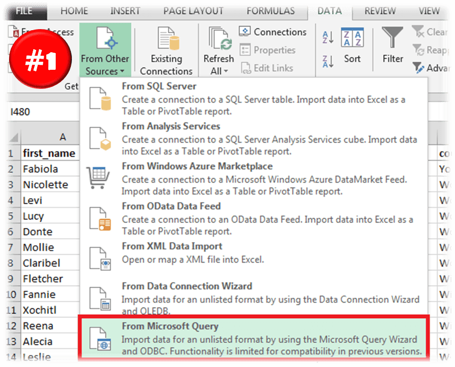
Open the MS Query (from Other Sources) wizard

Go to the DATA Ribbon Tab and click From Other Sources. Select the last option From Microsoft Query.

Select the Data Source

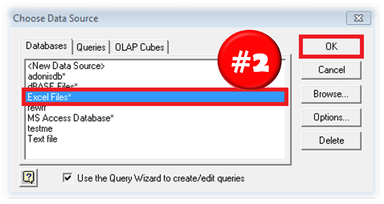Next we need to specify the Data Source for our Microsoft Query. Select Excel Files to proceed.

Select Excel Source File

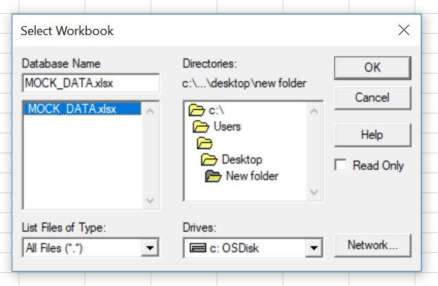Now we need to select the Excel file that will be the source for our Microsoft Query. In my example I will select my current Workbook, the same from which I am creating my MS Query.

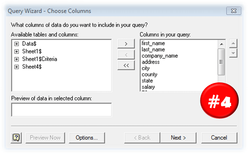
Select Columns for your MS Query

The Wizard now asks you to select Columns for your MS Query. If you plan to modify the MS Query manually later simply click OK. Otherwise select your Columns.

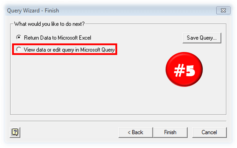
Return Query or Edit Query

Now you have two options:

Return Data to Microsoft Excel – this will return your query results to Excel and complete the Wizard
View data or edit query in Microsoft Query – this will open the Microsoft Query window and allow you to modify you Microsoft Query

Optional: Edit Query

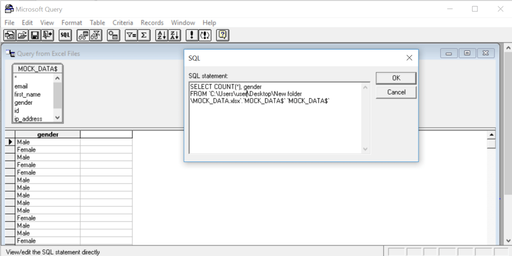If you select the View data or edit query in Microsoft Query option you can now open the SQL Edit Query window by hitting the SQL button. When you are done hit the return button (the one with the open door).

Import Data

When you are done modifying your SQL statement (as I in previous step). Click the Return data button in the Microsoft Query window.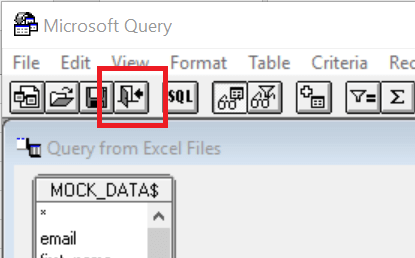
This should open the Import Data window which allows you to select when the data is to be dumped.
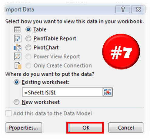Lastly, when you are done click OK on the Import Data window to complete running the query. You should see the result of the query as a new Excel table:

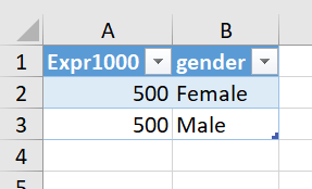
As in the window above I have calculated how many of the records in the original table where Male and how many Female.

AS you can see there are quite a lot of steps needed to achieve something potentially pretty simple. Hence there are a couple of alternatives thanks to the power of VBA Macro….

MS Query – Create with VBA

If you don’t want to use the SQL AddIn another way is to create these queries using a VBA Macro. Below is a quick macro that will allow you write your query in a simple VBA InputBox at the selected range in your worksheet.

Just use my VBA Code Snippet:

Sub ExecuteSQL()
    Attribute ExecuteSQL.VB_ProcData.VB_Invoke_Func = "Sn14"
    'AnalystCave.com
    On Error GoTo ErrorHandl
    Dim SQL As String, sConn As String, qt As QueryTable
    SQL = InputBox("Provide your SQL Query", "Run SQL Query")
    If SQL = vbNullString Then Exit Sub
    sConn = "OLEDB;Provider=Microsoft.ACE.OLEDB.12.0;;Password=;User ID=Admin;Data Source=" &amp; _
        ThisWorkbook.Path &amp; "/" &amp; ThisWorkbook.Name &amp; ";" &amp; _
        "Mode=Share Deny Write;Extended Properties=""Excel 12.0 Xml;HDR=YES"";"
    Set qt = ActiveCell.Worksheet.QueryTables.Add(Connection:=sConn, Destination:=ActiveCell)
    With qt
        .CommandType = xlCmdSql
        .CommandText = SQL
        .Name = Int((1000000000 - 1 + 1) * Rnd + 1)
        .RefreshStyle = xlOverwriteCells
        .Refresh BackgroundQuery:=False
    End With
    Exit Sub
ErrorHandl: MsgBox "Error: " &amp; Err.Description: Err.Clear
End Sub

Just create a New VBA Module and paste the code above. You can run it hitting the CTRL+SHIFT+S Keyboardshortcut or Add the Macro to your Quick Access Toolbar.

Learning SQL with Excel

Creating MS Queries is one thing, but you need to have a pretty good grasp of the SQL language to be able to use it’s true potential. I recommend using a simple Excel database (like Northwind) and practicing various queries with JOINs.

Alternatives in Excel – Power Query

Another way to run queries is to use Microsoft Power Query (also known in Excel 2016 and up as Get and Transform). The AddIn provided by Microsoft does require knowledge of the SQL Language, rather allowing you to click your way through the data you want to tranform.

MS Query vs Power Query Conclusions

MS Query Pros: Power Query is an awesome tool, however, it doesn’t entirely invalidate Microsoft Queries. What is more, sometimes using Microsoft Queries is quicker and more convenient and here is why:

Microsoft Queries are more efficient when you know SQL. While you can click your way through to Transform Data via Power Query someone who knows SQL will likely be much quicker in writing a suitable SELECT query
You can’t re-run Power Queries without the AddIn. While this obviously will be a less valid statement probably in a couple of years (in newer Excel versions), currently if you don’t have the AddIn you won’t be able to edit or re-run Queries created in Power Query

MS Query Cons: Microsoft Query falls short of the Power Query AddIn in some other aspects however:

Power Query has a more convenient user interface. While Power Queries are relatively easy to create, the MS Query Wizard is like a website from the 90’s
Power Query stacks operations on top of each other allowing more convenient changes. While an MS Query works or just doesn’t compile, the Power Query stacks each transform operation providing visibility into your Data Transformation task, and making it easier to add / remove operations

In short I encourage learning Power Query if you don’t feel comfortable around SQL. If you are advanced in SQL I think you will find using good ole Microsoft Queries more convenient. I would compare this to the Age-Old discussion between Command Line devs vs GUI devs…

Источник

We can use queries to extract data from all kinds of data sources. In many cases, it is a more efficient tool than using VBA Macro or formulas. In this tutorial, we will learn how to retrieve data using query from a workbook, Microsoft Access, and many other Microsoft SQL Server tables.

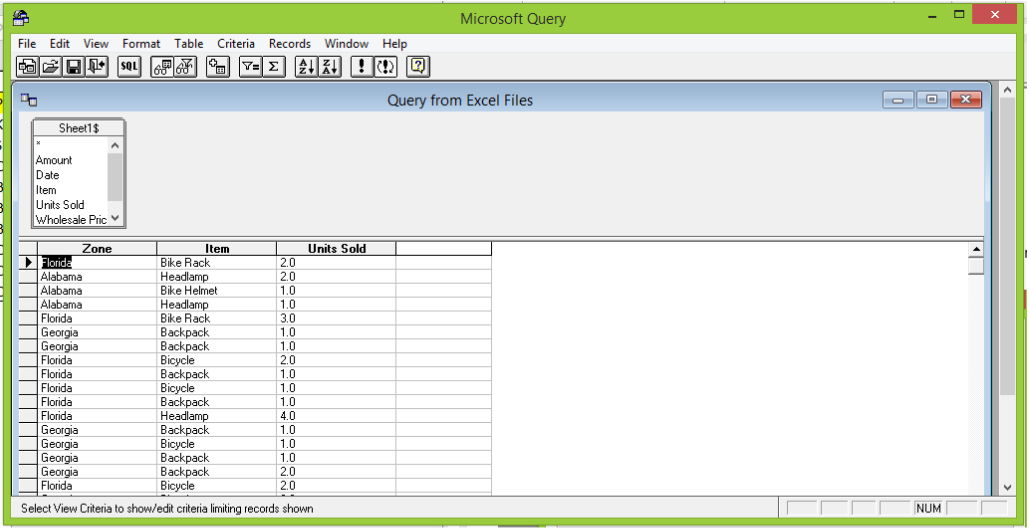Figure 1 – Writing query

Using the Microsoft query tool

In our open Excel document, we will click on Data in the ribbon tab and select From Other sources. If we are using Excel 2016, we will click on Get External Data directly from the Data tab

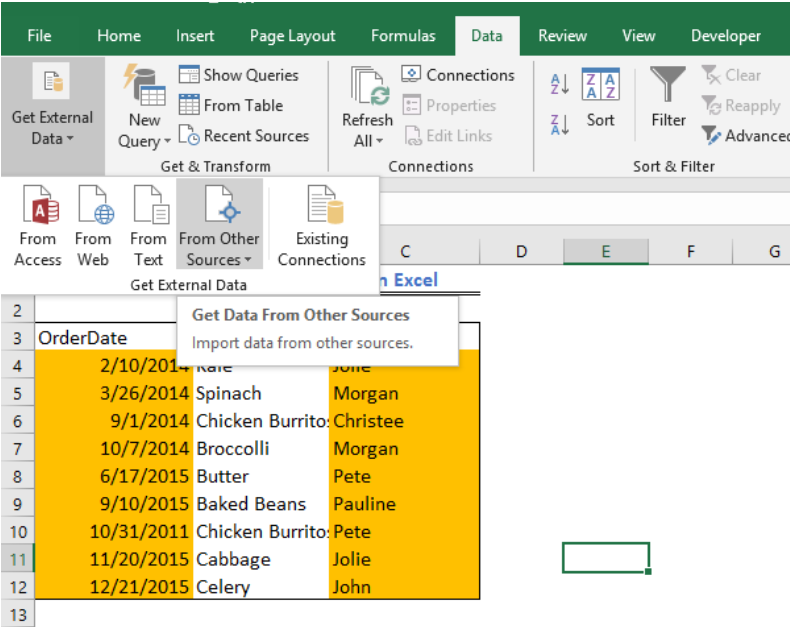Figure 2 – Microsoft query wizard

In the drop-down list, we will select From Microsoft Query

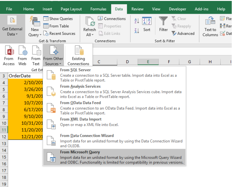Figure 3 – Microsoft query tool

In the Choose Data Source dialog box, we will specify the location of our file. In our example, we want to locate a file, so we will click on files.

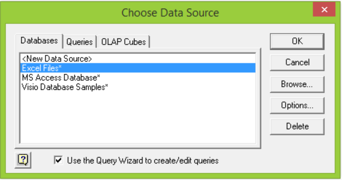Figure 4 – Query access

Next, we will select the file that will be our source for the Microsoft Query.

Figure 5 – Ms query download

We will be asked to pick the columns we want to include in our MS query

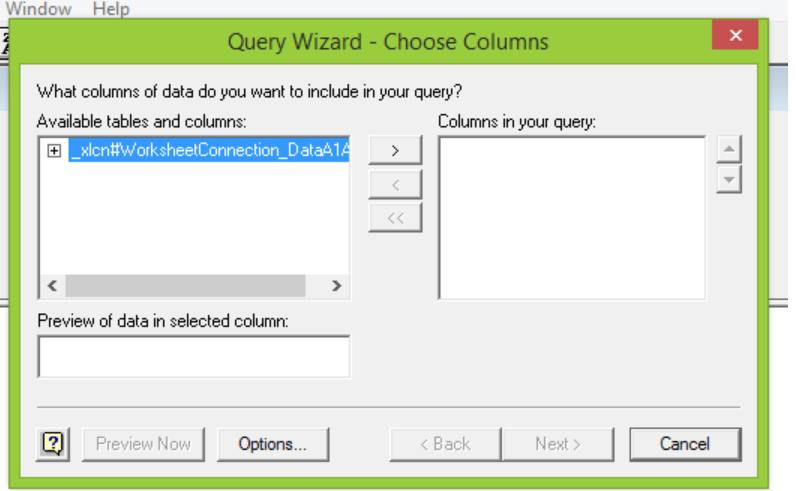Figure 6 – Querying spreadsheet

We will click on the columns we want to include and select Next

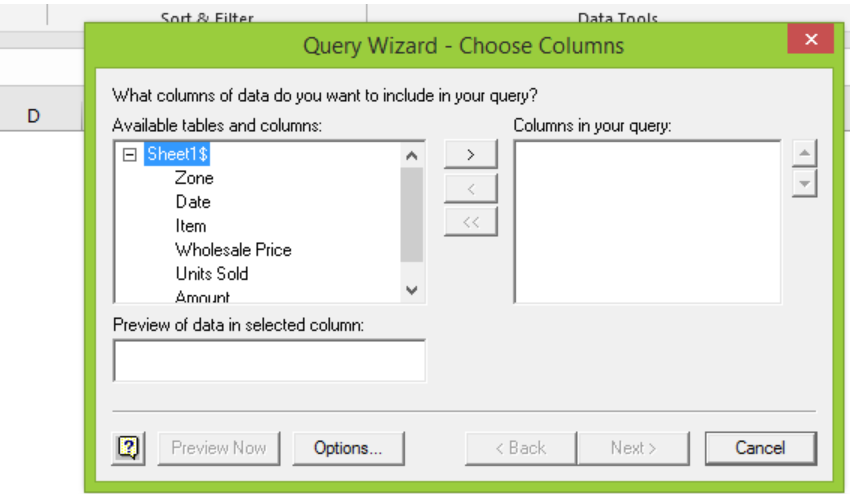Figure 7 – Microsoft query tool

We can filter how we want our data to appear in the next dialog box.

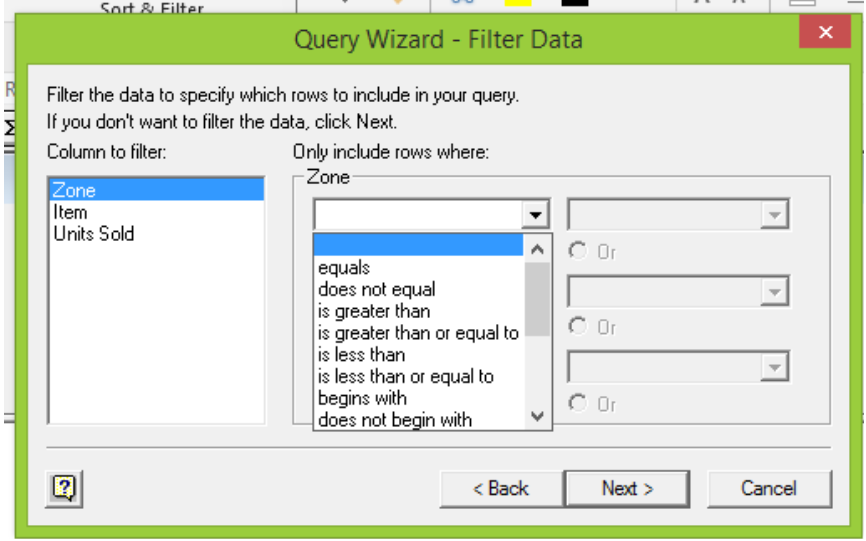Figure 8 – Querying spreadsheet

Next, we will be asked to sort our data. If we don’t want to edit yet, we can click Next

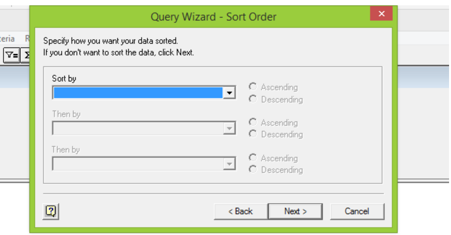Figure 9 – How to use query wizard

The Query Wizard will return with two options. We can either return data to Microsoft Excel or view data or edit query in Microsoft Query

Figure 10 – Excel query

If we selected the View data or edit query in Microsoft Query option, we can open the SQL Edit Query window by clicking on the SQL button

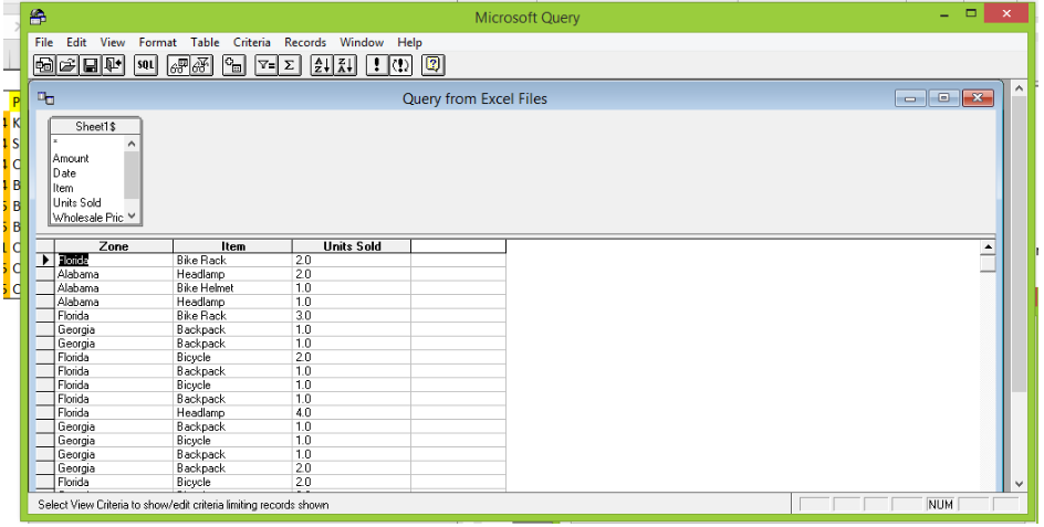Figure 11 – Using the Microsoft Excel Query

When we are done with the edit, we will click on the return button (the open door button as shown below)

Figure 12 – Use the return button to exit the Microsoft Query

After modifying our SQL statement, we will click on return data button in the Microsoft Query window.
Then, in the Import Data dialog box, we can select how we want to view the data and where we want to put the data.

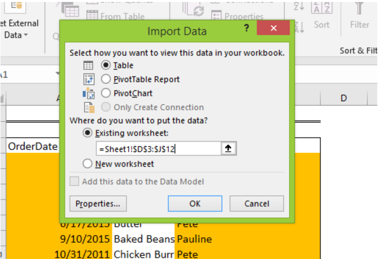Figure 13 – Select how you wish to view your data

Lastly, we will click OK
The result of our query will appear in the new Excel table. Now, we can edit and modify our new table

Figure 14 – Result from using the MS query

Instant Connection to an Excel Expert

Most of the time, the problem you will need to solve will be more complex than a simple application of a formula or function. If you want to save hours of research and frustration, try our live Excelchat service! Our Excel Experts are available 24/7 to answer any Excel question you may have. We guarantee a connection within 30 seconds and a customized solution within 20 minutes.

Источник

Are you dealing with data from a bunch of different places and combine them on a regular basis to do analysis or reporting? Excel Power Query may be the solution you’re looking for! The best thing about this tool is that you can fully automate your data loading and cleaning procedures with a click of a button.

In this tutorial, you’ll learn what Power Query can do and how powerful its features really are. We also provide some practical examples that you can follow to understand basic data transformations using this tool. Let’s get started!

What is Power Query in Excel?

Power Query is a business intelligence tool in Excel used to carry out the ETL (Extract, Transform, and Load) process. This process involves getting data from a source, transforming it, then placing it to a destination for analysis. ETL is known as a crucial step in building a data warehouse, but actually, you’re doing ETL-like processes even if you’re just doing a weekly or monthly report.

What can Power Query do?

With Power Query, everyone can deliver meaningful insight quickly using Excel. There was a time when BI processes required dedicated teams of IT specialists, but not anymore. You can use Power Query as part of your self-service ETL solution to do the following tasks:

#1. Extract (connect and get) data from a source

Power Query allows you to connect instantly with a wide range of data in different formats and locations. Whether your data is in CSV, XML, JSON, or PDF formats, that’s not a problem. Your organization stores data in Azure SQL Database, IBM DB2, Oracle, or PostgreSQL? You can easily access them. Even if you use platforms such as Salesforce and MS Dynamics 365, just connect straight away without hassle!

#2. Transform your data to make it ready for analysis

After connecting to a data source, you may need to modify the data in several ways. Data transformation is the area where Power Query shines. This tool allows for a range of operations, from simple data transformation tasks to the most complex data restructuring challenges, in just a few clicks.

Examples of data transformation tasks:

Data cleaning: Remove duplicates, change data types and formatting, filter rows, split columns, and pivot/unpivot columns.
Data integration: Join or split source tables, add lookup keys, and aggregate data.
Data enrichment: Extend the source data by creating calculated columns.

The ones mentioned above merely scratches the surface of all that Power Query can do to transform your data. The best thing about this tool is that you can automate those data transformation tasks using a code-free interface — without macro or VBA codes.

#3. Load transformed data into a worksheet or the Data Model

After your data is clean and ready for analysis, Power Query Excel gives you options to load your data into one or both of these destinations:

A worksheet. By default, Power Query lands the output data directly in a new worksheet inside your Excel file. If you want, you can place data from each source into a separate worksheet and then do whatever you want with it, just as if it were “normal” Excel data.
The Data Model. Your data is compressed and stored in memory. With this option, you can work with millions, tens of millions, even hundreds of millions of rows of data, exceeding the 1,048,576 row limit of an Excel worksheet!

The Data Model is normally used as the basis for pivot table output in Excel. Thus, it’s also referred to as the Power Pivot Data Model. This article won’t be covering the Data Model and Power Pivot in more detail, as those are broad subjects.

Why use Excel Power Query?

Not only does Power Query allow you to get and transform your data, but this tool also records all the steps applied.

You can refresh all the processes such as re-import the source data, reapply all the data filtering, sorting, and other transformations that you defined — in a single click. So, once all of that’s set up, you don’t need to create it again. Of course, you can also go back and edit each step, and even add steps in between.

This is all done within a tool you’re already familiar with: Excel.

Power Query in different versions of Excel

Power Query for Excel was initially released as an add-in to download and install for Excel 2010 and 2013. After you add Power Query to Excel, a new tab named Power Query will appear in the Excel ribbon.

This tool was fully integrated into Excel by the 2016 version and accessed under the Get & Transform section in the Data tab. So if you use the latest versions of Excel, you already have Power Query integrated within Excel.

The following image summarizes where you can find Power Query in different versions of Excel. Please note that each build of Excel may be slightly different — so you might see slightly different icons.

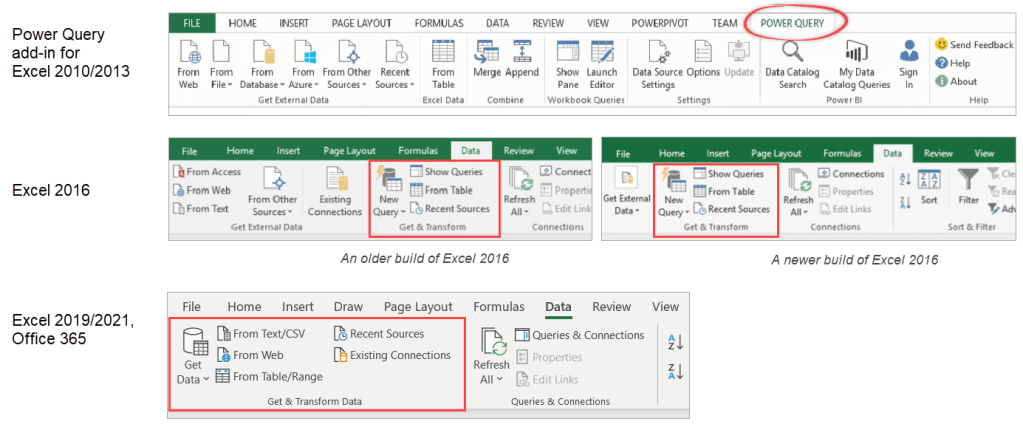
We use Office 365 in this tutorial, however, you can follow the steps described in this article with earlier versions of the product. The entry point into Power Query may be different, but this should not cause any significant difficulties.

Excel Power Query: Download sample files

We provide a small set of sample data used in the examples throughout this article. Just download files from this link to make it easier for you to follow along:

Download sample files

After that, put the CSVs in a folder, for example in “D:/Power Query/Sample files”.

How to use Power Query to GET and LOAD data into Excel

Let’s begin with a quick overview of Power Query’s list of data sources. After that, we’ll get some data into Excel and look into more detail about the Power Query interface.

Power Query list of data sources

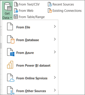
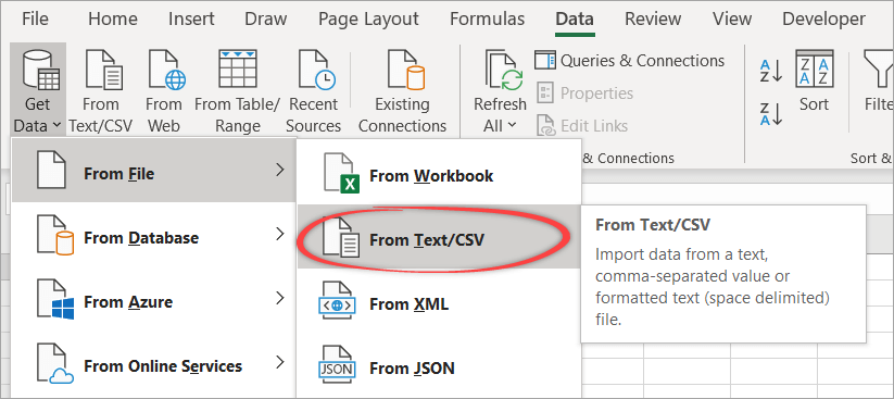
Go to the Data tab and locate Power Query in the Get & Transform Data section. Click on the Get Data button — you will see a dropdown menu to select your data source:

Please note that the range of available Power Query data sources will depend on the version of Excel that you are using.

Data source options

From File: Excel, TXT/CSV, XML, JSON, and PDF.
From Database: SQL Server, Access, Oracle, DB2, MySQL, PostgreSQL, Sybase, Teradata, and SAP Hana.
From Azure: Azure SQL Database, Azure Synapse Analytics, Azure HDInsight (HDFS), Azure Blob, Azure Table, and Azure Data Lake Storage.
From Online Services: Sharepoint Online, Exchange Online, Dynamics 365, Salesforce Objects, and Salesforce Reports.
From Other Sources: Excel Table/Range, Web, OData Feed, ODBC, OLEDB, Active Directory, etc.

If you take a closer look at the Get Data options, you will find that there are currently around 40 data sources for which Power Query connectors are available. However, even this number is small compared to the number of potential data sources out there.

What can you do if your data source is not among those currently available?

One solution is by using a generic data connector such as OData Feed, OLE DB, and ODBC. Another solution is to use an integration tool to help you seamlessly connect and get data from external apps into Excel. An example of this is by using Coupler.io, which is a solution to import data from various apps such as Airtable, Shopify, Jira, QuickBooks, Pipedrive, Hubspot, and more!

Check out the complete list of Coupler.io’s Excel integrations.

A simple example: Get data from CSV files into Excel using Power Query

In the following example, we will import data from two downloaded CSV files one by one and load them into new worksheets.

First, we’ll show you how to get and load Sales.csv directly into a new worksheet. After that, we’ll show you how to import Products.csv and open it in the Power Query Editor before loading it. Here are the steps:

Open a new blank Excel workbook.
Click the Data tab, then click the Get Data button in the Get & Transform Data section.
In the dropdown, select From File > From TXT/CVS.

Browse the folder where you downloaded the sample files. Then, select Sales.csv and click Import.

In the Preview window, click Load to load the data into a new worksheet.

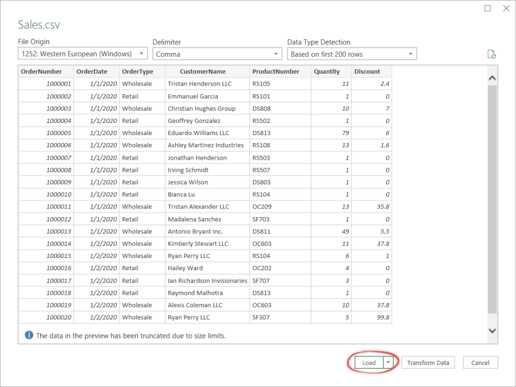
You will see a new worksheet inside the current workbook, as shown in the below screenshot. Your external data is now an Excel table. On the right pane, notice that there is a query to your data source listed there.

Import Products.csv by repeating Steps 1-4 above, but this time, don’t forget to select Products.csv instead of Sales.csv.
In the Preview window, click Transform Data.

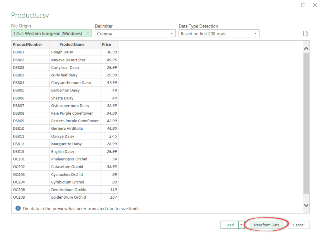
This will open the Power Query Editor as shown in the following screenshot:

As you can see, clicking Transform Data will bring you to a different, separate interface called Power Query Editor. This editor allows you to transform your data before loading it into a new worksheet.

We’ll cover more detail about the Power Query Editor in the next section. For now, let’s not do any data transformations here. We’ll continue to load the products data into a new worksheet from this editor.

Click the small triangle icon in the Close & Load button in the Home tab. Select the first option in the dropdown.

Note: If you choose the second option, you’ll get more options to load your data — more about this in the Load To… options section.

As the final result, you will see a new worksheet created containing the Products table. If you notice, there are two queries listed on the right pane: Sales and Products.

You’ve learned how to get and load two CSV files directly to Excel using Power Query. By the way, you can do something similar using Coupler.io as it includes a CSV to Excel integration as well. You can even set up automatic data refresh on schedule, such as hourly, weekly, and monthly.

Try Coupler.io for free with the seamless Excel integration

Load To… options in Excel Power Query

As explained previously, Power Query provides you with two options to load data: to a worksheet and/or data model. If you want to load data into a worksheet, there are several variations if you choose the Load To… option:

As shown in the above dialog, you can:

Load into an Excel named table (the default)
Load into a pivot table based on the source data
Load into a pivot chart based on the source data
Only create a connection to the data, but do not load it yet

Notice that on top of this, you have the choice of whether you want to create the table of data, pivot table, or pivot chart in an existing or new worksheet.

If you also want to add the data to the Data Model, tick the Add this data to the Data Model checkbox.

Excel Power Query Editor

The Power Query Editor is a separate interface from Excel. All of your data transformations will happen in this editor, which can be launched in one of these two ways:

Click the Get Data button then select Launch Power Query Editor…
Double-click a query listed in the Queries & Connections pane.

Here are the six main elements of Power Query Editor:

The Ribbon. It has 5 main tabs: File, Home, Transform, Add Column, and View.
Query List. This pane contains all the queries that have been added to the current workbook. You can navigate to any query from this area to begin editing it.
Data Preview. This area is where you can see a sample of the data for a selected query.
Formula Bar. This area shows the M code of the current transformation step. Power Query records each of your transformation steps into the M code that you can see in this formula bar. Most of the time, you don’t need to use the M language directly at all.
Properties. This is where you can see and edit the properties of your query. For example, you can rename your query, add a description to it, and enable fast data loading.
Applied Steps. This area contains a list of steps used to transform data.

How to use Power Query to TRANSFORM data in Excel

The range of transformations that Power Query offers are wide and varied. It can be initially daunting if you’re unfamiliar with the feature set available in this tool, but don’t worry! We’ve selected some simple, practical examples for you:

Excel Power Query: Remove duplicates

An external source of data might not be as flawless as you expect. The presence of duplicates is one of the most annoying characteristics of poor quality data.

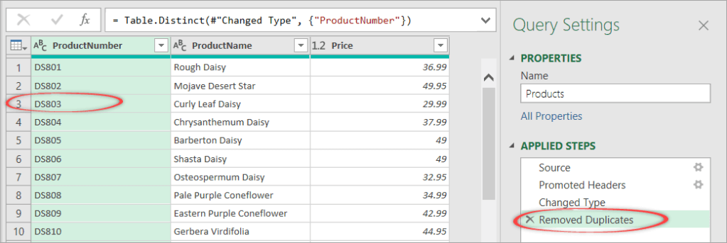
If you look closely at the Products table, you’ll notice two products with ProductNumber DS803.

To remove the above duplicates, follow the steps below:

Launch the Power Query Editor and make sure to select the Products query.

In the Home tab, click Remove Rows > Remove Duplicates.

Notice that one of the rows with ProductNumber DS803 is now removed and a step added in the APPLIED STEPS pane:

Click the Close & Load button. This will refresh the Products table in your worksheet.

Excel Power Query: Create parameters for folder paths

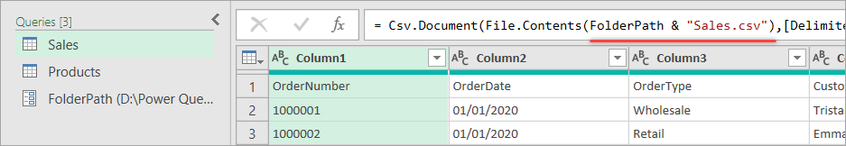
In the Power Query Editor, let’s open the Products query and click on the first row “Source” in the APPLIED STEPS. You will see a hard-coded file path like shown below:

If you check on the Sales query, you’ll notice that it also uses a fixed value for the file path, i.e., D:Power QuerySample filesSales.csv

Changing the folder path to use a parameter can be a time-saver in the future. In case you need to move your files to another folder later, you’ll only need to change the parameter value once.

Let’s do the following steps to replace the hard-coded folder path with a parameter:

In the Home tab, click Manage Parameters > New Parameter.

Create a new parameter using the following details, then click OK.
1. Name: FolderPath
2. Required: ✔
3. Type: Text
4. Suggested Values: Any value
5. Current Value: D:Power QuerySample files

Select the Products query, then click “Source” in the APPLIED STEPS.
In the formula bar, replace the folder path to use the FolderPath parameter:

FolderPath & "Products.csv"

Now, select the Sales query, then click “Source” in the APPLIED STEPS.
In the formula bar, replace the folder path to use the FolderPath parameter:

FolderPath & "Sales.csv"

Now, you’ve changed the file path of both queries to use the FolderPath parameter. Please be aware that the code in the formula bar is case-sensitive. Also, notice that you don’t need to enclose parameters with double quotes.

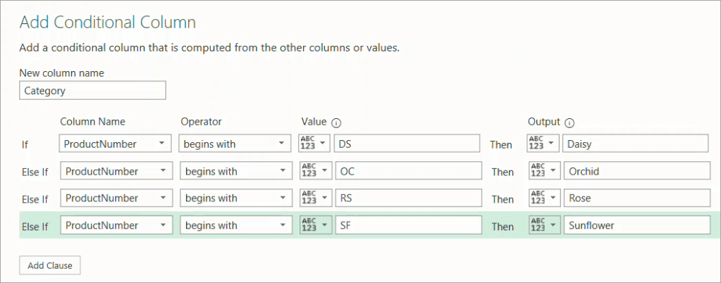
Excel Power Query: Adding a conditional column with IF statement

Suppose you want to create a new column, i.e., Category in the Products query, that tells you which category each product belongs to. The first 2 digits of the product number identify the product category based on the following rules:

Product number begins with “DS” → Daisy
Product number begins with “OC” → Orchid
Product number begins with “RS” → Rose
Product number begins with “SF” → Sunflower

Here’s how you can add the Category column:

Open the Power Query Editor and select the Products query.
Click the Add Column tab, then click Conditional Column.

In the “Add Conditional Column” dialog that appears, enter the following details, then click OK when done.

Click File > Close & Load.
Notice that your worksheet containing the Products table will have the new Category column, as shown below:

Excel Power Query: Drill-down to create parameters from cell

Suppose you want to be able to filter products by category from a cell as shown in the below image:

To pass the value from cell B3 to the query and use it to filter the products, follow the steps below:

Create a new worksheet, e.g. Sheet4, then add the following details:
1. Cell B2: A text “Category”.
2. Cell B3: A dropdown containing a list of product categories: Daisy, Orchid, Rose, and Sunflower. You can create the dropdown using Data > Data Validation with details as follows:

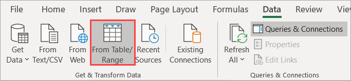
Click Data > From Table/Range.

Figure 29. Creating a query From Table Range

In the “Create Table” dialog, enter the following details, then click OK.
1. Table range: =$B$2:$B$3
2. My table has headers: ✔

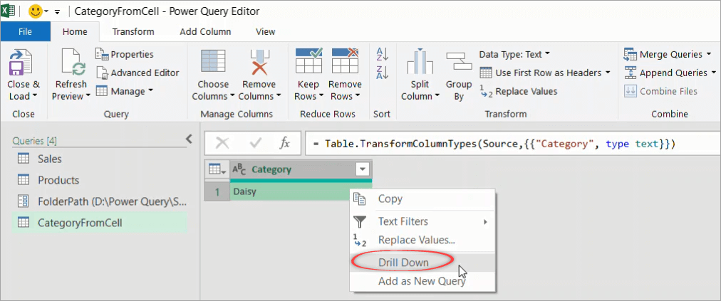
In the Power Query Editor that opens, rename the new query to CategoryFromCell.

Right-click on the data and select Drill Down.

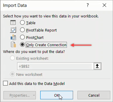
Click File > Close & Load To…
In the “Import Data” dialog, select Only Create Connection.

Figure 33. Choosing to only create a connection

Reopen the Power Query Editor.
Right-click on the Products query and select Duplicate. Rename the new query as ProductsByCategory.

Add a filter by category by selecting the small triangle icon in the Category column, then choose Text Filters > Equals.

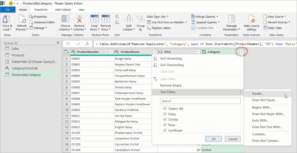
In the Filter Rows dialog, type “Daisy”, then click OK.

In the Formula Bar, change the text “Daisy” to use the CategoryFromCell parameter.

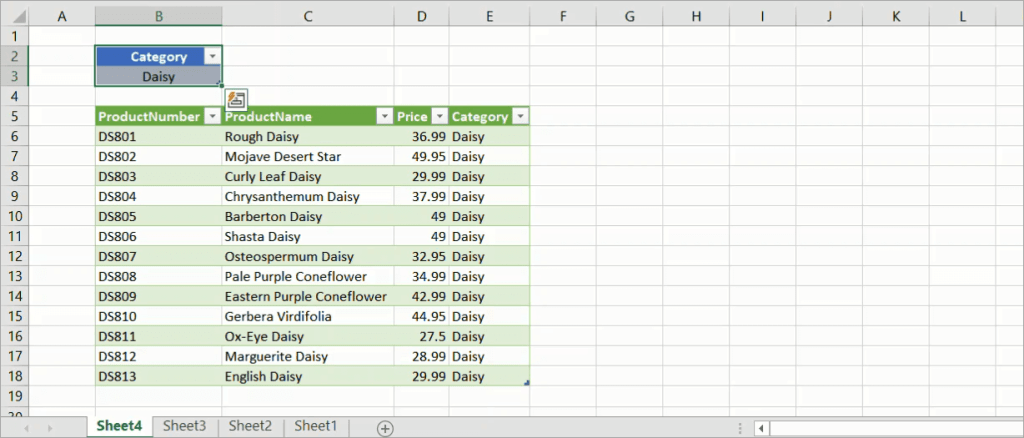
Click File > Close & Load To… Then, in the “Import Data” dialog, select to load to the existing worksheet Sheet4!$B$5 and click OK when done.

Your final worksheet will look like this below. Test by changing the dropdown value to “Rose”, then click the Refresh All button.

Excel Power Query: Merge tables

Merging queries allows you to join tables based on a key column. This is like using VLOOKUP Excel. For example, here we’re going to merge the Sales and Products queries into one. We will retrieve columns from the Products table (the lookup table) and pull them into the Sales table.

Here are the steps:

Launch the Power Query Editor and select the Sales query.
Click Merge Queries in the Home tab, then select Merge Queries as New.

Note: As you can see, you have two options for merging. You can either overwrite the current Sales query with additional columns or merge two queries as a new one to keep your current Sales table unchanged.

In the “Merge” dialog box, select Products as the second table. Then, select the ProductNumber column for both tables and click OK.

If you want, rename the new query as ProductSales_Merge by changing the query name in the Properties pane.
Expand the Products table and select ProductName, Price, and Category columns to include in the query.

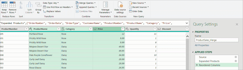
If you want, reorder the columns by moving them to the position you want, the same way you move columns in Excel.

Here’s an example after we moved the ProductNumber, Category, and Price columns before the Quantity and Discount columns.

Click File > Close & Load to load the query into a new worksheet.

Excel Power Query: Using formulas

Suppose that in the ProductSales_Merge query, we want to add a new column OrderTotal which is calculated from other columns using this formula:

OrderTotal = Price * Quantity - Discount

To do that, follow the steps below:

Launch the Power Query Editor and select the ProductSales_Merge query.
In the Add Column tab, click Custom Column.

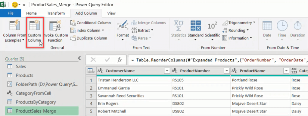
In the “Custom Column” dialog that appears, enter the following details then click OK.
1. New column name: OrderTotal
2. Custom column formula: = [Price] * [Quantity] - [Discount]

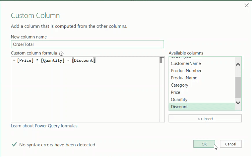
Notice that a new column OrderTotal was added:

Click File > Close & Load.

Excel Power Query: Using functions

In this last example, we’ll show you how to use functions in Power Query. We’ll add a new column Quarter that represents the number of the quarter from the order dates.

Launch the Power Query Editor and select the ProductSales_Merge query.
In the Add Column tab, click Custom Column.
In the “Custom Column” dialog that appears, enter the following details, then click OK.
1. New column name: Quarter
2. Custom column formula:
  = "Q"&Number.ToText(Date.QuarterOfYear([OrderDate]))

Explanation:

The Date.QuarterOfYear() function returns the number of the quarter (1-4) from a date, while the Number.ToText() function converts a number to text format.

Notice that a new column Quarter was added.

Click File > Close & Load to refresh your worksheet.

What’s next?

We’ve covered the basics of how you can use Excel Power Query to get, transform, and load data in Excel. We hope this tutorial has given you a great starting point working with Excel Power Query. Be sure to continue learning about Excel’s Data Model and Power Pivot if you want to master Business Intelligence using Excel.

In addition to importing your data into Excel, take a look at Coupler.io. This excellent integration tool may be a great solution you need if your data source is not among those currently available in Power Query. With this tool, you can import data from different apps into Excel — no coding required. You can also automate the import process on the schedule you want!

Senior analyst programmer

Back to Blog

Focus on your business

goals while we take care of your data!

Try Coupler.io

Источник

Need more help?

26 Sep ’22 by Antonio Nakić-Alfirević

SQL Query function in Excel

First look

Works with Excel tables

Full SQL syntax support (SQLite)

Examples of use

Joining tables

Merging table rows (union)

Finding differences between two tables

Ranking rows

Updating tables

How does the function see Excel tables?

Column Headers

Automatically refresh results

Passing parameters

Performance

OK, so is this better than the Google Sheets version of the QUERY function?

Installing the Windy.Query function

What happens if I share the workbook with a user who doesn’t have the function?

Advanced SQL query editor

Video demonstration

What can I do with MS Query?

Step by Step – Microsoft Query in Excel

Open the MS Query (from Other Sources) wizard

Select the Data Source

Select Excel Source File

Select Columns for your MS Query

Return Query or Edit Query

Optional: Edit Query

Import Data

MS Query – Create with VBA

Learning SQL with Excel

Alternatives in Excel – Power Query

MS Query vs Power Query Conclusions

Using the Microsoft query tool

Instant Connection to an Excel Expert

What is Power Query in Excel?

What can Power Query do?

#1. Extract (connect and get) data from a source

#2. Transform your data to make it ready for analysis

#3. Load transformed data into a worksheet or the Data Model

Why use Excel Power Query?

Power Query in different versions of Excel

Excel Power Query: Download sample files

How to use Power Query to GET and LOAD data into Excel

Power Query list of data sources

Data source options

What can you do if your data source is not among those currently available?

A simple example: Get data from CSV files into Excel using Power Query

Load To… options in Excel Power Query

Excel Power Query Editor

How to use Power Query to TRANSFORM data in Excel

Excel Power Query: Remove duplicates

Excel Power Query: Create parameters for folder paths

Excel Power Query: Adding a conditional column with IF statement

Excel Power Query: Drill-down to create parameters from cell

Excel Power Query: Merge tables

Excel Power Query: Using formulas

Excel Power Query: Using functions

What’s next?

Focus on your business goals while we take care of your data!

Focus on your business

goals while we take care of your data!