
![]()
Download Article
![]()
Download Article
This wikiHow teaches you how to name columns in Microsoft Excel. You can name columns by clicking on them and typing in your label. You can also change the column headings from letters to numbers under settings, but you cannot rename them completely.
-

1
Open Microsoft Excel on your computer. The icon is green with white lines in it. On a PC it will be pinned to your Start Menu. On a Mac, it will be located in your Applications folder.
-
2
Start a new Excel document by clicking “Blank Workbook”. You can also open an existing Excel document if you click Open other Workbooks.
Advertisement
-
3
Double-click on the first box under the column you want to name.
-
4
Type in the name that you want. The headers at the top (letters A-Z) will not change as those are Excel’s way of keeping track of information within your document. However, when you type in a name for column A1 that will become the name for the rest of the “A” column.


Advertisement
-
1
Open Microsoft Excel on your computer. The icon will be green with white lines. On a Windows PC, it will be pinned to your Start Menu. On a macOS, it will be in your Applications folder.
-
2
Start an Excel document by clicking on “Blank Workbook”. You can also open an existing Excel document if you click Open other Workbooks.
-
3
Click on Excel and then Preferences on a Mac.
- On a PC click File and then Options.
-
4
Click on General on a Mac.
- On a PC click Formulas.
-
5
Click the box next to “Use R1C1 Reference Style.» Press Ok if prompted. This will change the header columns from letters to numbers.


Advertisement
Ask a Question
200 characters left
Include your email address to get a message when this question is answered.
Submit
Advertisement
Thanks for submitting a tip for review!
About This Article
Article SummaryX
1. Open your Excel document.
2. Double-click on the first box under the column you want to rename.
3. Type in the name you want and press enter.
Did this summary help you?
Thanks to all authors for creating a page that has been read 44,598 times.
Is this article up to date?
While many people will use a header row in their spreadsheets to identify the information that is contained within a column, that might not be useful for what you need to do.
Another option that you have involves learning how to name a column in Excel.
This gives you some additional flexibility with cell references and formulas, which may be more optimal for the way that you use Excel.
Our tutorial below will show you how to name columns in Excel so that you can start taking advantage of the additional features this enables.
- Open your spreadsheet.
- Click the column letter to rename.
- Click in the Name field next to the formula bar.
- Delete the current name.
- Enter the new name, then press Enter.
Our article continues below with additional information on naming columns in Excel for office 365, including pictures of these steps.
When you need to reference a specific cell in Microsoft Excel it is common for you to use row numbers and column letters. These are shown at the left side and top of the spreadsheet, respectively, and provide an easy way to locate cells for formulas.
But you may be looking for a way to create custom column names in Excel if you don’t want to use the default column headings.
This can be useful when you are working with a lot of similar data and are running into problems with properly identifying columns. It can also be a useful way to may writing formulas easier because you can just enter your custom name into the formula rather than going back to see which column contains which data.
Fortunately, it is possible for you to give a column a name in Excel if you would like to be able to reference the column by that name rather than the standard column letters.
How to Rename a Column in Excel (Guide with Pictures)
the steps in this article were performed in the desktop version of the Microsoft Excel for Office 365 application. However, these steps will also work in most other versions of Excel.
These steps will show you how to label columns in Excel.
Step 1: Open the Excel file containing the column you wish to rename.
Open your spreadsheet.
Step 2: Click the column letter above the spreadsheet.
Choose the letter of the column to name.
Step 3: Click inside the Name field that is above the row numbers and to the left of the formula bar.
Select the Name field.
It is at the upper left corner of the Excel worksheet, above the row numbers and to the left of the column letters.
Step 4: Delete the current column name.
Remove the existing column name.
Step 5: Type the new name, then press Enter on your keyboard.
Input the new column name and press Enter.
Now that you know how to name a column in Excel you can take advantage of this when you are working on spreadsheets that need column names.
The next section discusses editing a column header in Excel.
How to Change a Column Header in the Name Box Dropdown List in Microsoft Excel
The steps above walk you through the process of how you create names for single columns in an Excel spreadsheet. Once you have elected to give a new, custom name rather than the default Excel names for some of your columns, then those custom names are going to appear in a dropdown list within the Name field.
You can quickly select a column and choose to rename one of these column headers by simply clicking inside that Name field and choosing the column name. That will select that column. You can then click inside the Name field again, delete the current name, enter a new name, then press Enter.
Our guide continues below with more information, such as what to do if you are seeing an error when trying to name columns in Excel.
More Information on How to Name Columns in Excel
If the row numbers and columns aren’t visible in Microsoft Excel then they have probably been hidden. You can display them by selecting the View tab at the top of the window, then checking the box next to Headings in the Show group of the ribbon.
If you are having trouble giving your column a name, then it may be because you are attempting to include a space. In my example above I am giving my column the name “LastName” but I would get an error if I tried to give it a name of “Last Name.”
Once a column is renamed you can do stuff like =SUM(LastName) to quickly add all of the values in that column.
One helpful thing that you can do when you have renamed columns in Excel is to quickly select an entire column by its name. if you click the arrow in the Name field you will see a dropdown list with all of your custom column names. If you select one of those names it will automatically highlight that entire column.
These column names are a little different than creating titles in the first row of each column. Traditionally that is used as a simple way to identify what type of data is in a column. It also makes it very easy to use the “Print Titles” button on the Page Layout tab so that you can repeat the top row of your spreadsheet on every page.
it is possible for you to use the first row as a title row in Microsoft Excel while still creating custom column names using the steps outlined in the tutorial above.
One additional similar action you can take is to create an Excel named range that consists of a few cells. You can use your mouse to select the cells to include in that range, then click inside the Name field, delete the current name, enter the new one, then press Enter on the keyboard. When you start creating more and more named ranges in your spreadsheet you can really make selections quickly by clicking the Name Manager to cycle through all of your defined names group values.
Frequently Asked Questions About How to Name a Column in Excel
Are headers and column names the same thing in Excel?
No, these are two different things.
A header in Excel is the first row of the spreadsheet, where you can enter a word or phrase that describes the information that will appear in cells in that column.
A name is something that you apply with the special “Name” field to the left of the column letters.
An Excel header and name can have the same values, but they serve different purposes.
Often row headers will be sufficient for an Excel sheet.
Where is the Excel formula bar?
you can find the formula bar in your Excel spreadsheet above the column letters.
It is possible to hide the formula bar, however, you can also go to the View tab, then make sure that the Formula Bar option in the Show group is checked.
How do I delete a column in Microsoft Excel?
If you have a column in your Excel document that you don’t need anymore, then you are able to remove it.
You can do this by right-clicking on the column letter, then choosing the Delete option.
You can also use this option to delete multiple columns.
Simply hold down the Ctrl key on your keyboard, then click each column letter that you want to remove.
Once all of the columns are selected you can right-click on one of them and choose the Delete option.

Matthew Burleigh has been a freelance writer since the early 2000s. You can find his writing all over the Web, where his content has collectively been read millions of times.
Matthew received his Master’s degree in Computer Science, then spent over a decade as an IT consultant for small businesses before focusing on writing and website creation.
The topics he covers for MasterYourTech.com include iPhones, Microsoft Office, and Google Apps.
You can read his full bio here.
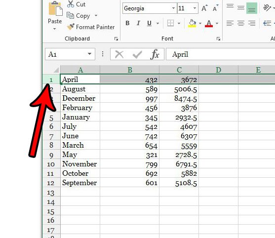
Adding a row of headings to the top of your spreadsheet is an effective way to describe the data in your cells. This is especially important when a printed sheet extends across multiple pages. but you might be asking how do you name columns in Excel if you have already entered all of your data and didn’t leave a blank row at the top.
How to Create Excel Column Names
- Open your spreadsheet.
- Select the top row number.
- Right-click the selected row and choose Insert.
- Enter column names in the blank row.
Our guide continues below with additional information to answer the question of how do you name columns in Excel, including pictures of these steps.
Putting descriptions for columns at the top of your spreadsheet is a great way to label your data and make it easier to understand.
This is such a common practice that Excel actually gives a name to it, which is the “title row.” You can even choose to freeze that title row if you would like it to remain visible when you scroll down your spreadsheet.
Our tutorial below will show you how to insert a new row at the top of your spreadsheet so that you can use it as a title row.
We will also discuss how to turn a selection with title rows into a table in Excel so that you can perform other actions on your data, such as filtering and sorting.
Check out our Microsoft Excel add column tutorial and learn about easy ways to get sums of cell data.
How to Add a Title Row to a Spreadsheet in Excel 2013 (guide with Pictures)
The steps in this article were performed in Microsoft Excel 2013. These steps will work in other versions of Excel as well. We will also discuss turning a selection of cells into a table in Excel in the section below, which may be closer to the result you are trying to achieve, if adding the title row isn’t the desired result.
Step 1: Open your spreadsheet in Excel 2013.
Step 2: Click the top row number at the left side of the spreadsheet.
If you haven’t hidden any rows, then this should be row 1.
Step 3: Right-click the selected row number, then choose the Insert option.
You can also insert a new row when a row is selected by pressing Ctrl + Shift + + on your keyboard.

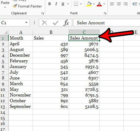
Step 4: Add column names into the blank cells in this new row.
Our article continues below with another answer to the question of “how do you name columns in Excel” which involves creating a table from your existing data.
How to Turn a Selection Into a Table in Excel 2013
Now that you’ve added your column names, you can go one step further by turning a selection into a table with the steps below.
For more information, you can read our complete guide to creating tables in Excel.
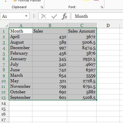
Step 1: Select the cells that you want to include in the table.
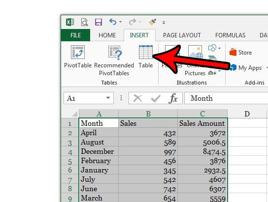
Step 2: Click the Insert tab at the top of the window.

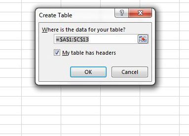
Step 3: Select the Table button in the Tables section of the ribbon.
Step 4: Confirm that the My table has headers option is checked, then click the OK button.
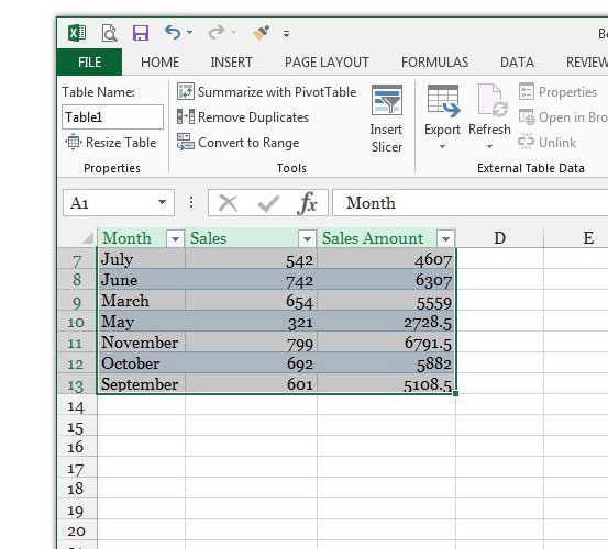
If you scroll down in your table you will see that the table column names replace the column letters while the table is still visible.
Hopefully this has helped you to answer the question of how do you name columns in Excel?
Now that you’ve set up your table in the manner that you want, one of the next hurdles will be getting it to print properly. Check out our Excel printing guide for some tips on making your spreadsheet a little easier to manage when it’s printed on paper.
Additional Sources

Matthew Burleigh has been writing tech tutorials since 2008. His writing has appeared on dozens of different websites and been read over 50 million times.
After receiving his Bachelor’s and Master’s degrees in Computer Science he spent several years working in IT management for small businesses. However, he now works full time writing content online and creating websites.
His main writing topics include iPhones, Microsoft Office, Google Apps, Android, and Photoshop, but he has also written about many other tech topics as well.
Read his full bio here.
The default method for including a column reference in an Excel formula is to use the column letter, a convention that may make it difficult to interpret the parts of complex formulas. Microsoft designed Excel with a method for naming cell ranges and columns to simplify writing and interpreting formulas. You can apply column names to a single worksheet or increase the scope and apply it to an entire workbook.
Single Sheet
-
Click the letter of the column you want to rename to highlight the entire column.
-
Click the «Name» box, located to the left of the formula bar, and press «Delete» to remove the current name.
-
Enter a new name for the column and press «Enter.»
Workbook
-
Click the letter of the column you want to change and then click the «Formulas» tab.
-
Click «Define Name» in the Defined Names group in the Ribbon to open the New Name window.
-
Enter the new name of the column in the Name text box.
-
Click the «Scope» drop-down menu and select «Workbook» to apply the change to all of the sheets in the workbook. Click «OK» to save your changes.
How to Name a Range in Excel: Step-by-Step (+ Name Manager)
Excel is all about storing data and doing something with it. And to make data storage and manipulation easier, Excel allows users to name their data.
You can name different ranges (or arrays) in Excel and the Excel Name Manager will store them for you. Once saved, you can refer to that range of cells simply by using its name.
So instead of referencing a range like this =SUM($A$2:$C$250), write the name you gave it, which could be something like this =SUM(Prices).
Looks much easier, right? 💡
Practicing something in real-time can make you 10x faster at it. And you can master naming ranges in Excel with our sample workbook for free. Grab it here.
How to name a range in excel
A named range can save you a lot of time and confusion. And if you haven’t used it before, take my word for it – it’s very easy to create a named range.
It literally takes less than five seconds – unless, of course, the name you assign is extremely long 😅
Let’s see a simple example of naming a range below.
We have the following data.

I want to name the range A2:A10 as ‘Tableof5’.
For that:
- Select the range.

- Click in the Name Box

- Assign a name to the cell range.
- Press Ok.

The selected range has now been named.
Excel will show you the name of the range when you select it.
Important note:
Note that the name of a range cannot contain space. If you add space in the Name Box, Excel will show an error prompt:

Similarly, the first character of the name cannot be a digit. And names cannot have any other symbol other than period, backslash, and underscore character. Also, the name must not exceed 255 characters.
How to use a named range in a formula
Named ranges make writing formulas easier and quicker. Usually, you would type a formula, select all the cell references and then press Enter.
But with named ranges, you just need to enter the name of the range in place of the arguments. And it’s done 🤓
Let’s see how to use a named range in the formula below.
We will use our previous data set for this example.
We want to calculate the AVERAGE of the values of the sample data. For that:
- Name the range you want to use in the formula.
- In a cell, type in the formula.

- Enter the named range in place of the argument.

As evident, the formula immediately picks up the named range.
Note that Excel only shows the name of the range when you select the entire range. If you simply select a single cell from that range, it will show the selected cell’s reference. And not the name of the range.
- Press Enter.

Excel returns the AVERAGE of the named range.
Pretty easy, no? 😃
How to use the name manager in excel
Using names for ranges can be really useful – especially when working with an exceptionally large worksheet.
But it can be equally confusing too.
You can’t possibly readily remember the names of 32 ranges and their exact location. And figuring it out manually will leave you with no time.
Luckily, we have the Name Manager in Excel for this purpose.
As evident from the name, the Excel Name Manager is like the index page where all named ranges and cells are stored. You can also find the location of all named ranges in your Excel worksheet.
Let’s understand the Name Manager’s work in more detail below.
To open it:
- Go to the Formulas Tab.
- Select Name Manager from the Defined Names group.

- The Name Manager dialog box appears.

The Name Manager shows our previously created named range. It also shows which cells the named range refers to.
PRO TIP!
You can open the Excel Name Manager in seconds using the shortcut ALT + M + N. Cool, no? 😎
You can find all your named ranges in one place, thanks to the Name Manager. This makes it extremely useful, especially if you have plenty of named ranges.
There’s also a Filter button at the top right corner of the dialog box. It offers a menu of options that you can choose to perform different operations.
Edit named ranges
Just like adding and deleting named ranges, you can edit them too. You can access the Edit feature from the Name Manager dialog box.

You can edit the name of the range, change its reference, and even add comments.
Say, we want to change our named range ‘Tableof5’ to ‘Multiplesof5’.
For that:
- Click Edit from the Name Manager dialog box.
- The Edit Name dialog box appears.

- Click in the Name box and enter the desired name.
- Press Ok.

You can also change the references if you want to add or delete a field from the ‘Refers to’ box. It is at the bottom of the Edit Name dialog box.
Or you could do it directly from the Name Manager dialog box to save a click or two.

And that’s all about Editing named ranges in Excel 🤓
How to delete named ranges in Excel
Deleting named ranges is as simple as creating one. To delete it:
- Open the Name Manager dialog box.
- Select the named range you want to delete.
- Press the Delete button at the top.

- Excel will show a warning prompt.
- Press Ok.

The selected named range will be deleted.

That’s it – Now what?
In this article, we learned how to create named ranges in Excel. We also saw what purpose the Name Manager serves and how to edit and delete named ranges.
The named range is a very powerful and resourceful tool of Excel, especially when you have to store tons of data and refer to it several times. It lets you specify a name for each range and this makes working so convenient.
Instead of adding cell references of a range, you can simply use the name of the range in the argument. It is not only faster but easier too.
But to use named ranges in formulas, you need to know the functions first 😅 Worry not, we’ve got a solution to that as well.
Good functions to pair with named ranges are VLOOKUP, IF, and SUMIF. You can learn them for free in my 30-minute Excel course – delivered right to your inbox.
Other resources
In addition to ranges, you can also name data tables in Excel. And although naming a group of cells is easy, people often make errors while using them.
Most importantly, if you misspell the name of the named range while entering it in a function, you’d get a #NAME error. How do you fix that? Check our tutorial!
Frequently asked questions
Yes, you can. Simply select a range of cells. Click the Name box at the left of the formula bar. Type in the name. Press Enter. And it’s done.
The name box is located to the left of the formula bar in the Excel sheet. It shows cell addresses, range names, and more.
You use a named range in a formula just like other arguments – if it requires one. Just type in the formula, and enter the range name instead of the cell references in the argument. Excel will apply the formula to that specific range.
Kasper Langmann2023-02-23T15:01:57+00:00
Page load link