
Use AutoFilter or built-in comparison operators like «greater than» and “top 10” in Excel to show the data you want and hide the rest. Once you filter data in a range of cells or table, you can either reapply a filter to get up-to-date results, or clear a filter to redisplay all of the data.
Use filters to temporarily hide some of the data in a table, so you can focus on the data you want to see.

Filter a range of data
-
Select any cell within the range.
-
Select Data > Filter.

-
Select the column header arrow
. -
Select Text Filters or Number Filters, and then select a comparison, like Between.
-
Enter the filter criteria and select OK.

 .
.

Filter data in a table
When you put your data in a table, filter controls are automatically added to the table headers.

-
Select the column header arrow
for the column you want to filter. -
Uncheck (Select All) and select the boxes you want to show.
-
Click OK.
The column header arrow
changes to a Filter icon. Select this icon to change or clear the filter.
 for the column you want to filter.
 Filter icon. Select this icon to change or clear the filter.
Related Topics
Excel Training: Filter data in a table
Guidelines and examples for sorting and filtering data by color
Filter data in a PivotTable
Filter by using advanced criteria
Remove a filter
Filtered data displays only the rows that meet criteria that you specify and hides rows that you do not want displayed. After you filter data, you can copy, find, edit, format, chart, and print the subset of filtered data without rearranging or moving it.
You can also filter by more than one column. Filters are additive, which means that each additional filter is based on the current filter and further reduces the subset of data.
Note: When you use the Find dialog box to search filtered data, only the data that is displayed is searched; data that is not displayed is not searched. To search all the data, clear all filters.
The two types of filters
Using AutoFilter, you can create two types of filters: by a list value or by criteria. Each of these filter types is mutually exclusive for each range of cells or column table. For example, you can filter by a list of numbers, or a criteria, but not by both; you can filter by icon or by a custom filter, but not by both.
Reapplying a filter
To determine if a filter is applied, note the icon in the column heading:
-
A drop-down arrow
means that filtering is enabled but not applied.When you hover over the heading of a column with filtering enabled but not applied, a screen tip displays «(Showing All)».
-
A Filter button
means that a filter is applied.When you hover over the heading of a filtered column, a screen tip displays the filter applied to that column, such as «Equals a red cell color» or «Larger than 150».
When you reapply a filter, different results appear for the following reasons:
-
Data has been added, modified, or deleted to the range of cells or table column.
-
Values returned by a formula have changed and the worksheet has been recalculated.
Do not mix data types
For best results, do not mix data types, such as text and number, or number and date in the same column, because only one type of filter command is available for each column. If there is a mix of data types, the command that is displayed is the data type that occurs the most. For example, if the column contains three values stored as number and four as text, the Text Filters command is displayed .
Filter data in a table
When you put your data in a table, filtering controls are added to the table headers automatically.
-
Select the data you want to filter. On the Home tab, click Format as Table, and then pick Format as Table.
-
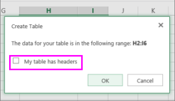
In the Create Table dialog box, you can choose whether your table has headers.
-
Select My table has headers to turn the top row of your data into table headers. The data in this row won’t be filtered.
-
Don’t select the check box if you want Excel for the web to add placeholder headers (that you can rename) above your table data.
-
-
Click OK.
-
To apply a filter, click the arrow in the column header, and pick a filter option.
Filter a range of data
If you don’t want to format your data as a table, you can also apply filters to a range of data.
-
Select the data you want to filter. For best results, the columns should have headings.
-
On the Data tab, choose Filter.
Filtering options for tables or ranges
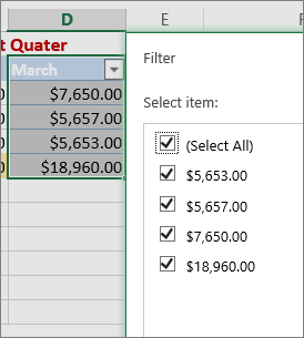
You can either apply a general Filter option or a custom filter specific to the data type. For example, when filtering numbers, you’ll see Number Filters, for dates you’ll see Date Filters, and for text you’ll see Text Filters. The general filter option lets you select the data you want to see from a list of existing data like this:
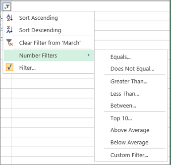
Number Filters lets you apply a custom filter:
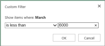
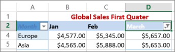
In this example, if you want to see the regions that had sales below $6,000 in March, you can apply a custom filter:
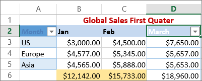
Here’s how:
-
Click the filter arrow next to March > Number Filters > Less Than and enter 6000.
-
Click OK.
Excel for the web applies the filter and shows only the regions with sales below $6000.
You can apply custom Date Filters and Text Filters in a similar manner.
To clear a filter from a column
-
Click the Filter
button next to the column heading, and then click Clear Filter from <«Column Name»>.
To remove all the filters from a table or range
-
Select any cell inside your table or range and, on the Data tab, click the Filter button.
This will remove the filters from all the columns in your table or range and show all your data.
-
Click a cell in the range or table that you want to filter.
-
On the Data tab, click Filter.
-
Click the arrow
in the column that contains the content that you want to filter. -
Under Filter, click Choose One, and then enter your filter criteria.

 in the column that contains the content that you want to filter.
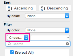
Notes:
-
You can apply filters to only one range of cells on a sheet at a time.
-
When you apply a filter to a column, the only filters available for other columns are the values visible in the currently filtered range.
-
Only the first 10,000 unique entries in a list appear in the filter window.
-
Click a cell in the range or table that you want to filter.
-
On the Data tab, click Filter.
-
Click the arrow
in the column that contains the content that you want to filter. -
Under Filter, click Choose One, and then enter your filter criteria.
-
In the box next to the pop-up menu, enter the number that you want to use.
-
Depending on your choice, you may be offered additional criteria to select:
Notes:
-
You can apply filters to only one range of cells on a sheet at a time.
-
When you apply a filter to a column, the only filters available for other columns are the values visible in the currently filtered range.
-
Only the first 10,000 unique entries in a list appear in the filter window.
-
Instead of filtering, you can use conditional formatting to make the top or bottom numbers stand out clearly in your data.
You can quickly filter data based on visual criteria, such as font color, cell color, or icon sets. And you can filter whether you have formatted cells, applied cell styles, or used conditional formatting.
-
In a range of cells or a table column, click a cell that contains the cell color, font color, or icon that you want to filter by.
-
On the Data tab, click Filter .
-
Click the arrow
in the column that contains the content that you want to filter. -
Under Filter, in the By color pop-up menu, select Cell Color, Font Color, or Cell Icon, and then click a color.
 in the column that contains the content that you want to filter.
This option is available only if the column that you want to filter contains a blank cell.
-
Click a cell in the range or table that you want to filter.
-
On the Data toolbar, click Filter.
-
Click the arrow
in the column that contains the content that you want to filter. -
In the (Select All) area, scroll down and select the (Blanks) check box.
Notes:
-
You can apply filters to only one range of cells on a sheet at a time.
-
When you apply a filter to a column, the only filters available for other columns are the values visible in the currently filtered range.
-
Only the first 10,000 unique entries in a list appear in the filter window.
-
-
Click a cell in the range or table that you want to filter.
-
On the Data tab, click Filter .
-
Click the arrow
in the column that contains the content that you want to filter. -
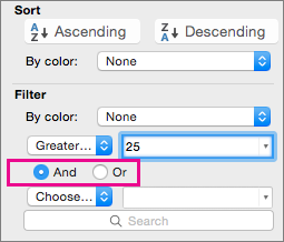
Under Filter, click Choose One, and then in the pop-up menu, do one of the following:
To filter the range for
Click
Rows that contain specific text
Contains or Equals.
Rows that do not contain specific text
Does Not Contain or Does Not Equal.
-
In the box next to the pop-up menu, enter the text that you want to use.
-
Depending on your choice, you may be offered additional criteria to select:
To
Click
Filter the table column or selection so that both criteria must be true
And.
Filter the table column or selection so that either or both criteria can be true
Or.
-
Click a cell in the range or table that you want to filter.
-
On the Data toolbar, click Filter .
-
Click the arrow
in the column that contains the content that you want to filter. -
Under Filter, click Choose One, and then in the pop-up menu, do one of the following:
To filter for
Click
The beginning of a line of text
Begins With.
The end of a line of text
Ends With.
Cells that contain text but do not begin with letters
Does Not Begin With.
Cells that contain text but do not end with letters
Does Not End With.
-
In the box next to the pop-up menu, enter the text that you want to use.
-
Depending on your choice, you may be offered additional criteria to select:
To
Click
Filter the table column or selection so that both criteria must be true
And.
Filter the table column or selection so that either or both criteria can be true
Or.
Wildcard characters can be used to help you build criteria.
-
Click a cell in the range or table that you want to filter.
-
On the Data toolbar, click Filter.
-
Click the arrow
in the column that contains the content that you want to filter. -
Under Filter, click Choose One, and select any option.
-
In the text box, type your criteria and include a wildcard character.
For example, if you wanted your filter to catch both the word «seat» and «seam», type sea?.
-
Do one of the following:
Use
To find
? (question mark)
Any single character
For example, sm?th finds «smith» and «smyth»
* (asterisk)
Any number of characters
For example, *east finds «Northeast» and «Southeast»
~ (tilde)
A question mark or an asterisk
For example, there~? finds «there?»
Do any of the following:
|
To |
Do this |
|---|---|
|
Remove specific filter criteria for a filter |
Click the arrow |
|
Remove all filters that are applied to a range or table |
Select the columns of the range or table that have filters applied, and then on the Data tab, click Filter. |
|
Remove filter arrows from or reapply filter arrows to a range or table |
Select the columns of the range or table that have filters applied, and then on the Data tab, click Filter. |
When you filter data, only the data that meets your criteria appears. The data that doesn’t meet that criteria is hidden. After you filter data, you can copy, find, edit, format, chart, and print the subset of filtered data.
Table with Top 4 Items filter applied
Filters are additive. This means that each additional filter is based on the current filter and further reduces the subset of data. You can make complex filters by filtering on more than one value, more than one format, or more than one criteria. For example, you can filter on all numbers greater than 5 that are also below average. But some filters (top and bottom ten, above and below average) are based on the original range of cells. For example, when you filter the top ten values, you’ll see the top ten values of the whole list, not the top ten values of the subset of the last filter.
In Excel, you can create three kinds of filters: by values, by a format, or by criteria. But each of these filter types is mutually exclusive. For example, you can filter by cell color or by a list of numbers, but not by both. You can filter by icon or by a custom filter, but not by both.
Filters hide extraneous data. In this manner, you can concentrate on just what you want to see. In contrast, when you sort data, the data is rearranged into some order. For more information about sorting, see Sort a list of data.
When you filter, consider the following guidelines:
-
Only the first 10,000 unique entries in a list appear in the filter window.
-
You can filter by more than one column. When you apply a filter to a column, the only filters available for other columns are the values visible in the currently filtered range.
-
You can apply filters to only one range of cells on a sheet at a time.
Note: When you use Find to search filtered data, only the data that is displayed is searched; data that is not displayed is not searched. To search all the data, clear all filters.
Need more help?
You can always ask an expert in the Excel Tech Community or get support in the Answers community.
Filter a range of data Select any cell within the range. Select Data > Filter. Select Text Filters or Number Filters, and then select a comparison, like Between. Enter the filter criteria and select OK.
Contents
- 1 Is it possible to filter rows in Excel?
- 2 Can you filter multiple rows in Excel?
- 3 How do I filter rows by list in Excel?
- 4 How do I filter rows in sheets?
- 5 Why is Excel only filtering some rows?
- 6 How do I filter rows in Excel with certain text?
- 7 How do I group rows in Excel?
- 8 What is the difference between filter and advanced filter?
- 9 How do you filter rows based on a list selection in another sheet?
- 10 How do I select a list of rows in Excel?
- 11 What is an Xlookup in Excel?
- 12 Can you filter a spreadsheet horizontally?
- 13 Can you filter Google sheets by row?
- 14 How do I filter in Excel and keep rows together?
- 15 How do you filter in Excel and keep rows together?
- 16 How do I sort multiple rows horizontally in Excel?
- 17 How do I highlight all rows with specific text?
- 18 How do you club multiple rows in Excel?
- 19 How do I create multiple groups of rows in Excel?
- 20 How do I filter the third row in Excel?
Is it possible to filter rows in Excel?
You can filter rows and columns to select which rows or columns to display in the form.Right-click a row or column member, select Filter, and then Filter. In the left-most field in the Filter dialog box, select the filter type: Keep: Include rows or columns that meet the filter criteria.
Can you filter multiple rows in Excel?
Excel’s advanced filter is flexible. You can include multiple columns and rows in the filter. Keep in mind that values in the same row find records where both criteria values are found; criteria values in different rows displays records where either value is found.
How do I filter rows by list in Excel?
To run the Advanced Filter:
- Select a cell in the data table.
- On the Data tab of the Ribbon, in the Sort & Filter group, click Advanced.
- For Action, select Filter the list, in-place.
- For List range, select the data table.
- For Criteria range, select C1:C2 – the criteria heading and formula cells.
- Click OK, to see the results.
How do I filter rows in sheets?
Filter your data
- On your computer, open a spreadsheet in Google Sheets.
- Select a range of cells.
- Click Data. Create a filter.
- To see filter options, go to the top of the range and click Filter . Filter by condition: Choose conditions or write your own.
- To turn the filter off, click Data. Remove filter.
Why is Excel only filtering some rows?
1. Check that you have selected all of the data. If your data has empty rows and/or columns or if you are only wanting to filter a specific range, select the area you want to filter prior to turning Filter on. Failing to select the area leaves Excel to set the filter area.
How do I filter rows in Excel with certain text?
- Select the Data tab, then click the Filter command. A drop-down arrow will appear in the header cell for each column.
- Click the drop-down arrow for the column you want to filter.
- The Filter menu will appear.
- The Custom AutoFilter dialog box will appear.
- The data will be filtered by the selected text filter.
How do I group rows in Excel?
To group rows or columns:
- Select the rows or columns you want to group. In this example, we’ll select columns A, B, and C.
- Select the Data tab on the Ribbon, then click the Group command. Clicking the Group command.
- The selected rows or columns will be grouped. In our example, columns A, B, and C are grouped together.
What is the difference between filter and advanced filter?
Here are some differences between the regular filter and Advanced filter: While the regular data filter will filter the existing dataset, you can use Excel advanced filter to extract the data set to some other location as well. Excel Advanced Filter allows you to use complex criteria.
How do you filter rows based on a list selection in another sheet?
Step 1: Select data you want to do filter, in this case we select A2:C11, select Data->Advanced. Step 2: On Advanced Filter dialog, check on ‘Filter the list, in-place’, in List range select $A$2:$A$11, in Criteria range, select $F$2:$F$6. Then click OK. Step 3: After above steps, names are filtered properly.
How do I select a list of rows in Excel?
Select one or more rows and columns
Or click on any cell in the column and then press Ctrl + Space. Select the row number to select the entire row. Or click on any cell in the row and then press Shift + Space. To select non-adjacent rows or columns, hold Ctrl and select the row or column numbers.
What is an Xlookup in Excel?
Use the XLOOKUP function to find things in a table or range by row.With XLOOKUP, you can look in one column for a search term, and return a result from the same row in another column, regardless of which side the return column is on.
Can you filter a spreadsheet horizontally?
With a slight adjustment to your references in the filter formula, you can filter horizontally, where you are filtering columns instead of rows.
Can you filter Google sheets by row?
Click Z->A to sort the rows from greatest to least based on the contents of this column.If you select Filter by condition, you can create rules that will instruct the Sheet to automatically filter out rows that contain certain results.
How do I filter in Excel and keep rows together?
To do this, use Excel’s Freeze Panes function. If you want to freeze just one row, one column or both, click the View tab, then Freeze Panes. Click either Freeze First Column or Freeze First Row to freeze the appropriate section of your data. If you want to freeze both a row and a column, use both options.
How do you filter in Excel and keep rows together?
Then in the Ribbon, go to Home > Sort & Filter > Sort Largest to Smallest. 2. In the Sort Warning window, select Expand the selection, and click Sort. Along with Column G, the rest of the columns will also be sorted, so all rows are kept together.
How do I sort multiple rows horizontally in Excel?
Sort Multiple Rows Horizontally
- Select the data range that we want to sort (B3:G4), and in the Ribbon, go to Home > Sort & Filter > Custom Sort.
- In the Sort window, click Add Level, to add Row 4 to the sort condition.
- In the second level, select Row 4 for Then by, and Largest to Smallest for Order, and click OK.
How do I highlight all rows with specific text?
If you want to highlight rows in a table that contain specific text, you use conditional formatting with a formula that returns TRUE when the the text is found. The trick is to concatenate (glue together) the columns you want to search and to lock the column references so that only the rows can change.
How do you club multiple rows in Excel?
To merge two or more rows into one, here’s what you need to do:
- Select the range of cells where you want to merge rows.
- Go to the Ablebits Data tab > Merge group, click the Merge Cells arrow, and then click Merge Rows into One.
How do I create multiple groups of rows in Excel?
Select the data (including any summary rows or columns). On the Data tab, in the Outline group, click Group > Group Rows or Group Columns. Optionally, if you want to outline an inner, nested group — select the rows or columns within the outlined data range, and repeat step 3.
How do I filter the third row in Excel?
Step 1 Highlight the bottom header row. and then You can select just the cells in a row, or select the entire row. Step 2 next click on “Sort & Filter” on the Home tab, then you can select “Filter.” Excel adds filter arrows to all the column names.
This tutorial demonstrates how to filter rows in Excel and Google Sheets.
Excel enables you to store data in a table format made up of rows and columns. These tables are often in database format with the columns as the headers (database fields), and the rows as the database entries. Excel then has some fabulous database features, one of which is the ability to filter lists of data. Filtering data lists enables you to locate and report on a subset of the data.
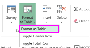
Format Data as a Table
Once you have a list of data stored in Excel, you can choose to format the data as a table. Doing this automatically adds filters to the columns in the table.
- Click in the data, and then in the Ribbon, go to Home > Styles > Format as Table. Select the type of format you wish to apply.
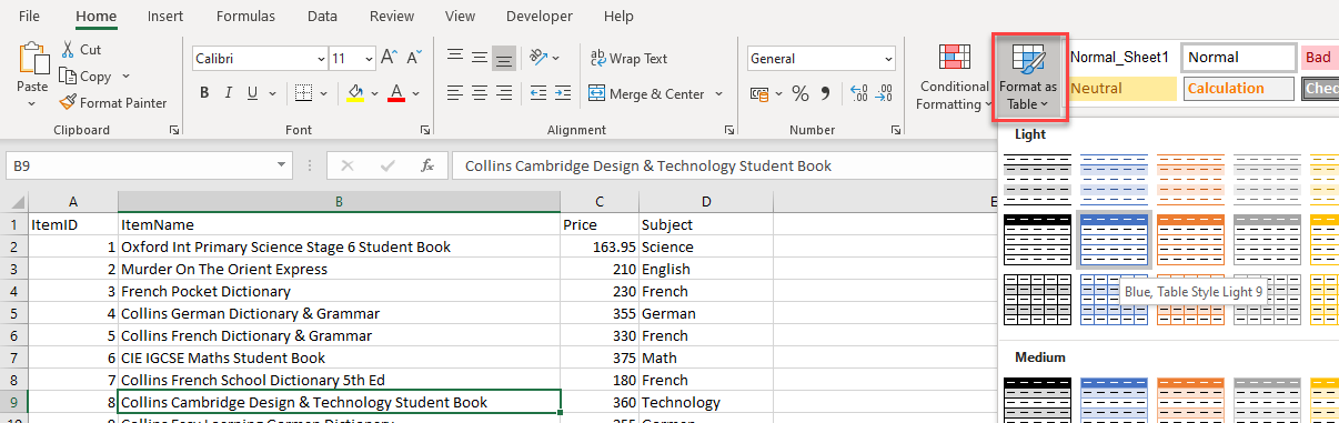
- In the Format As Table dialog box, check My table has headers (if it isn’t checked already).
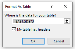
The format is applied to the data, and a new tab called Table Design appears in your Ribbon.
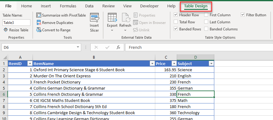
Add Filter to Excel Data
If you do not format your data as a table, you can still add filters to the data manually.
▸ Click in your data, and then, in the Ribbon, go to Home > Editing > Filter.
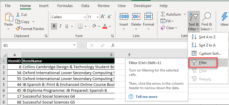
Small drop-down arrows (filter buttons) are applied to the header row of your data.
Tip: The shortcut to apply an AutoFilter is CTRL + SHIFT + L.
Filter by Column With Filter Arrows
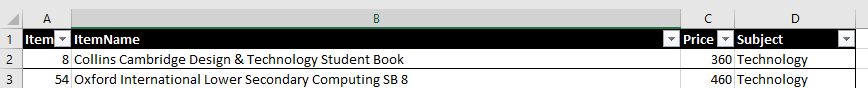
- Click on the drop-down arrow to the right of the heading you wish to filter on, and then remove the checkmark from Select all.
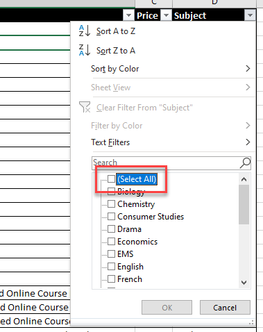
- In the list of entries that is shown, click in the checkbox of the ones that you need to be shown in your filtered data.
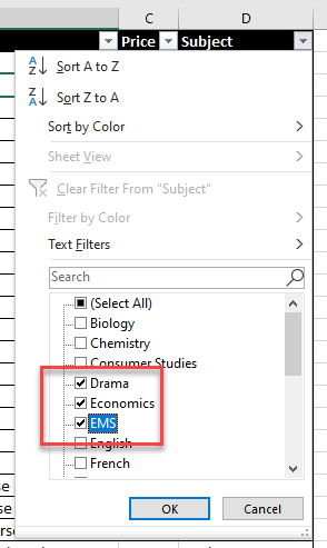
- Click OK to show the data.
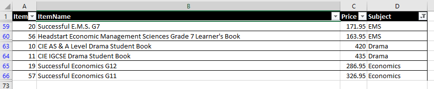
Notice that the data that does not match what you have selected is hidden – the row headers turn blue as only the rows for the filtered data are shown. Also, the header that you have filtered on has a small icon of a filter indicating that that column of data has the filter applied to it.
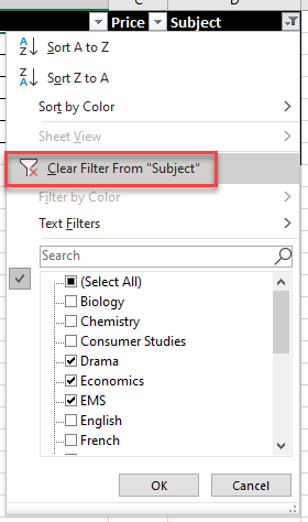
Clear Filter
Click on the small filter to activate the drop-down list. Go to Clear Filter From “Subject“ to remove the filter from the data.
OR
Check (Select All) and then click OK to remove the filter from the data.
OR
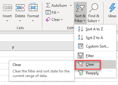
In the Ribbon, go to Home > Editing > Filter > Clear.
This will clear the filter from the data, but the filter headers will still remain at the top of each column of data.
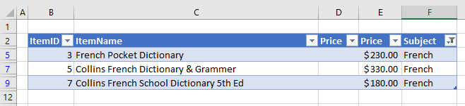
Filter by Text
- Click on the drop-down arrow next to the header column of the data you wish to filter, and then click Text Filters.
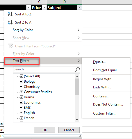
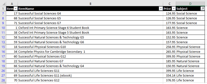
- Select Contains… from the list shown and then type in a word that is contained within the data, e.g., Science.
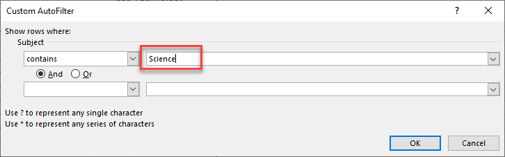
- Click OK to filter the data.
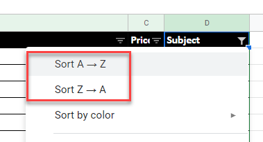
Sort Filter
The filter drop-down list has the ability to sort the filtered data.
In the filter drop-down list, click Sort A to Z or Sort Z to A, depending on how you wish to sort the filtered data.
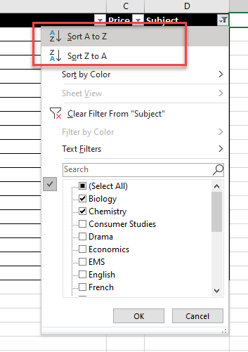
The data that is filtered is sorted – you will notice a small arrow appearing next to the filter, indicating that the filtered data is sorted.
If you remove the filter, you will notice that the rest of the data in the list has not been sorted.
To sort the entire list of data, once the filter is cleared, you can click Sort A to Z or Sort Z to A in the filter drop-down list.
OR
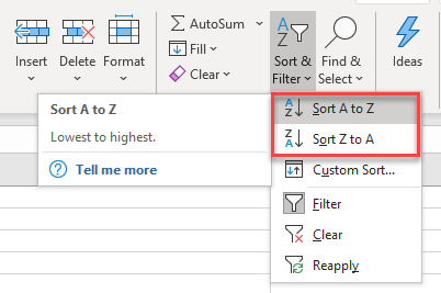
In the Ribbon, go to Home > Editing > Sort & Filter and then click Sort A to Z or Sort Z to A.
Remove Filters
To remove the filters from the data list, in the Ribbon, go to Home > Editing > Sort & Filter and then click on Filter once again. This is a toggle button so will either apply filters to the list, or remove filters from the list.
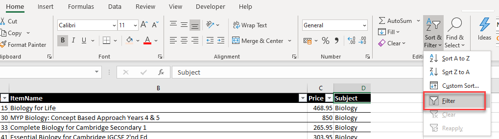
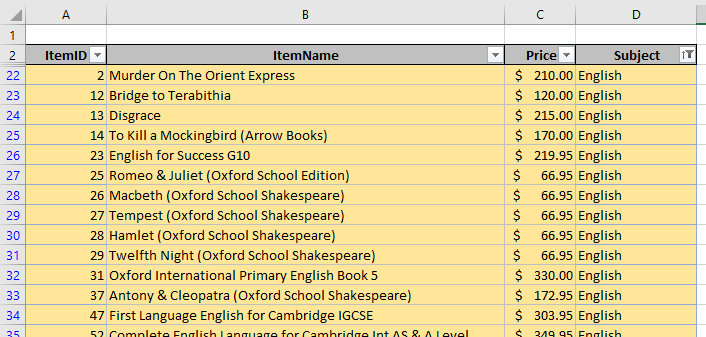
Filter by Color
If you have formatted your data by color, Excel has the ability to filter the data based on the colors applied.
- In the filter drop down, go to Filter by Color.
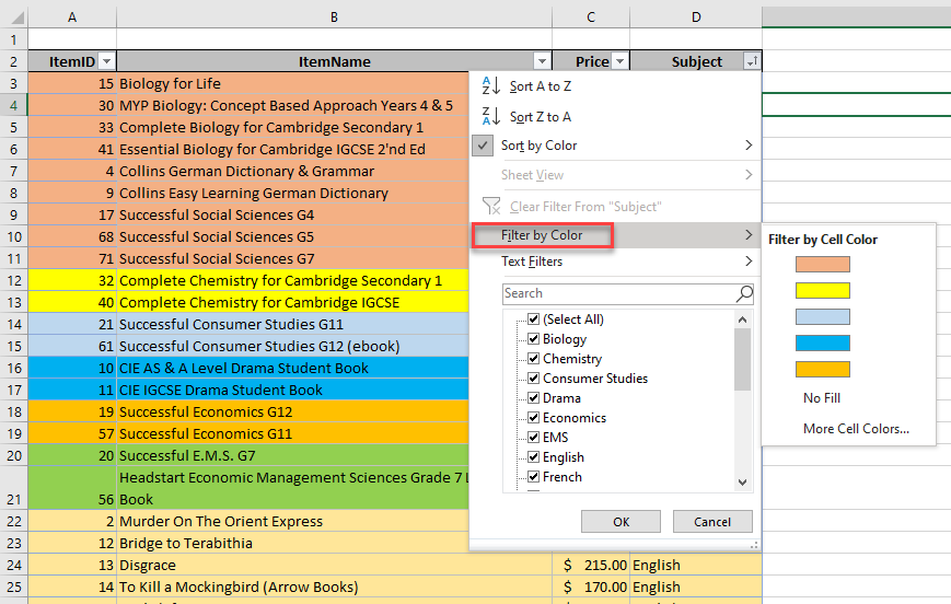
- Select More Cell Colors to see all the cell colors applied to the data.
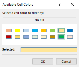
- Select the color you wish to filter on, and then click OK.
Filter Rows in Google Sheets
The processes for filtering data in Google Sheets and Excel are similar. The main difference is how items are selected.
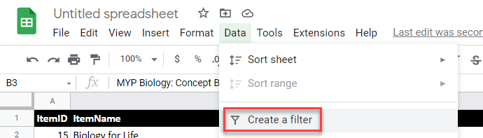
- In the Menu, go to Data > Create a Filter.
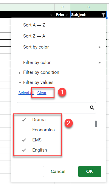
- In the drop-down list, click Clear to clear all the checkmarks from the data, and then tick the data items from the list.
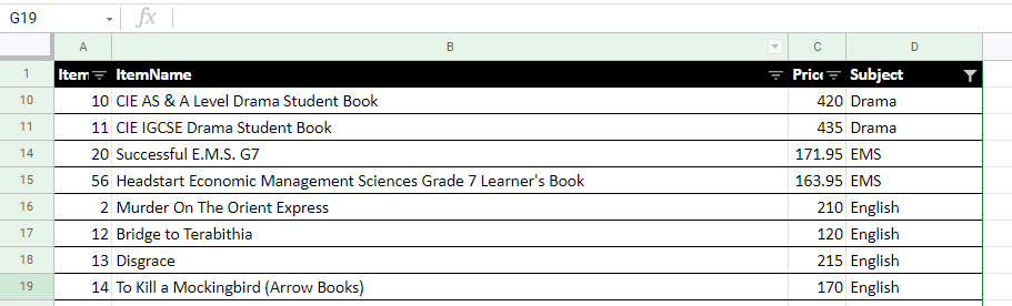
- Click OK to filter the data.
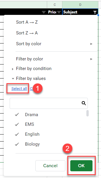
To remove the filter, in the drop-down list, click Select All and then click OK.
The filter is cleared but the filter drop down will still be showing on the column headers.
Filter for Specific Text
- To filter the data by specific text, click Filter by condition and then in the drop down below, choose Text contains. There are multiple conditions that you are able to filter on.
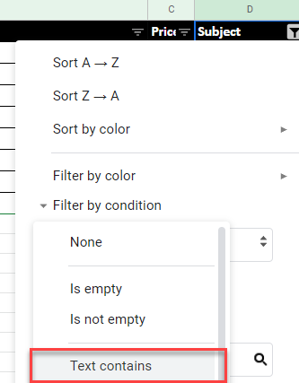
- Type in the text that you wish to filter on, and then click OK.
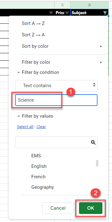
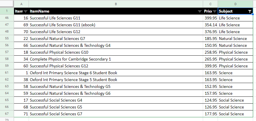
Only the rows that contain the relevant data are shown.
Once you have filtered the data, you can also sort the data as you can in Excel.
In the filter drop-down list, click Sort A to Z or Sort Z to A, depending on how you wish to sort the filtered data.
Note that as with Excel, this will only sort the filtered data – not the entire data list.
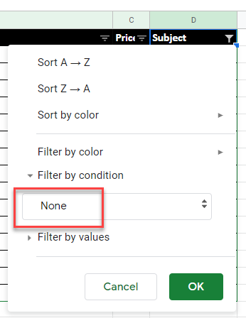
To remove the filter, go to Filter by condition > None in filter the drop-down list, and then click OK.
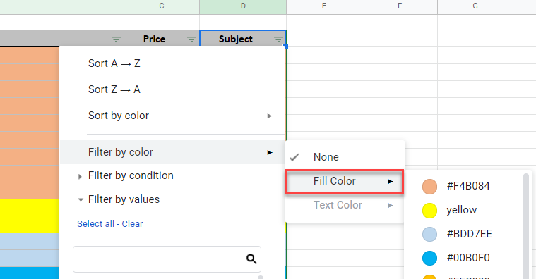
You can also filter by color in Google Sheets.
In the drop-down filter list, go to Filter by color > Fill color and then choose one of the fill colors shown.
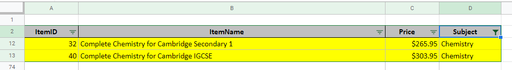
The data is filtered by the chosen color.
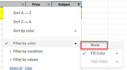
To remove the filter, go to Filter by color > None in the drop-down filter list.
Advanced filter in Excel provides more opportunities for managing on data management spreadsheets. It is more complex in settings, but much more effective in action.
Using a standard filter, a Microsoft Excel user can solve not all of the tasks that are set. There is no visual display of the applied filtering conditions. It is not possible to apply more than two selection criteria. You can not filter the duplicate values to leave only unique records. And the criteria themselves are schematic and simple. The functionality of the extended filter is much richer. Let’s take a closer look at its possibilities.
How to make the advanced filter in Excel?
The advanced filter allows you to analysis data on an unlimited set of conditions. With this tool, the user can:
- to specify more than two selection criteria;
- to copy the result of filtering to another sheet;
- to set the condition of any complexity with the helping of formulas;
- to extract the unique values.
The algorithm for applying the extended filter is simple.
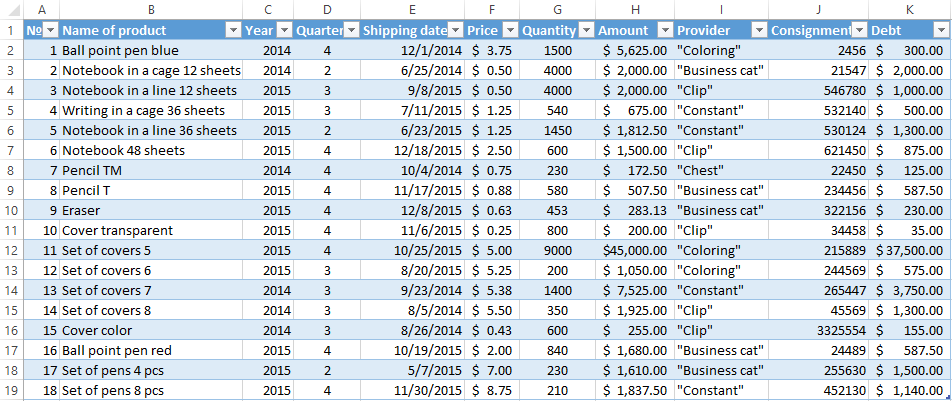
- To make the table with the original data or to open an existing one. Like so:
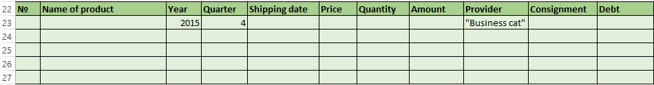
- To create the condition table. The features: the header line is the same with the «cap» of the filtered table. To avoid errors, need to copy the header line in the source table and paste it on the same sheet (side, top, underarm) or on another sheet. We enter the selection criteria into the condition table.
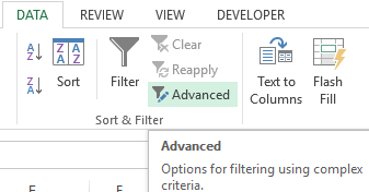
- Go to the «DATA» tab — «Sort and filter» — «Advanced». If the filtered information should be displayed on another sheet (NOT where the source table is), then you need to run the extended filter from another sheet.
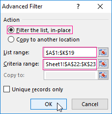
- In the «Advanced Filter» window that opens, to select the method of processing information (on the same sheet or on the other one), set the initial range (the table 1, example) and the range of conditions (the table 2, conditions). The header lines must be included in the ranges.
- To close the «Advanced Filter» window, click OK. We see the result.

The top table is the result of the filtering. The lower nameplate with the conditions is given for clarity near.
How to use the advanced filter in Excel?
To cancel the action of the advanced filter, we place the cursor anywhere in the table and press Ctrl + Shift + L or «DATA» — «Sort and Filter» — «Clear».
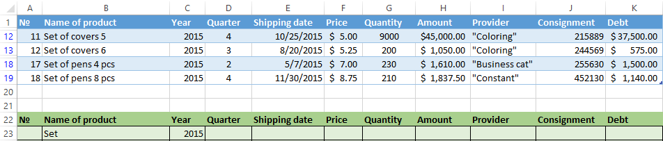
We will find using the «Advanced Filter» tool information on the values that contain the word «Set».
In the table of conditions we bring in the criteria. For example, these are:

The program in this case will search for all information on the goods, in the title of which there is the word «Set».
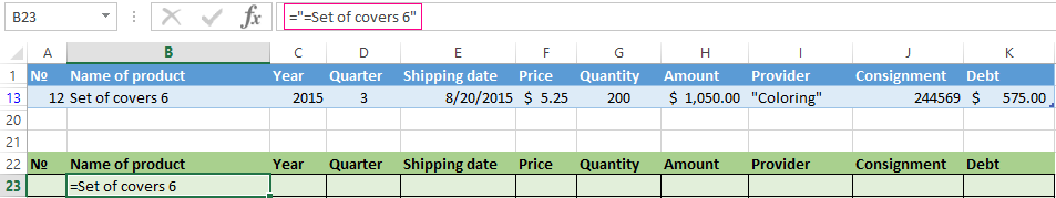
To search for the exact value, you can use the «=» sign. We enter the following criteria in the condition table:

Excel sees the «=» as a signal: the user will set the formula now. In order for the program to work correctly, the following should be written in the formula line: =»=Set of covers 6″.
After using the «Advanced Filter»:
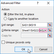
We filter the source table by the condition «OR» for different columns now. The operator «OR» is also in the tool «AutoFilter». But there it can be used within the single column.
In the condition label we introduce the selection criteria: =»=Set of covers 6″. (In the column «Name of product») and = «<2.5$» (in the column «Price»). That is, the program must select those values that contain the EXACTLY information about the good «Set of covers 6 ». OR to the information about the goods, which price is <2.5.

Please note: the criteria must be written under the corresponding headings in the DIFFERENT lines.
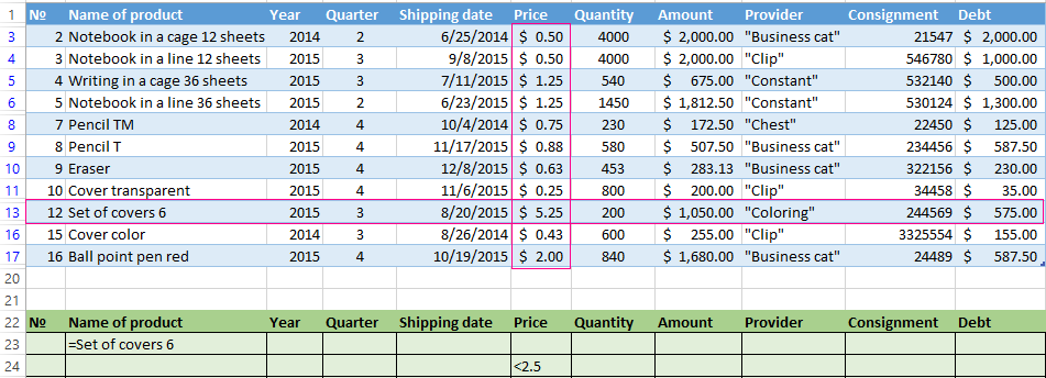
The result of selection:
The advanced filter allows you to use as a criterion of a formula. Let’s consider the example.

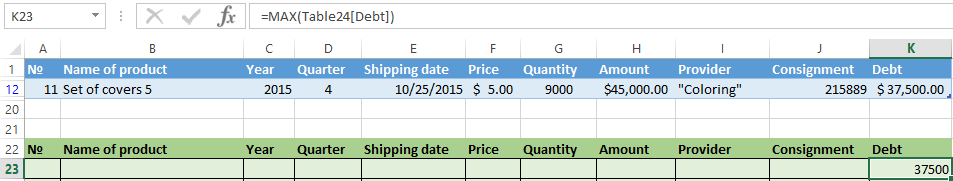
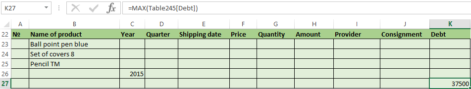
Selection of the line with the maximum indebtedness: =MAX(Table1[Debt]).
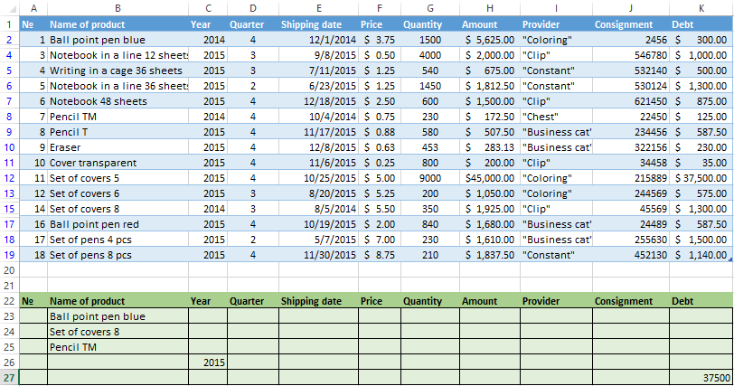
So we get the results as after running several filters on the one Excel sheet.
How to make few filters in Excel?
Let’s create the filter by several values. To do this, we enter in the table of conditions several criteria for selecting data:
Apply the tool «Advanced Filter»:
Now from the table with the selected data we will extract new information, which was selected according to other criteria. There are only shipping date for autumn 2015 (from September to November). Example:
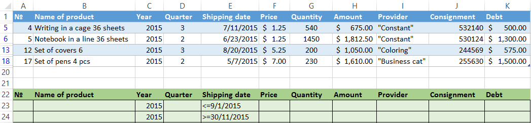
We introduce a new criterion in the condition table and apply the filtering tool. The initial range — is the table with data selected according to the previous criterion. This is how the filter is performed across on several columns.
To use few filters, you can create several condition tables on the new sheets. The method of implementation depends from the task which was set by user.
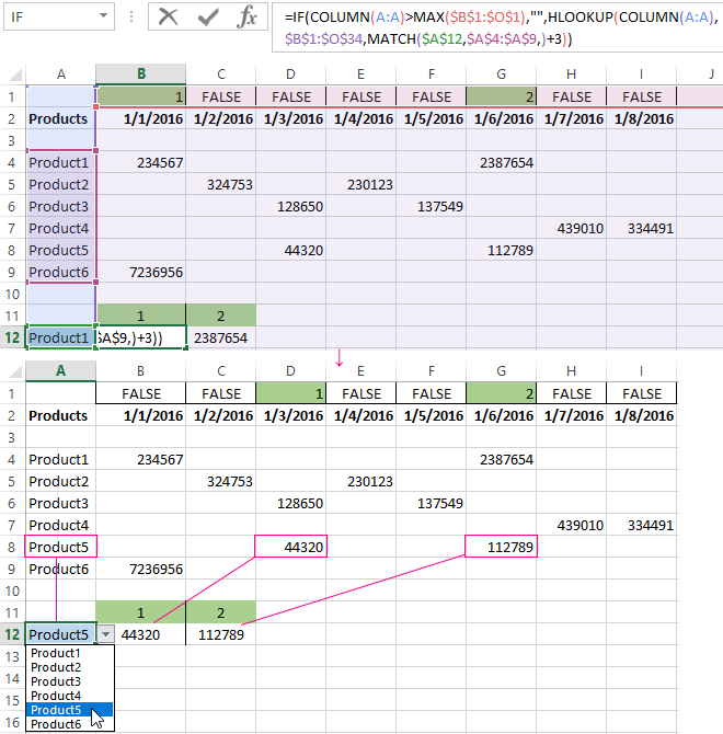
How to make the filter in Excel by lines?
By standard methods — you may not do it by any ways. Microsoft Excel selects data only in columns. Therefore, we need to look for other solutions.
Here are some examples of string criteria for the extended filter in Excel:
- Convert to the table. For example, from three rows make a list of three columns and apply the filtering to the transformed version.
- Use formulas to display exactly the data in the string that are needed. For example, make some indicator drop-down list. And in the next cell, enter the formula using the IF function. When a certain value is selected from the drop-down list, its parameter appears next to it.
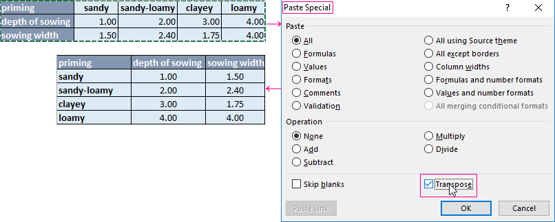
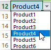
To give an example of how the filter works by rows in Excel, we are creating the label:
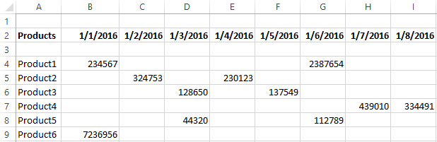
For the list of products, we create the drop-down list:
If necessary, learn how to create a drop-down list in Excel.
Above the table with the original data, we insert an empty line. In the cells, we introduce the formula that will show which columns the information is taken from.
Next to the drop-down list box, we enter the following formula:
Its task is select from the table those values, that correspond to a certain good.
Download examples of advanced filtering
Thus, using the tool «Drop-down list» and built-in functions Excel selects data in rows according to a certain criterion.
Note: FILTER is a new dynamic array function in Excel 365. In other versions of Excel, there are alternatives, but they are more complex.
In this example, the goal is to filter the data shown in B5:G15 by year, then sort the results in descending order. In addition, the result should include the Group column, sorted in the same way. The problem breaks down into two main steps:
- Filter to select the Group and matching Year column
- Sort the result in descending order by year values
Filter by column
To filter the data to select the Group column and data for the matching year, we use the FILTER function. Typically FILTER is used to filter data vertically, selecting rows that match provided conditions. However, FILTER can also select data horizontally. The key is to provide logic for the include argument that will return a horizontal array with the same number of columns as the source data. For example, to return data for the year 2017, we can use a formula like this:
=FILTER(B5:G15,B4:G4=2017)
The logical expression:
=B4:G4=2017
returns a one-row horizontal array with 5 columns:
{FALSE,FALSE,TRUE,FALSE,FALSE,FALSE}
When provided to FILTER as the include argument, FILTER returns the values for 2017 only:
FILTER(B5:G15,{FALSE,FALSE,TRUE,FALSE,FALSE,FALSE}) // 2017 only
To add in the Group column, we extend the logic using Boolean logic, a technique for working with TRUE and FALSE values as 1s and 0s. In Boolean algebra, multiplication corresponds to AND logic, and addition corresponds to OR logic. In this case, we want FILTER to return the Group column and the matching year column. This means we need OR logic — i.e. column = «group» OR column = [year].
Using addition for OR logic, we can construct an expression like this:
=(B4:G4="group")+(B4:G4=2017)
This results in two arrays with TRUE and FALSE values, joined by addition:
{TRUE,FALSE,FALSE,FALSE,FALSE,FALSE} +
{FALSE,FALSE,TRUE,FALSE,FALSE,FALSE}
The math operation of addition coerces the TRUE and FALSE to numbers, and the result is a single array of 1s and 0s:
{1,0,1,0,0,0}
Notice the first and third columns are 1, while the other columns are 0. When this array is provided to FILTER as the include argument, FILTER returns columns 1 and 3 from the data.
Sort by row
Because the FILTER function is nested inside the SORT function. FILTER returns the two matching columns explained above directly to SORT:
=SORT(filter_result,2,-1)
We want to sort these columns by values in the year column (2017) in descending order, so sort_index is provided as 2, and sort_order is given as -1. With these inputs, the SORT function returns the sorted as shown in the example. Notice that Group E appears first since 27% is the highest value in 2017.
When the year in J4 is changed, FILTER selects new columns, and the SORT function sorts the new data in the same way.
Dropdown menu for year
To make the year dropdown menu, you can apply a simple data validation rule to cell J4. The allowed values are based on the existing years in C4:G4, with In-cell dropdown selected:

Once data validation is in place, a dropdown menu with the years 2016-2020 will appear. If you are new to data validation, see our Data Validation Guide.