
To generate descriptive statistics for these scores, execute the following steps.
- On the Data tab, in the Analysis group, click Data Analysis.
- Select Descriptive Statistics and click OK.
- Select the range A2:A15 as the Input Range.
- Select cell C1 as the Output Range.
- Make sure Summary statistics is checked.
- Click OK.
Contents
- 1 How do you do descriptive statistics in Excel 2021?
- 2 How do I get all statistics in Excel?
- 3 How do you do descriptive statistics?
- 4 How do I do descriptive data analysis in Excel?
- 5 What is Excel descriptive statistics?
- 6 How can descriptive statistics be used to summarize data?
- 7 How do you report descriptive statistics?
- 8 What are the 3 types of statistics?
- 9 What are the 5 descriptive statistics?
- 10 Which type of statistics summarize variables in a data set?
- 11 How do you explain summary statistics?
- 12 What do Summary statistics tell you?
- 13 What are the 8 descriptive statistics?
- 14 What are the four types of descriptive statistics?
- 15 What does N mean in statistics?
- 16 How does SPSS calculate descriptive statistics?
- 17 What are example of statistics?
- 18 What is the 2 types of statistics?
- 19 How do you write a five-number summary?
- 20 What are the 5 types of variables?
How do you do descriptive statistics in Excel 2021?
Go to the Data tab > Analysis group > Data analysis. Select Descriptive Statistics and click OK.
Descriptive Statistics
- Select the range of your input.
- Select the range from where you want to display the output.
- Check the summary statistics.
How do I get all statistics in Excel?
Click the Data tab’s Data Analysis command button to tell Excel that you want to calculate descriptive statistics. Excel displays the Data Analysis dialog box. In the Data Analysis dialog box, highlight the Descriptive Statistics entry in the Analysis Tools list and then click OK.
How do you do descriptive statistics?
Descriptive statistics are used to describe the basic features of the data in a study.
For example, you could use percentages to describe the:
- percentage of people in different income levels.
- percentage of people in different age ranges.
- percentage of people in different ranges of standardized test scores.
How do I do descriptive data analysis in Excel?
In This Article
- Click the Data tab’s Data Analysis command button to tell Excel that you want to calculate descriptive statistics.
- In the Data Analysis dialog box, highlight the Descriptive Statistics entry in the Analysis Tools list and then click OK.
What is Excel descriptive statistics?
Excel Descriptive Statistics
Using the descriptive statistics feature in Excel means that you won’t have to type in individual functions like MEAN or MODE. One button click will return a dozen different stats for your data set.
How can descriptive statistics be used to summarize data?
Interpret the key results for Descriptive Statistics
- Step 1: Describe the size of your sample.
- Step 2: Describe the center of your data.
- Step 3: Describe the spread of your data.
- Step 4: Assess the shape and spread of your data distribution.
- Compare data from different groups.
How do you report descriptive statistics?
Descriptive Results
- Add a table of the raw data in the appendix.
- Include a table with the appropriate descriptive statistics e.g. the mean, mode, median, and standard deviation.
- Identify the level or data.
- Include a graph.
- Give an explanation of your statistic in a short paragraph.
What are the 3 types of statistics?
Types of Statistics
- Descriptive statistics.
- Inferential statistics.
What are the 5 descriptive statistics?
There are a variety of descriptive statistics. Numbers such as the mean, median, mode, skewness, kurtosis, standard deviation, first quartile and third quartile, to name a few, each tell us something about our data.
Which type of statistics summarize variables in a data set?
Descriptive statistics are used to describe or summarize the characteristics of a sample or data set, such as a variable’s mean, standard deviation, or frequency. Inferential statistics can help us understand the collective properties of the elements of a data sample.
How do you explain summary statistics?
Summary statistics summarize and provide information about your sample data. It tells you something about the values in your data set. This includes where the mean lies and whether your data is skewed.
What do Summary statistics tell you?
The information that gives a quick and simple description of the data. Can include mean, median, mode, minimum value, maximum value, range, standard deviation, etc.
What are the 8 descriptive statistics?
In this article, the first one, you’ll find the usual descriptive statistics concepts: Measures of Central Tendency: Mean, Median, Mode. Measures of Dispersion: Variance and Standard Deviation. Measures of Position: Quartiles, Quantiles and Interquartiles.
What are the four types of descriptive statistics?
There are four major types of descriptive statistics:
- Measures of Frequency: * Count, Percent, Frequency.
- Measures of Central Tendency. * Mean, Median, and Mode.
- Measures of Dispersion or Variation. * Range, Variance, Standard Deviation.
- Measures of Position. * Percentile Ranks, Quartile Ranks.
What does N mean in statistics?
The symbol ‘N’ represents the total number of individuals or cases in the population.
How does SPSS calculate descriptive statistics?
Using the Descriptives Dialog Window
- Click Analyze > Descriptive Statistics > Descriptives.
- Add the variables English , Reading , Math , and Writing to the Variables box.
- Check the box Save standardized values as variables.
- Click OK when finished.
What are example of statistics?
A statistic is a number that represents a property of the sample. For example, if we consider one math class to be a sample of the population of all math classes, then the average number of points earned by students in that one math class at the end of the term is an example of a statistic.
What is the 2 types of statistics?
The two major areas of statistics are known as descriptive statistics, which describes the properties of sample and population data, and inferential statistics, which uses those properties to test hypotheses and draw conclusions.
How do you write a five-number summary?
How to Find a Five-Number Summary: Steps
- Step 1: Put your numbers in ascending order (from smallest to largest).
- Step 2: Find the minimum and maximum for your data set.
- Step 3: Find the median.
- Step 4: Place parentheses around the numbers above and below the median.
- Step 5: Find Q1 and Q3.
What are the 5 types of variables?
There are different types of variables and having their influence differently in a study viz. Independent & dependent variables, Active and attribute variables, Continuous, discrete and categorical variable, Extraneous variables and Demographic variables.
In the modern data-driven business world, we have sophisticated software dedicatedly to working towards “Statistical Analysis.” Amidst all these modern, technologically advanced excel software is not a bad tool to do your statistical analysis of the data. Of course, we can do all statistical analysis using Excel, but you should be an advanced Excel user. This article will show you some basic to intermediate-level statistics calculations using Excel.
Table of contents
- Excel Statistics
- How to use Excel Statistical Functions?
- #1: Find Average Sale per Month
- #2: Find Cumulative Total
- #3: Find Percentage Share
- #4: ANOVA Test
- Things to Remember
- Recommended Articles
- How to use Excel Statistical Functions?
How to use Excel Statistical Functions?
You can download this Statistics Excel Template here – Statistics Excel Template
#1: Find Average Sale per Month
The average rate or trend is what the decision-makers look at when they want to make crucial and quick decisions. So finding the average sales, cost, and profit per month is a common task everybody does.
For example, look at the below data of monthly sales value, cost value, and profit value columns in Excel.

So, by finding the average per month from the whole year, we can see what per month numbers are.
Using the AVERAGE functionThe AVERAGE function in Excel gives the arithmetic mean of the supplied set of numeric values. This formula is categorized as a Statistical Function. The average formula is =AVERAGE(read more, we can find the average values from 12 months, which boils down to per month on an average.
- Open the AVERAGE function in the B14 cell.

- Select the values from B2 to B13.

- The average value for sales is:

- Copy and paste cell B14 to the other two cells to get the average cost and profit. The average value for the cost is:

- The average value for the profit is:

So, on average, per month, the sale value is $25,563, the cost value is $24,550, and the profit value is $1,013.
#2: Find Cumulative Total
Finding the cumulative total is another set of calculations in excel statistics. Cumulative is nothing but adding all the previous month’s numbers together to find the current total for the period.
The steps to find the cumulative total are as follows:
- First, look at the below 6 months sales numbers.

- Open the SUM function in the C2 cell.

- Select the cell B2 cell and make the range reference.

From the range of cells, make the first part of the cell reference B2 an absolute reference by pressing the F4 key. - Close the bracket and press the “Enter” key.

- Drag and drop the formula below one cell.

- Now, we have the first two months’ cumulative total. At the end of the first two months, revenue was $53,835. Drag and drop the formula to other remaining cells.

From this cumulative, we can find in which month there was a less revenue increase.


Out of twelve months, you may have got $1,000,000 in revenue. But, still, maybe in one month, you must have achieved the majority of the revenue, and finding the month’s percentage share helps us find the particular month’s percentage share.
For example, look at the below data of the monthly revenue.

To find the percentage share first, we need to see what the overall 12 months total is, so by applying the SUM function in excelThe SUM function in excel adds the numerical values in a range of cells. Being categorized under the Math and Trigonometry function, it is entered by typing “=SUM” followed by the values to be summed. The values supplied to the function can be numbers, cell references or ranges.read more, find the overall sales value.

We can use the formula to find the percentage share of each month.
% Share = Current Month Revenue / Overall Revenue
To apply the formula as B2 / B14.

The percentage share for Jan month is:

Note: Make the overall sales total cell (B14 cell) an absolute referenceAbsolute reference in excel is a type of cell reference in which the cells being referred to do not change, as they did in relative reference. By pressing f4, we can create a formula for absolute referencing.read more because this cell will be a common divisor value across 12 months.
Copy and paste the C2 cell to the below cells as well.

Apply the “Percentage” format to convert the value to percentage values.

So, from the above percentage share, we can identify that the “Jun” month has the highest contribution to overall sales value, i.e., 11.33%, and the “May” month has the lowest contribution to overall sales value, i.e., 5.35%.

#4: ANOVA Test
Analysis of Variance (ANOVA) is the statistical tool in excel used to find the best available alternative from the lot. For example, if you are introducing four new kinds of food to the market. You gave a sample of each food to get the public’s opinion and from the opinion score given by the public by running the ANOVA test. We can choose the best from the lot.
ANOVA is a data analysis tool available in Excel under the “DATA” tab. By default, it is not available. You need to enable it.

Below are the scores of three students from 6 different subjects.

Click on the “Data Analysis” option under the “Data” tab. It will open up below the “Data Analysis” tab.

Scroll up and choose “Anova: Single Factor.”

Choose “Input Range” as B1 to D7 and tick “Labels in first row.”

Select the “Output Range” as any of the cells in the same worksheet.

We will have an “ANOVA” analysis ready.

Things to Remember
- All the basic and intermediate statistical analyses are possible in Excel.
- We have formulas under the category of “Statistical” formulas.
- If you are from a statistics background, it is easy to do fancy and important statistical analyses in Excel like T-TEST, Z-TEST, Descriptive StatisticsDescriptive statistics is used to summarize information available in statistics, and there is a descriptive statistics function in Excel as well. This built-in tool is found in the data tab, in the data analysis section.read more,” etc.
Recommended Articles
This article is a guide to statistics in excel. Here, we discuss using Excel statistical functions, practical examples, and a downloadable Excel template. You may learn more about Excel from the following articles: –
- Group Data in Excel
- Excel Convert Function
- Median FormulaThe median formula in statistics is used to determine the middle number in a data set that is arranged in ascending order. Median ={(n+1)/2}thread more
- Formula of Arithmetic Mean
If you’re working with large datasets in excel, getting Descriptive Statistics for this data set could be useful.
Descriptive Statistic quickly summarizes your data and gives you a few data points that you can use to quickly understand the entire data set.
While you can also calculate each of these statistical values individually, using the descriptive statistics option in Excel quickly gives you all this data in one single place (and it’s a lot faster than using different formulas to calculate different values).
In this short tutorial, I will show you how to get Descriptive Statistics in Excel.
Descriptive Statistics in Excel
To get the Descriptive Statistics in Excel, you need to have the Data Analysis Toolpak enabled.
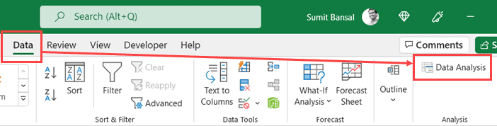
You can check whether you already have it enabled by going to the Data tab.
If you see the Data Analysis option in the Analysis group, you already have it enabled (and you can skip the next section and go directly to the ‘Getting Descriptive Analysis’ section).
In case you do not see the data analysis option in the data tab, follow the steps in the next section to enable it.
Enabling Data Analysis Toolpak
Below are the steps to enable the Data Analysis Toolpak in Excel:
- Open any Excel document
- Click the File tab

- Click on Options. This will open the Excel Options dialog box

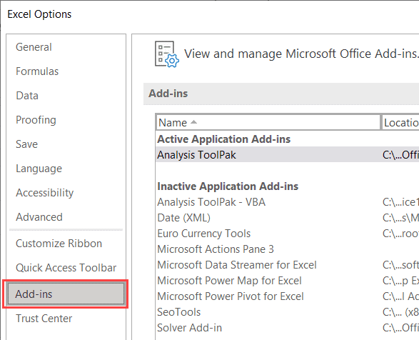
- In the Excel Options dialog box, click on Add-ins in the left pane
- From the Manage drop-down (which is at the bottom of the dialog box), select ‘Excel Add-ins’
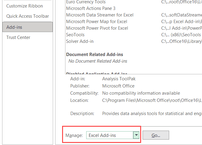
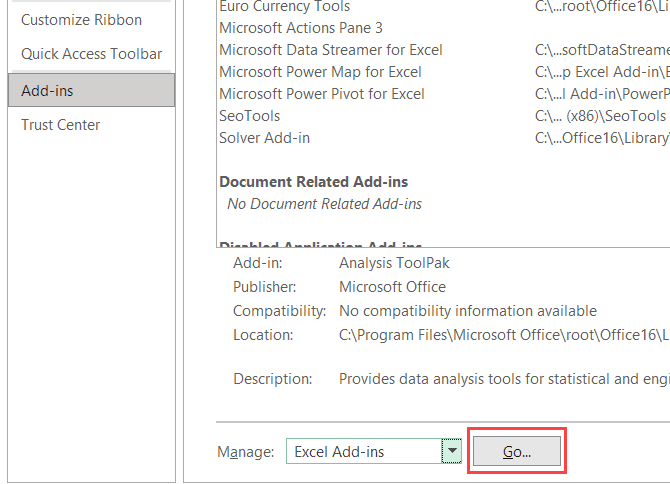
- Click on the Go button
- In the Add-ins dialog box that shows up, check the Analysis Toolpak option
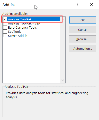
- Click OK
The other steps would enable the Data Analysis toolpak and you will be able to use it on all your Excel Workbooks.
Getting the Descriptive Analysis
Now that the Data Analysis Toolpak is enabled, let’s see how to get the descriptive statistics using it.
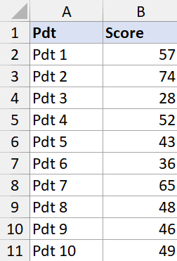
Suppose you have a data set as shown below where I have the sales data of different products of a company. For this data, I want to get descriptive statistics.
Below are the steps to do this:
- Click the Data tab
- In the Analysis group, click on Data Analysis
- In the Data Analysis dialog box that opens, click on Descriptive Statistics
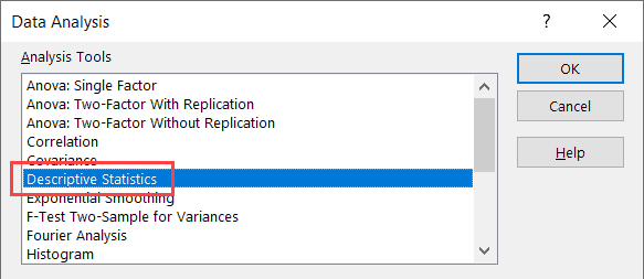
- Click OK
- In the Descriptive Statistics dialog box, specify the input range that has the data. Note that I have only used Column B as the data source (as you can only use numeric data as the input here)
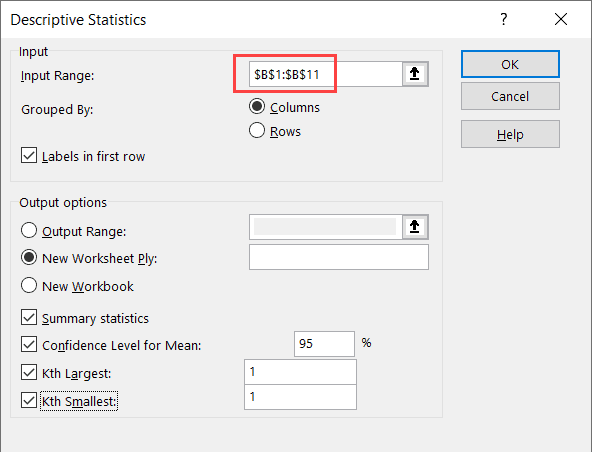
- If your data has headers, check the ‘Labels in first row’ option
- Select the New Worksheet Ply option (this will give the result in a new sheet)
- Select the statistics options you want (you need to select atleast one, and can select all four)
- Click OK
The above steps would insert a new sheet and you will get the statistics as shown below:
Note that you can specify the following in step 8:
- Confidence Level for mean – the default is 95%, but you can change the value
- Kth Largest – the default is 1, but you can change it. If you enter 3 here, it will give you the third largest value from the dataset
- Kth Smallest – the default is 1, but you can change it. If you enter 3 here, it will give you the third smallest value from the dataset
Note that the resulting values you get are static values.
In case your original data changes and you again want to get the Descriptive Statistics, you will have to repeat the above steps again.
So this is how you can quickly get Descriptive Statistics in Microsoft Excel.
I hope you found this tutorial useful.
Other Excel Tutorials you may also like:
- How to Calculate Standard Deviation in Excel
- How to Calculate PERCENTILE in Excel
- Calculating Weighted Average in Excel.
- Calculating CAGR in Excel
- How to Calculate Correlation Coefficient in Excel
- Calculate the Coefficient of Variation (CV) in Excel
To get detailed information about a function, click its name in the first column.
Note: Version markers indicate the version of Excel a function was introduced. These functions aren’t available in earlier versions. For example, a version marker of 2013 indicates that this function is available in Excel 2013 and all later versions.
|
Function |
Description |
|
AVEDEV function |
Returns the average of the absolute deviations of data points from their mean |
|
AVERAGE function |
Returns the average of its arguments |
|
AVERAGEA function |
Returns the average of its arguments, including numbers, text, and logical values |
|
AVERAGEIF function |
Returns the average (arithmetic mean) of all the cells in a range that meet a given criteria |
|
AVERAGEIFS function |
Returns the average (arithmetic mean) of all cells that meet multiple criteria |
|
BETA.DIST function |
Returns the beta cumulative distribution function |
|
BETA.INV function |
Returns the inverse of the cumulative distribution function for a specified beta distribution |
|
BINOM.DIST function |
Returns the individual term binomial distribution probability |
|
BINOM.DIST.RANGE function |
Returns the probability of a trial result using a binomial distribution |
|
BINOM.INV function |
Returns the smallest value for which the cumulative binomial distribution is less than or equal to a criterion value |
|
CHISQ.DIST function |
Returns the cumulative beta probability density function |
|
CHISQ.DIST.RT function |
Returns the one-tailed probability of the chi-squared distribution |
|
CHISQ.INV function |
Returns the cumulative beta probability density function |
|
CHISQ.INV.RT function |
Returns the inverse of the one-tailed probability of the chi-squared distribution |
|
CHISQ.TEST function |
Returns the test for independence |
|
CONFIDENCE.NORM function |
Returns the confidence interval for a population mean |
|
CONFIDENCE.T function |
Returns the confidence interval for a population mean, using a Student’s t distribution |
|
CORREL function |
Returns the correlation coefficient between two data sets |
|
COUNT function |
Counts how many numbers are in the list of arguments |
|
COUNTA function |
Counts how many values are in the list of arguments |
|
COUNTBLANK function |
Counts the number of blank cells within a range |
|
COUNTIF function |
Counts the number of cells within a range that meet the given criteria |
|
COUNTIFS function |
Counts the number of cells within a range that meet multiple criteria |
|
COVARIANCE.P function |
Returns covariance, the average of the products of paired deviations |
|
COVARIANCE.S function |
Returns the sample covariance, the average of the products deviations for each data point pair in two data sets |
|
DEVSQ function |
Returns the sum of squares of deviations |
|
EXPON.DIST function |
Returns the exponential distribution |
|
F.DIST function |
Returns the F probability distribution |
|
F.DIST.RT function |
Returns the F probability distribution |
|
F.INV function |
Returns the inverse of the F probability distribution |
|
F.INV.RT function |
Returns the inverse of the F probability distribution |
|
F.TEST function |
Returns the result of an F-test |
|
FISHER function |
Returns the Fisher transformation |
|
FISHERINV function |
Returns the inverse of the Fisher transformation |
|
FORECAST function |
Returns a value along a linear trend Note: In Excel 2016, this function is replaced with FORECAST.LINEAR as part of the new Forecasting functions, but it’s still available for compatibility with earlier versions. |
|
FORECAST.ETS function |
Returns a future value based on existing (historical) values by using the AAA version of the Exponential Smoothing (ETS) algorithm |
|
FORECAST.ETS.CONFINT function |
Returns a confidence interval for the forecast value at the specified target date |
|
FORECAST.ETS.SEASONALITY function |
Returns the length of the repetitive pattern Excel detects for the specified time series |
|
FORECAST.ETS.STAT function |
Returns a statistical value as a result of time series forecasting |
|
FORECAST.LINEAR function |
Returns a future value based on existing values |
|
FREQUENCY function |
Returns a frequency distribution as a vertical array |
|
GAMMA function |
Returns the gamma function value |
|
GAMMA.DIST function |
Returns the gamma distribution |
|
GAMMA.INV function |
Returns the inverse of the gamma cumulative distribution |
|
GAMMALN function |
Returns the natural logarithm of the gamma function, Γ(x) |
|
GAMMALN.PRECISE function |
Returns the natural logarithm of the gamma function, Γ(x) |
|
GAUSS function |
Returns 0.5 less than the standard normal cumulative distribution |
|
GEOMEAN function |
Returns the geometric mean |
|
GROWTH function |
Returns values along an exponential trend |
|
HARMEAN function |
Returns the harmonic mean |
|
HYPGEOM.DIST function |
Returns the hypergeometric distribution |
|
INTERCEPT function |
Returns the intercept of the linear regression line |
|
KURT function |
Returns the kurtosis of a data set |
|
LARGE function |
Returns the k-th largest value in a data set |
|
LINEST function |
Returns the parameters of a linear trend |
|
LOGEST function |
Returns the parameters of an exponential trend |
|
LOGNORM.DIST function |
Returns the cumulative lognormal distribution |
|
LOGNORM.INV function |
Returns the inverse of the lognormal cumulative distribution |
|
MAX function |
Returns the maximum value in a list of arguments |
|
MAXA function |
Returns the maximum value in a list of arguments, including numbers, text, and logical values |
|
MAXIFS function |
Returns the maximum value among cells specified by a given set of conditions or criteria |
|
MEDIAN function |
Returns the median of the given numbers |
|
MIN function |
Returns the minimum value in a list of arguments |
|
MINIFS function |
Returns the minimum value among cells specified by a given set of conditions or criteria. |
|
MINA function |
Returns the smallest value in a list of arguments, including numbers, text, and logical values |
|
MODE.MULT function |
Returns a vertical array of the most frequently occurring, or repetitive values in an array or range of data |
|
MODE.SNGL function |
Returns the most common value in a data set |
|
NEGBINOM.DIST function |
Returns the negative binomial distribution |
|
NORM.DIST function |
Returns the normal cumulative distribution |
|
NORM.INV function |
Returns the inverse of the normal cumulative distribution |
|
NORM.S.DIST function |
Returns the standard normal cumulative distribution |
|
NORM.S.INV function |
Returns the inverse of the standard normal cumulative distribution |
|
PEARSON function |
Returns the Pearson product moment correlation coefficient |
|
PERCENTILE.EXC function |
Returns the k-th percentile of values in a range, where k is in the range 0..1, exclusive. |
|
PERCENTILE.INC function |
Returns the k-th percentile of values in a range |
|
PERCENTRANK.EXC function |
Returns the rank of a value in a data set as a percentage (0..1, exclusive) of the data set |
|
PERCENTRANK.INC function |
Returns the percentage rank of a value in a data set |
|
PERMUT function |
Returns the number of permutations for a given number of objects |
|
PERMUTATIONA function |
Returns the number of permutations for a given number of objects (with repetitions) that can be selected from the total objects |
|
PHI function |
Returns the value of the density function for a standard normal distribution |
|
POISSON.DIST function |
Returns the Poisson distribution |
|
PROB function |
Returns the probability that values in a range are between two limits |
|
QUARTILE.EXC function |
Returns the quartile of the data set, based on percentile values from 0..1, exclusive |
|
QUARTILE.INC function |
Returns the quartile of a data set |
|
RANK.AVG function |
Returns the rank of a number in a list of numbers |
|
RANK.EQ function |
Returns the rank of a number in a list of numbers |
|
RSQ function |
Returns the square of the Pearson product moment correlation coefficient |
|
SKEW function |
Returns the skewness of a distribution |
|
SKEW.P function |
Returns the skewness of a distribution based on a population: a characterization of the degree of asymmetry of a distribution around its mean |
|
SLOPE function |
Returns the slope of the linear regression line |
|
SMALL function |
Returns the k-th smallest value in a data set |
|
STANDARDIZE function |
Returns a normalized value |
|
STDEV.P function |
Calculates standard deviation based on the entire population |
|
STDEV.S function |
Estimates standard deviation based on a sample |
|
STDEVA function |
Estimates standard deviation based on a sample, including numbers, text, and logical values |
|
STDEVPA function |
Calculates standard deviation based on the entire population, including numbers, text, and logical values |
|
STEYX function |
Returns the standard error of the predicted y-value for each x in the regression |
|
T.DIST function |
Returns the Percentage Points (probability) for the Student t-distribution |
|
T.DIST.2T function |
Returns the Percentage Points (probability) for the Student t-distribution |
|
T.DIST.RT function |
Returns the Student’s t-distribution |
|
T.INV function |
Returns the t-value of the Student’s t-distribution as a function of the probability and the degrees of freedom |
|
T.INV.2T function |
Returns the inverse of the Student’s t-distribution |
|
T.TEST function |
Returns the probability associated with a Student’s t-test |
|
TREND function |
Returns values along a linear trend |
|
TRIMMEAN function |
Returns the mean of the interior of a data set |
|
VAR.P function |
Calculates variance based on the entire population |
|
VAR.S function |
Estimates variance based on a sample |
|
VARA function |
Estimates variance based on a sample, including numbers, text, and logical values |
|
VARPA function |
Calculates variance based on the entire population, including numbers, text, and logical values |
|
WEIBULL.DIST function |
Returns the Weibull distribution |
|
Z.TEST function |
Returns the one-tailed probability-value of a z-test |


Important: The calculated results of formulas and some Excel worksheet functions may differ slightly between a Windows PC using x86 or x86-64 architecture and a Windows RT PC using ARM architecture. Learn more about the differences.
Related Topics
Excel functions (by category)
Excel functions (alphabetical)
To begin with, statistical function in Excel let’s first understand what is statistics and why we need it? So, statistics is a branch of sciences that can give a property to a sample. It deals with collecting, organizing, analyzing, and presenting the data. One of the great mathematicians Karl Pearson, also the father of modern statistics quoted that, “statistics is the grammar of science”.
We used statistics in every industry, including business, marketing, governance, engineering, health, etc. So in short statistics a quantitative tool to understand the world in a better way. For example, the government studies the demography of his/her country before making any policy and the demography can only study with the help of statistics. We can take another example for making a movie or any campaign it is very important to understand your audience and there too we used statistics as our tool.
Ways to approach statistical function in Excel:
In Excel, we have a range of statical functions, we can perform basic mead, median mode to more complex statistical distribution, and probability test. In order to understand statistical Functions we will divide them into two sets:
- Basic statistical Function
- Intermediate Statistical Function.
Statistical Function in Excel
Excel is the best tool to apply statistical functions. As discussed above we first discuss the basic statistical function, and then we will study intermediate statistical function. Throughout the article, we will take data and by using it we will understand the statistical function.
So, let’s take random data of a book store that sells textbooks for classes 11th and 12th.
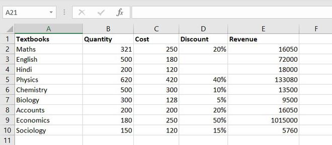
Example of statistical function.
Basic statistical Function
These are some most common and useful functions. These include the COUNT function, COUNTA function, COUNTBLANK function, COUNTIFS function. Let’s discuss one by one:
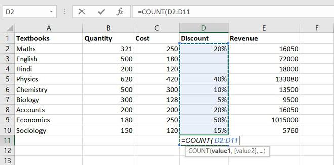
1. COUNT function
The COUNT function is used to count the number of cells containing a number. Always remember one thing that it will only count the number.
Formula for COUNT function = COUNT(value1, [value2], …)
Example of statistical function.
Thus, there are 7 textbooks that have a discount out of 9 books.
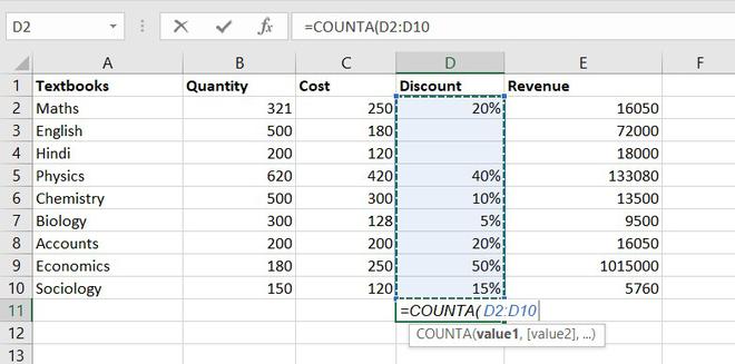
2. COUNTA function
This function will count everything, it will count the number of the cell containing any kind of information, including numbers, error values, empty text.
Formula for COUNTA function = COUNTA(value1, [value2], …)
Example of statistical function.
So, there are a total of 9 subjects that being sold in the store
3. COUNTBLANK function
COUNTBLANK function, as the term, suggest it will only count blank or empty cells.
Formula for COUNTBlANK function = COUNTBLANK(range)
![]()
Example of statistical function.
There are 2 subjects that don’t have any discount.
4. COUNTIFS function
COUNTIFS function is the most used function in Excel. The function will work on one or more than one condition in a given range and counts the cell that meets the condition.
Formula for COUNTIFS function = COUNTIFS (range1, criteria1, [range2], [criteria2], ...)
Intermediate Statistical Function
Let’s discuss some intermediate statistical functions in Excel. These functions used more often by the analyst. It includes functions like AVERAGE function, MEDIAN function, MODE function, STANDARD DEVIATION function, VARIANCE function, QUARTILES function, CORRELATION function.
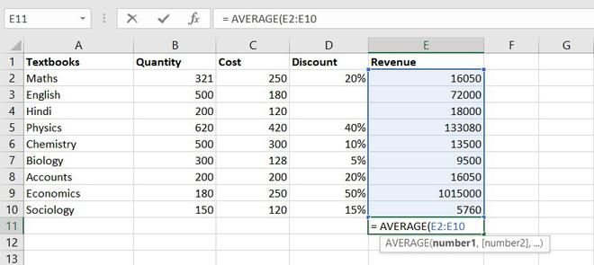
1. AVERAGE value1, [value2], …)
The AVERAGE function is one of the most used intermediate functions. The function will return the arithmetic mean or an average of the cell in a given range.
Formula for AVERAGE function = AVERAGE(number1, [number2], …)
Example of statistical function.
So the average total revenue is Rs.144326.6667
2. AVERAGEIF function
The function will return the arithmetic mean or an average of the cell in a given range that meets the given criteria.
Formula for AVERAGEIF function = AVERAGEIF(range, criteria, [average_range])
3. MEDIAN function
The MEDIAN function will return the central value of the data. Its syntax is similar to the AVERAGE function.
Formula for MEDIAN function = MEDIAN(number1, [number2], …)
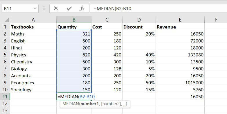
Example of statistical function.
Thus, the median quantity sold is 300.
4. MODE function
The MODE function will return the most frequent value of the cell in a given range.
Formula for MODE function = MODE.SNGL(number1,[number2],…)
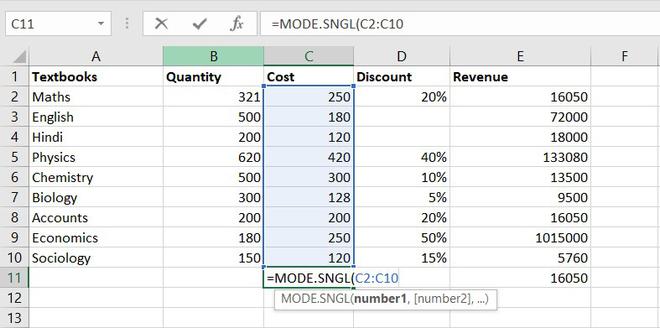
Example of statistical function.
Thus, the most frequent or repetitive cost is Rs. 250.
5. STANDARD DEVIATION
This function helps us to determine how much observed value deviated or varied from the average. This function is one of the useful functions in Excel.
Formula for STANDARD DEVIATION function = STDEV.P(number1,[number2],…)
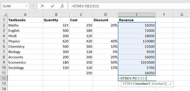
Example of statistical function.
Thus, Standard Deviation of total revenue =296917.8172
6. VARIANCE function
To understand the VARIANCE function, we first need to know what is variance? Basically, Variance will determine the degree of variation in your data set. The more data is spread it means the more is variance.
Formula for VARIANCE function = VAR(number1, [number2], …)
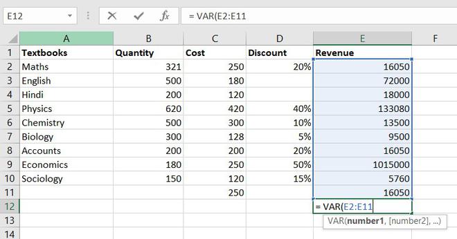
Example of statistical function.
So, the variance of Revenue= 97955766832
7. QUARTILES function
Quartile divides the data into 4 parts just like the median which divides the data into two equal parts. So, the Excel QUARTILES function returns the quartiles of the dataset. It can return the minimum value, first quartile, second quartile, third quartile, and max value. Let’s see the syntax :
Formula for QUARTILES function = QUARTILE (array, quart)
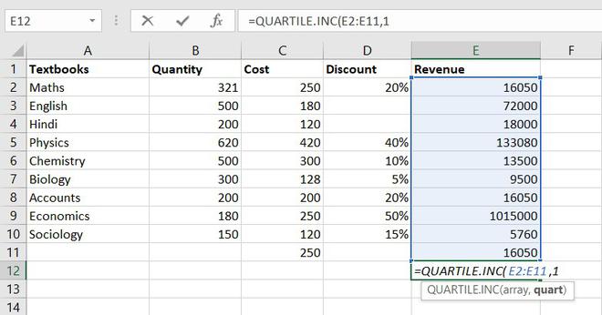
Example of statistical function.
So, the first quartile = 14137.5
8. CORRELATION function
CORRELATION function, help to find the relationship between the two variables, this function mostly used by the analyst to study the data. The range of the CORRELATION coefficient lies between -1 to +1.
Formula for CORRELATION function = CORREL(array1, array2)
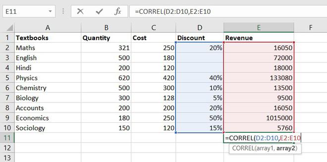
Example of statistical function.
So, the correlation coefficient between discount and revenue of store = 0.802428894. Since it is a positive number, thus we can conclude discount is positively related to revenue.
9. MAX function
The MAX function will return the largest numeric value within a given set of data or an array.
Formula for MAX function = MAX (number1, [number2], ...)
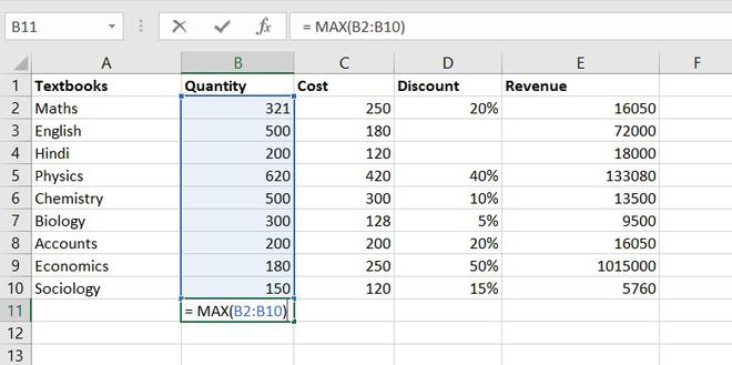
The maximum quantity of textbooks is Physics,620 in numbers.
10. MIN function
The MIN function will return the smallest numeric value within a given set of data or an array.
Formula for MIN function = MIN (number1, [number2], ...)
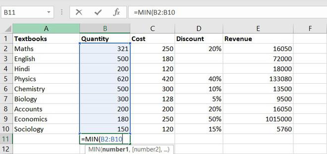
The minimum number of the book available in the store =150(Sociology)
11. LARGE function
The LARGE function is similar to the MAX function but the only difference is it returns the nth largest value within a given set of data or an array.
Formula for LARGE function = LARGE (array, k)
Let’s find the most expensive textbook using a large function, where k = 1
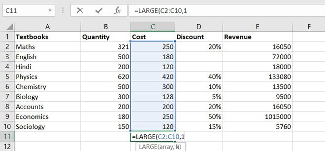
Example of statistical function.
The most expensive textbook is Rs. 420.
12. SMALL function
The SMALL function is similar to the MIN function, but the only difference is it return nth smallest value within a given set of data or an array.
Formula for SMALL function = SMALL (array, k)
Similarly, using the SMALL function we can find the second least expensive book.
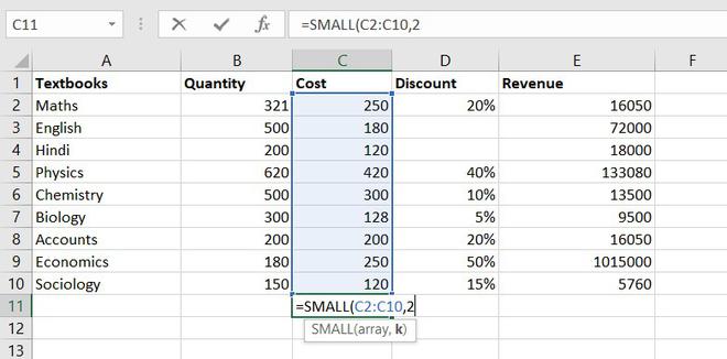
Example of statistical function.
Thus, Rs. 120 is the least cost price.
Conclusion
So these are some statistical functions of Excel. We have learned some of the most simple functions like COUNT functions to complex ones like the CORRELATION function. So far we learn, we understand how much these functions are useful for analyzing any data. You can explore more functions and learn more things of your own.
Microsoft Excel can do statistics! You can calculate percentages, averages, standard deviation, standard error, and student’s T-tests.

Despite not being as powerful as software specifically for statistics, Excel is actually quite adept at running basic calculations, even without add-ins (though there are some add-ins that make it even better).
You probably know that it can do arithmetic, but did you know that it can also quickly get percentage change, averages, standard deviation from samples and populations, standard error, and student’s T-tests?
Excel has a lot of statistical power if you know how to use it. We’ll take a look at some of the most basic statistical calculations below. Let’s get started!
How to Calculate Percentage in Excel
Calculating percentages in Excel is as simple as it is anywhere else: just divide two numbers and multiply by 100. Let’s say that we’re calculating the percentage of 347 out of 521.
Simply divide 347 by 521 using the syntax =347/521. (If you’re not familiar with Excel, the equals sign tells Excel that you want it to calculate something. Just enter the equation after that and hit Enter to run the calculation.)
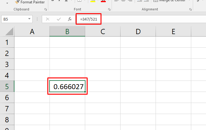
You now have a decimal value (in this case, .67). To convert it into a percentage, hit Ctrl + Shift + 5 on your keyboard (this is a very useful Excel keyboard shortcut to add to your arsenal).
You can also change the cell format the long way by right-clicking the cell, selecting Format Cells, choosing Percentage, and clicking OK.
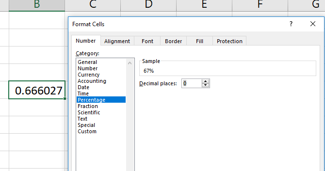
Keep in mind that changing the format of the cell takes care of the «multiply by 100» step. If you multiply by 100 and then change the format to percentage, you’ll get another multiplication (and the wrong number).
Tip: Learn how to create dropdown lists for Excel cells.
How to Calculate Percentage Increase in Excel
Calculating the percentage increase is similar. Let’s say our first measurement is 129, and our second is 246. What’s the percentage increase?
To start, you’ll need to find the raw increase, so subtract the initial value from the second value. In our case, we’ll use =246-129 to get a result of 117.
Now, take the resulting value (the raw change) and divide it by the original measurement. In our case, that’s =117/129. That gives us a decimal change of .906. You can also get all of this information in a single formula like this:
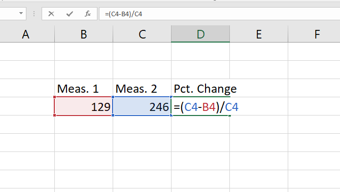
Use the same process as above to convert this to a percentage, and you’ll see that we have a 91 percent change. Do a quick check: 117 is almost equal to 129, so this makes sense. If we would have calculated a change value of 129, the percentage change would have been 100 percent.
How to Calculate Mean (Average) in Excel
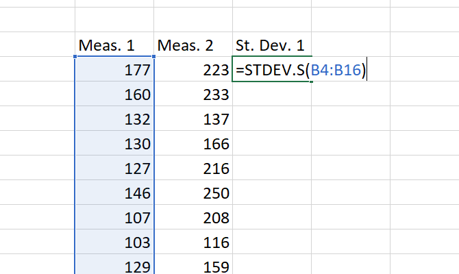
One of Excel’s most useful built-in functions calculates the mean (average) of a set of numbers. If you haven’t used an Excel function before, you’ll be impressed at how easy it is. Just type in the name of the function, select the cells you want to apply it to, and hit Enter.
In our example here, we have a series of measurements that we need the average of. We’ll click into a new cell and type =AVERAGE(, then use the mouse to select the relevant cells (you can also type in the cell range if you’d like). Close the parentheses with a ) and you’ll have a formula that looks like this: =AVERAGE(B4:B16)
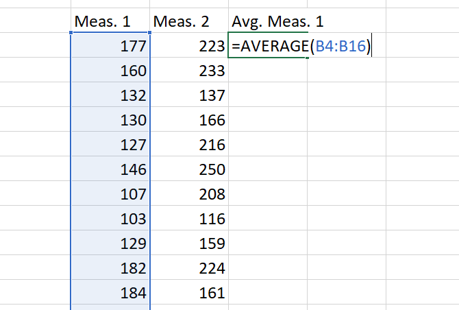
Hit Enter, and you’ll get the average! That’s all there is to it.
You can also use Excel to calculate the weighted average.
How to Calculate a Student’s T-Test in Excel
A Student’s t-test calculates the chances that two samples came from the same population. A lesson in statistics is beyond this article, but you can read up more on the different types of Student’s t-tests with these free resources for learning statistics (Statistics Hell is my personal favorite).
In short, though, the P-value derived from a Student’s t-test will tell you whether there’s a significant difference between two sets of numbers.
Let’s say you have two measurements from the same group and you want to see if they’re different. Say you weighed a group of participants, had them go through personal training, and then weighed them again. This is called a paired t-test, and we’ll start with this.
Excel’s T.TEST function is what you need here. The syntax looks like this:
=T.TEST(array1, array2, tails, type)
array1 and array2 are the groups of numbers you want to compare. The tails argument should be set to «1» for a one-tailed test and «2» for a two-tailed test.
The type argument can be set to «1,» «2,» or «3.» We’ll set it to «1» for this example because that’s how we tell Excel we’re doing a paired t-test.
Here’s what the formula will look like for our example:
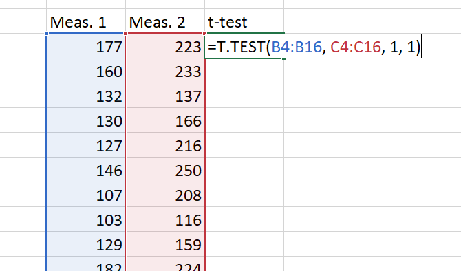
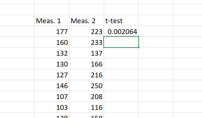
Now we just hit Enter to get our result! It’s important to remember that this result is the P value. In most fields, a P value of less than .05 indicates a significant result.
The basics of the test are the same for all three types. As mentioned, a «1» in the type field creates a paired t-test. A «2» runs a two-sample test with equal variance, and a «3» runs a two-sample test with unequal variance. (When using the latter, Excel runs a Welch’s t-test.)
How to Calculate Standard Deviation in Excel
Calculating standard deviation in Excel is just as easy as calculating the average. This time, you’ll use the STDEV.S or STDEV.P functions, though.
STDEV.S should be used when your data is a sample of a population. STDEV.P, on the other hand, works when you’re calculating the standard deviation for an entire population. Both of these functions ignore text and logical values (if you want to include those, you’ll need STDEVA or STDEVPA).
To determine the standard deviation for a set, just type =STDEV.S() or =STDEV.P() and insert the range of numbers into the parentheses. You can click-and-drag or type the range.
At the end, you’ll have a number: that’s your standard deviation.
How to Calculate Standard Error in Excel
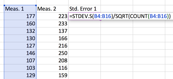
Standard error is closely related to standard deviation. And while Excel doesn’t have a function that will calculate it, you can quickly find it with minimal effort.
To find the standard error, divide the standard deviation by the square root of n, the number of values in your dataset. You can get this information with a single formula:
=STDEV.S(array1)/SQRT(COUNT(array1))
If you’re using text or logical values in your array, you’ll need to use COUNTA instead.
Here’s how we’d calculate the standard error with our dataset:
Using Excel for Statistics: Not Great but Workable
Can you use Excel for statistics and complex calculations? Yes. Will it work as well as dedicated statistical software like SPSS or SAS? No. But you can still calculate percentages, averages, standard deviations, and even t-tests.
When you need a quick calculation, and your data is in Excel, you don’t need to import it into different software. And that’ll save you time. You can also use Excel’s Goal Seek feature to solve equations even faster.
Don’t forget to put your data into aesthetically pleasing and informative graphs before you show it to your colleagues! And it would also help to master IF statements in Excel.
You can use the Analysis Toolpak add-in to generate descriptive statistics. For example, you may have the scores of 14 participants for a test.

To generate descriptive statistics for these scores, execute the following steps.
1. On the Data tab, in the Analysis group, click Data Analysis.

Note: can’t find the Data Analysis button? Click here to load the Analysis ToolPak add-in.
2. Select Descriptive Statistics and click OK.

3. Select the range A2:A15 as the Input Range.
4. Select cell C1 as the Output Range.
5. Make sure Summary statistics is checked.

6. Click OK.
Result:

Tip: visit our page about statistical functions to learn more about this topic.
In this tutorial, I will show you how to use the Data Analysis ToolPak to return some descriptive statistics about your data in Microsoft Excel. This includes the mean, standard error, median, mode and so much more.
How to install the Data Analysis ToolPak
A useful feature in Excel that many people do not know about is the Data Analysis ToolPak.
The Data Analysis ToolPak is an add-on created by Microsoft to make it easier to perform different data analysis procedures.
To ensure you have the Data Analysis ToolPak activated correctly, go to File>Options.
Then select Add-ins.
At the bottom, where it says Manage, ensure you select Excel Add-ins and click Go.
Ensure you have the Analysis ToolPak option ticked, and click the OK button.
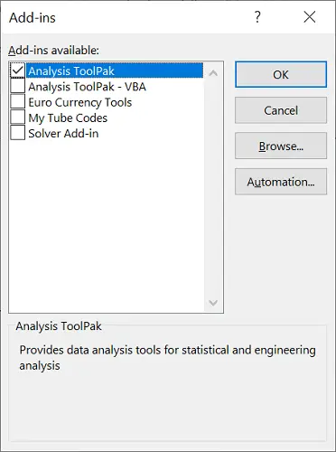
Now, when you select the Data tab at the top, you should see a Data Analysis button appears.
Now we’re ready to perform the descriptive statistics.
To perform descriptive statistics in Excel, go to Data>Data Analysis.
Then, from the list, select Descriptive Statistics.
This should open a new window.
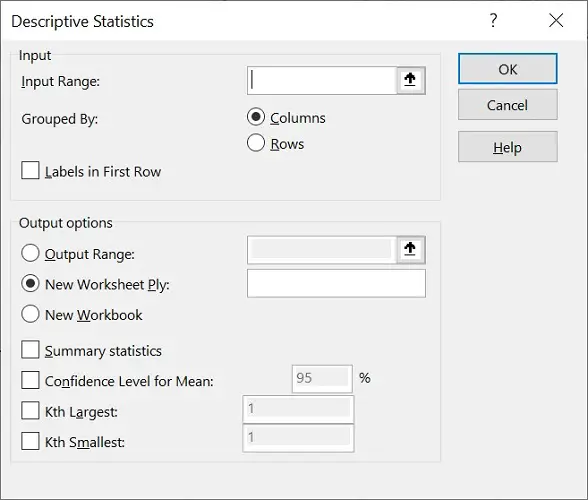
For the input range, this is where you enter the range of cells containing your data.
Next, need to tell Excel how your data are entered in your sheet.
If you have the values stacked in a column, then these will be grouped by columns. If they were entered into rows instead, then select the rows option.
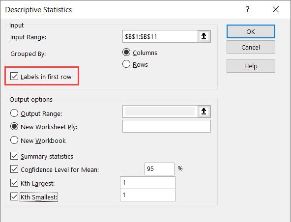
If you also have labels at the top of your data in the first row, then ensure you select Labels in First Row.
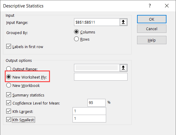
For the output options, this is where you specify where you want the descriptive statistics to be returned
There are three options:
- Output Range – Enter a specific cell in this same worksheet where you want the results to be entered
- New Worksheet Ply – Enter the results in a new worksheet
- New Workbook – Enter the descriptive statistics in an entirely new Excel file
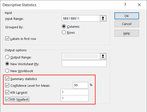
Underneath, you can tick the various descriptive statistic options that you want to perform. At a minimum, you will want to select the Summary Statistics. The Confidence Level for Mean, Kth Largest and Kth Smallest options are optional, and I will explain more about these later.
So that’s the setup done, now press the OK button to perform the descriptive statistics.
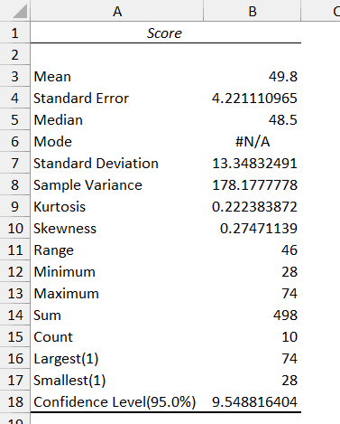
How to interpret the descriptive statistics results
Below are some descriptive statistics I have based on some example data. I’ll now go over and explain each output.
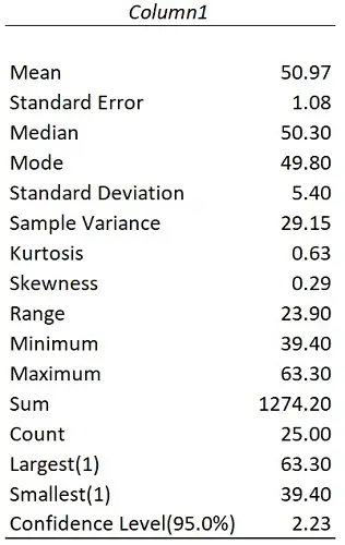
Mean
The first result is the mean, or average, value.
This is where you add all the values up in your sample and divide by the number of values in the sample.
To calculate the mean value youself, you can use the AVERAGE function.
=AVERAGE(data)
Standard error
The standard error is a measure of the variability of sample means in a sampling distribution of means.
The higher the standard error, the higher the variability.
You can calculate the standard error yourself by taking the standard deviation and dividing it by the square root of the count.
=STDEV.S(data)/SQRT(COUNT(data))
Median
Say we sorted our data in ascending order from smallest to largest. The median will be the number that lies in the middle of the values, in my case, the answer is 50.3.
You can calculate the median separately by using the MEDIAN function.
=MEDIAN(data)
Mode
The mode represents the value that appears the most in the sample
The mode for my example is 49.8 since this value appears twice.
If you want to calculate this yourself, you can use the MODE.SNGL function.
=MODE.SNGL(data)
Standard deviation
The standard deviation is a measure of the amount of variation in the data relative to the mean, where the higher the standard deviation, the higher the variability.
If you would like to calculate the standard deviation of a sample separately from the descriptive statistics, then use the STDEV.S function.
=STDEV.S(data)
Variance
The variance is simply the square of the standard deviation.
The Excel function for the variance of a sample is VAR.S.
=VAR.S(data)
Kurtosis
Kurtosis is a measure that defines how heavily the tails of a distribution differ from the tails of a normal distribution.
In Excel, a normal distribution has a kurtosis value of 0, positive values indicate a relatively peaked distribution and negative values indicate a relatively flat distribution.
You can use the KURT function to calculate the kurtosis separately.
=KURT(data)
Skewness
Skewness is a measure of asymmetry of the data distribution.
A value of 0 indicates a perfectly symmetrical distribution.
If the value is between -1 and 1, but isn’t 0, then the data are considered fairly skewed. If the value is outside this range, then the data are highly skewed.
The function for skewness is SKEW.
=SKEW(data)
Range
The range is simply the difference between the smallest and largest values in the data.
Minimum
The minimum is the smallest number in the data.
You can use the MIN function to work this out yourself.
=MIN(data)
Maximum
As the name suggests, the maximum is the largest number in the data.
To calculate this separately, use the MAX function.
=MAX(data)
SUM
The sum is the total calculated when you add up all the values in the data.
Use the SUM function to do this yourself.
=SUM(data)
Count
The count is the total number of values you have in your data.
Use the COUNT function to calculate the count separately.
=COUNT(data)
Kth largest
During the descriptive statistics setup, if you selected the Kth Largest option, then you’ll also have this result too.
Say you have 1 in the box next to the Kth Largest option, this would mean the first largest value in the data will be returned – in other words, the maximum.
If a 2 was used instead, then the second largest value will be returned, and so on and so forth.
Kth smallest
Similar to the above, if you selected the Kth Smallest option during the setup, then you’ll also have this result returned.
Having 1 entered during the setup will mean the first smallest value will be determined – the minimum value.
Again, changing this input to a 2 would mean the second smallest value is returned instead.
Confidence level
The last entry in the descriptive statistics table is the confidence interval value.
This is the value you can add and subtract from the mean to calculate the upper and lower confidence intervals, respectively. Specifically, these will be the 95% confidence intervals, since 95 was entered during the setup.
If you want to learn more about calculating confidence intervals in Microsoft Excel, then check out this post.
How to perform descriptive statistics in Excel: Final words
You should now know how to calculate some descriptive statistics in Excel.
Using the Data Analysis ToolPak makes this process so much easier and quicker than using separate functions.
Microsoft Excel version used: 365 ProPlus

Excel Statistics (Table of Contents)
- Introduction to Statistics in Excel
- Examples of Statistics in Excel
Introduction to Statistics in Excel
In this modern era where business solutions in a layman language are all people are thinking of, different dedicated software is developed and used for Statistical Analysis. It is a major part of the decision-making and finding out adequate solutions for your business problems. Despite the fact that it is not as powerful as the software designed dedicatedly for the Statistical Analysis, Excel still holds some of the power games to be able to do most of the Statistical Analytical tasks on its own and that too in a pretty simple manner. You need to be an advanced user of Excel, though, in order to be able to work on Statistical Analysis through Excel.
Examples of Statistics in Excel
We will see some examples using which we can calculate the statistics under Excel.
You can download this Statistics Excel Template here – Statistics Excel Template
Example #1 – Find Average
Suppose we have Country-wise Sales and Margin data as shown below:

We wanted to capture the average sales value for our company throughout these countries. The standard formula for Average is as below:
Average/Mean = Sum of All Values/ Number of Values
However, in Excel, you have a built-in AVERAGE function that does this task for you.
Step 1: In cell B9, start typing the formula =AVERAGE()

Step 2: Use B2:B7 (all sales values) as a reference under the AVERAGE function.

Step 3: Close the parentheses to complete the formula and press Enter key to see the output as shown below:

Step 4: Copy cell B9 and paste (Ctrl + V) it under cell C9 to get the average value for Margin. Well, this is one of the nicest Excel features of all time. You can copy the formulas and paste them to different cells so that you get the formulated results for the other column.

Example #2 – Margin Percentage for Each Country
Suppose we wanted to capture the Margin % we have acquired through business with each country. Does percentage show it all in a nice way, you know? Let’s see how this can be done.
The general formula for calculating Margin% is as follows:
Margin% = Margin/Sales
Step 1: In column D, under cell D2, use the formula as C2/B2 (Since C2 has Margin and B2 has Sales value for UAE).

Step 2: Press Enter key to see the Margin% value we have acquired for UAE through our trade.

Step 3: Now, Drag down this formula across the rows to see the Margin% we have acquired for different countries through trade. You can use the keyboard shortcut Ctrl + D to achieve the result. Select all the necessary sales, including D2 and press Ctrl + D.

We need to change the number formatting for column D to be seen in a percentage format. Follow the step below to achieve the result.
Step 4: Select entire column D. Go to Home tab, under which navigate towards Number group.

You can see the result as below:

Example #3 – Find Standard Deviation
We can also be very interested in knowing the degree to which the data points are deviating from our data. We can find out the Standard Deviation, which gives us a good idea about the spread of the data. It is very easy to calculate Standard Deviation under Excel. We have two functions to achieve the result.
STDEV.P and STDEV.S. STDEV.P works well when you have an entire population to cover, and STDEV.S is the one that can be used to figure out the Standard Deviation for a sample. Follow the steps below to be able to find the standard deviation.
Step 1: Start typing the formula under cell D10 as =STDEV.S( to initiate the formula for sample standard deviation.

Step 2: Now, use the range of cells you wanted to capture the standard deviation. I will use the sales values spread across B2:B7 as a reference to the STDEV.S function. It will give me a single value, which represents the standard deviation between the Sales Values.

Step 3: Use closing parentheses to complete the formula and press Enter key. You’ll get a Standard Deviation value as shown in the screenshot below:

Example #4 – Regression Analysis
Regression Analysis is a widely used statistical technique to determine a relationship between two or more variables and predict the future (forecasting) based on the model fitted. It assumes that there is some kind of relationship (termed as correlation) between two variables.
Suppose we have data of Height (in cm) and Weight (in kg) as shown below, and we are keen to know whether there is any relationship between both. If so, can we predict one based on the other?

This is a problem with Regression. Follow the steps below to run a regression analysis for the same.
Step 1: Navigate towards the Data tab and click on the Data Analysis button under the Analyze section.

Step 2: Once you click there, the Data Analysis toolbox will pop up. Scroll down to navigate towards and select Regression. Click OK.

Step 3: Use B2:B11 as Input Y Range and A2:A11 as Input X Range under the Regression window that pops up.

Step 4: Tick the Labels option, select Output Range as E2 of the current worksheet, and tick on Residuals to show the residuals for the data.

Step 5: Click the OK button once you are satisfied with the output options you chose. It is customizable; feel free to add some more residuals if you want.

You can see a regression output as shown in the image below under the same worksheet where data is present.

This is how we can use the statistical techniques in Excel to extract more analytical insights through our data. This article ends here.
Things to Remember
- There are more Statistical functions than the ones we have used in this article. Most of the formulae could be found under More Functions > Statistical functions encapsulated under Formulas sections.
- All basic Descriptive Statistics can also be calculated at once using Data Analysis Descriptive Statistics tool. This will capture Mean, Mode, Median, Range, Quartiles, Quartile Deviations, etc., for you at a single click.
- Working with advanced statistical techniques such as Regression, ANOVA, T-Test, F-Test, etc., is really very easy within Excel. I mean, come on! All you need to do is select an appropriate technique and do some clicking.’
Recommended Articles
This has been a guide to Statistics in Excel. Here we discuss How to use Statistics in Excel along with practical examples and a downloadable excel template. You can also go through our other suggested articles –
- Linear Interpolation in Excel
- Excel Regression Analysis
- Regression Line Formula
- Excel GROWTH Formula