
Excel for Microsoft 365 Excel for Microsoft 365 for Mac Excel for the web Excel 2021 Excel 2021 for Mac Excel 2019 Excel 2019 for Mac Excel 2016 Excel 2016 for Mac Excel 2013 Excel 2010 Excel 2007 Excel for Mac 2011 More…Less
Sometimes percentages can be frustrating because it’s not always easy to remember what we learned about them in school. Let Excel do the work for you – simple formulas can help you find the percentage of a total, for example, or the percentage difference between two numbers.
Find the percentage of a total
Let’s say that you answered 42 questions out of 50 correctly on a test. What is the percentage of correct answers?
-
Click any blank cell.
-
Type =42/50, and then press RETURN .
The result is 0.84.
-
Select the cell that contains the result from step 2.
-
On the Home tab, click
 .
.The result is 84.00%, which is the percentage of correct answers on the test.
Note: To change the number of decimal places that appear in the result, click Increase Decimal
or Decrease Decimal .
Find the percentage of change between two numbers
Let’s say that your earnings are $2,342 in November and $2,500 in December. What is the percentage of change in your earnings between these two months? Then, if your earnings are $2,425 in January, what is the percentage of change in your earnings between December and January? You can calculate the difference by subtracting your new earnings from your original earnings, and then dividing the result by your original earnings.
Calculate a percentage of increase
-
Click any blank cell.
-
Type =(2500-2342)/2342, and then press RETURN .
The result is 0.06746.
-
Select the cell that contains the result from step 2.
-
On the Home tab, click
.The result is 6.75%, which is the percentage of increase in earnings.
Note: To change the number of decimal places that appear in the result, click Increase Decimal
or Decrease Decimal .
Calculate a percentage of decrease
-
Click any blank cell.
-
Type =(2425-2500)/2500, and then press RETURN .
The result is -0.03000.
-
Select the cell that contains the result from step 2.
-
On the Home tab, click
.The result is -3.00%, which is the percentage of decrease in earnings.
Note: To change the number of decimal places that appear in the result, click Increase Decimal
or Decrease Decimal .
Find the total when you know the amount and percentage
Let’s say that the sale price of a shirt is $15, which is 25% off the original price. What is the original price? In this example, you want to find 75% of which number equals 15.
-
Click any blank cell.
-
Type =15/0.75, and then press RETURN .
The result is 20.
-
Select the cell that contains the result from step 2.
-
In newer versions:
On the Home tab, click
.The result is $20.00, which is the original price of the shirt.
In Excel for Mac 2011:
On the Home tab, under Number, click Currency
The result is $20.00, which is the original price of the shirt.
Note: To change the number of decimal places that appear in the result, click Increase Decimal
or Decrease Decimal .
Find an amount when you know the total and percentage
Let’s say that want to purchase a computer for $800 and must pay an additional 8.9% in sales tax. How much do you have to pay for the sales tax? In this example, you want to find 8.9% of 800.
-
Click any blank cell.
-
Type =800*0.089, and then press RETURN.
The result is 71.2.
-
Select the cell that contains the result from step 2.
-
In newer versions:
On the Home tab, click
.In Excel for Mac 2011:
On the Home tab, under Number, click Currency
The result is $71.20, which is the sales tax amount for the computer.
Note: To change the number of decimal places that appear in the result, click Increase Decimal
or Decrease Decimal .
Increase or decrease a number by a percentage
Let’s say that you spend an average of $113 on food each week, and you want to increase your weekly food expenditures by 25%. How much can you spend? Or, if you want to decrease your weekly food allowance of $113 by 25%, what is your new weekly allowance?
Increase a number by a percentage
-
Click any blank cell.
-
Type =113*(1+0.25), and then press RETURN .
The result is 141.25.
-
Select the cell that contains the result from step 2.
-
In newer versions:
On the Home tab, click
.In Excel for Mac 2011:
On the Home tab, under Number, click Currency
The result is $141.25, which is a 25% increase in weekly food expenditures.
Note: To change the number of decimal places that appear in the result, click Increase Decimal
or Decrease Decimal .
Decrease a number by a percentage
-
Click any blank cell.
-
Type =113*(1-0.25), and then press RETURN .
The result is 84.75.
-
Select the cell that contains the result from step 2.
-
In newer versions:
On the Home tab, click
.In Excel for Mac 2011:
On the Home tab, under Number, click Currency
The result is $84.75, which is a 25% reduction in weekly food expenditures.
Note: To change the number of decimal places that appear in the result, click Increase Decimal
or Decrease Decimal .
See also
PERCENTRANK function
Calculate a running total
Calculate an average
Need more help?
Want more options?
Explore subscription benefits, browse training courses, learn how to secure your device, and more.
Communities help you ask and answer questions, give feedback, and hear from experts with rich knowledge.
In various activities it is necessary to calculate percentages. We should understand, how do we «get» them. Trade allowances, VAT, discounts, profitability of deposits, securities and even tips — all these are calculated in the form of some part from the whole.
Let’s figure out how to work with the percentages in Excel. This program calculates automatically and admits different variants of the same formula.
Working with percentages in Excel
To count the percentage of the number, add, and take percentages on a modern calculator is not difficult. The main condition is the corresponding icon (%) on the keyboard. And only then it’s the matter of technology and mindfulness.
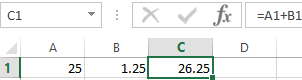
For example 25 + 5%. To find the value of the expression, you need to type on the calculator a given sequence of numbers and signs. The result is 26.25. With such a technique the great intellect is not needed.
To formulate formulas in Excel, let us recollect the school basics:
Percentage is one hundredth part of the whole.
To find a percentage of an integer, we should divide the required fraction by an integer and multiply by 100.
Example: 30 pieces of goods were bought. On the first day 5 units were sold. How many percentages of goods were sold?
5 is a part. 30 is an integer. We substitute data into the formula:
(5/30) * 100 = 16.7%
To add a percentage to a number in Excel (25 + 5%), you must first find 5% of 25. At school there was the proportion:
- 25 — 100%;
- Х — 5%.
X = (25 * 5) / 100 = 1.25
After that you can perform the addition. When the basic computing skills are restored, it is easy to understand the formulas.
How to calculate the percentage from the number in Excel
There are several ways.
Adapt the mathematical formula to the program: (Part / Whole) * 100.
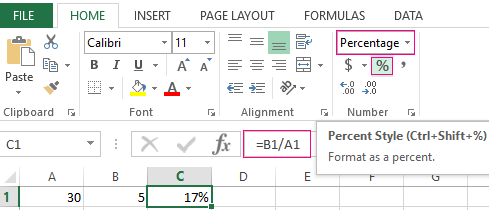
Look attentively at the formula line and the result. The result turned out to be correct. But we did not multiply by 100. Why?
In Excel the format of the cells changes. For C1, we have assigned a «Percentage» format. It means multiplying the value by 100 and putting it on the screen with the sign %. If necessary, you can set a certain number of digits after the decimal point.
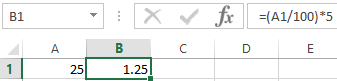
Now let’s calculate how much will be 5% of 25. To do this, enter the formula in the cell: = (25 * 5) / 100. The result is:
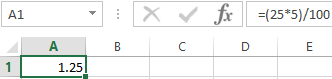
Another variant is = (25/100) * 5. The result will be the same.
Let’s have the example in another way by using the % sign on the keyboard:
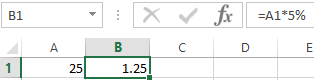
Let us apply this knowledge to practice.
The cost of the goods and the VAT rate (18%) are known. We need to calculate the amount of VAT.
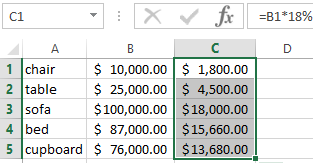
We multiply the cost of goods by 18%. Copy the formula for the whole column. To do this, we catch the mouse with the lower right corner of the cell and pull it down.
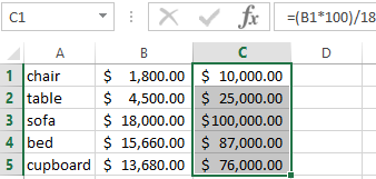
The amount of VAT, the rate is known. We should find the value of the goods. Calculation formula is: = (B1 * 100) / 18. The result is:
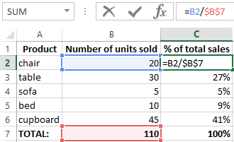
The quantity of the sold goods is known, separately and the whole. It is necessary to find the share of sales for each unit relative to the whole. The calculation formula remains the same: Part / Whole * 100. Only in this example we make the reference to the cell in the denominator of the fraction absolute. Use the $ sign in front of the line name and column name: $B$7.
How to add the percent to number
The task is solved in two actions:
- Firstly, we find how much a percentage of the number is. Here we calculated how much will be 5% of 25.
- Secondly, we add the result to the number. Example for review: 25 + 5%.
And here we performed the actual addition. Omit the intermediate effect.
The VAT rate is 18%. We need to find the amount of VAT and add it to the price of the goods. The formula is: =price + (price * 18%).
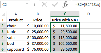
Do not forget about the brackets! With the help of it we establish the calculation procedure.
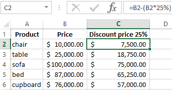
To remove the percentage from a number in Excel, you should follow the same procedure. We perform subtraction instead of addition.
How to count the odds in percentage in Excel?
What is the amount of the value changing between the two values in percentage?
First, let’s abstract from Excel. A month ago, the tables were brought to the store at a price of 100$ per unit. Today, the purchase price is 150$.
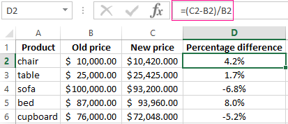
Difference in percentage is: = (New price – Old price) / Old price * 100%.
In our example, the purchase price for a unit of goods increased in 50%.
Let’s calculate the percentage difference between the data in two columns:
Do not forget to expose the «Percentage» format of the cells. Calculate the percentage difference between the lines:
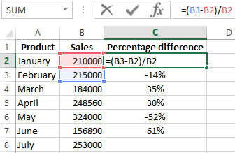
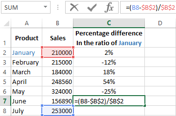
The formula is as follows: =(next value – previous value) / previous value.
With such an arrangement of the data, the first line is skipped!
If you want to compare the data for all months with January, for example, use the absolute reference to the cell with the desired value ($ sign).
How to make a diagram with percentages
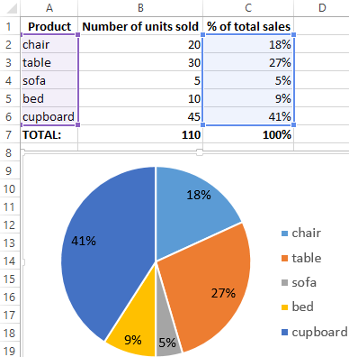
The first option is to make a column in the data table. Select 2 cell ranges A2:A6 and C2:C6 (while holding down the CTRL key). Then use this data to build a chart. Select the cells with percentages and copy — click «INSERT» — select the type of chart (for example «2D Pie») — OK.
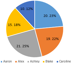
The second option: specify the format of data signatures in the form of a share. There are 22 working shifts in May. You need to calculate the percentage: the amount of work each worker did. We compose the table, where the first column is the number of working days; the second is the number of days off.
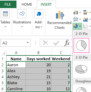
We make a pie chart. Select the data in cell ranges A2:C6. «INSERT» — «Insert Pie or Doughnut Chart» — «2D Pie».
Click on them with the right mouse button — «Add Data Labels» and «Format Data Labels»:
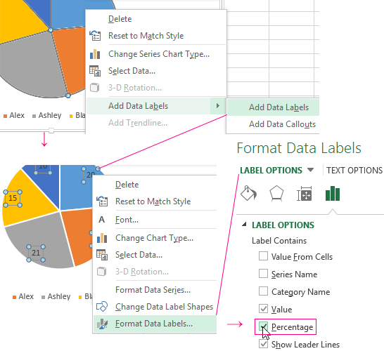
Choose «Share». On the tab «LABEL OPTIONS» we choose the percentage format. It turns out like this:
Download examples Calculate Percentages in Excel
We may stop here. And you can edit it to your taste: change the color, the appearance of the diagram, makes underscores and so on.
If you need to work with percentages, you’ll be happy to know that Excel has tools to make your life easier.
You can use Excel to calculate percentage increases or decreases to track your business results each month. Whether it’s rising costs or percentage sales changes from month to month, you want to keep on top of your key business figures. Excel can help you do that.
You’ll also learn how to work with advanced percentage calculations using the scenario of calculating grade point averages, as well as discover how to figure out percentile rankings, which are both relatable examples that you can apply to a variety of use cases.
In this tutorial, learn how to calculate percentages in Excel with step-by-step workflows. Let’s look at some Excel percentage formulas, functions, and tips using a sheet of business expenses and a sheet of school grades.
You’ll walk away with the techniques needed to work proficiently with percentages in Excel.
Screencast
Watch the complete tutorial screencast, or work through the step-by-step written version below. First, download the source files for free: Excel percentages worksheets. We’ll use them to work through the tutorial exercises.
1. Input
Initial Data in Excel
Input the data as follows (or start with the download file
«percentages.xlsx» contained in the tutorial source files). This worksheet is for Expenses. Later in this tutorial, we’ll
use the Grades worksheet.


2. Calculate a Percentage Increase
Let’s say you anticipate that next year’s costs will be 8%
higher, so you want to see what they are.
Before writing any formulas, it’s helpful to know that Excel
is flexible enough to calculate the same way whether you type percentages with
a percent sign (like 20%) or as a decimal (like 0.2 or just .2). To Excel, the
percent symbol is just formatting.
We want to show the total estimated amount, not just the increase.
Step 1
In A18, type the
header With 8% increase. Since we
have a number mixed with text, Excel will treat the entire cell as text.
Step 2
Press Tab, then
in B18, enter this Excel percentage formula: =B17 * 1.08
Alternatively, you can enter the formula this way: =B17 * 108%
The amount is 71,675, as shown below:


3. Calculate a Percentage Decrease
Maybe you think your expenses will decrease by 8 percent
instead. To see those numbers, the formula is similar. Start by showing the
total, lower amount, not just the decrease.
Step 1
In A19, type the
header With 8% decrease.
Step 2
Press Tab, then
in B19, enter this percentage formula in Excel: =B17 * .92
Alternatively, you can enter the formula this way: =B17 * 92%
The amount is 61,057.


Step 3
If you want a little more flexibility in changing the
percentage by which you think the costs will rise or drop, you can enter the
formulas this way, instead:
For the 8% increase, enter this formula in B18: =B17 + B17 * 0.08
Step 4
For the 8% decrease, enter this Excel percentage formula in B19: =B17 – B17 * 0.08
With these formulas, you can simply change the .08 to
another number to get a new result from a different percentage.
4. Calculate a Percentage Amount
Now to work through an Excel formula for a percentage amount. What if you want to see the 8% amount itself, not the new total? To do that, multiply the total
amount in B17 by 8 percent.
Step 1
In A20, enter the header 8% of total.
Step 2
Press Tab, then
in B20 enter the formula: =B17 * 0.08
Alternatively, you can enter the formula this way: =B17 * 8%
The amount is 5,309.


5. Make Adjustments Without Rewriting Formulas
If you want to change the percentage without having to
rewrite the formulas, put the percentage in its own cell. We’ll start by
entering row titles.
Step 1
In A22, type Adjustment.
Press Enter.
Step 2
In A23, type Higher
total. Press Enter.
Step 3
In A24, type Lower
total. Press Enter.
The worksheet should now look like this:


Now enter the percentage and the formulas to the right of
the titles.
Step 4
In B22, type 8%. Press Enter.
Step 5
In B23, enter
this formula to give you the total plus another 8%: =B17 + B17 * B22
Step 6
In B24, enter this
formula to give you the total less 8%: =B17 * (100% - B22)
When you type the 8% in B22, Excel automatically formats the
cell as a percentage. If you type .08 or 0.08, Excel will leave it like that.
You can always format it as a percent later on by clicking the Percent Style
button on the Ribbon:


Tip: you can also format the numbers as Percent Style using
a keyboard shortcut: press Control—Shift—% in Windows or Command-Shift-% on the Mac.
6. Calculate a Percentage Change
You might also want to calculate the percentage change from
one month to the next month. That would give you a picture of whether costs
were heading up or heading down. So let’s do that down column C.
The general rule to calculate a percentage change is:
=(new value — old
value) / new value
Since January is the first month, it doesn’t have a
percentage change. The first change will be from January to February, and we’ll
put this next to February’s number.
Step 1
To calculate the first percentage change, enter this percent change formula in C5: =(B5-B4)/B5
Step 2
Excel displays this as a decimal, so click the Percent Style
button on the Ribbon (or use the above mentioned shortcuts) to format it as a
percent.


Now that we know what the percent change is from January to
February, we can AutoFill the formula down column C to show the remaining percent
changes for the year.
Step 3
Roll the mouse pointer over the dot in the lower-right
corner of the cell that shows -7%.


Step 4
When the mouse pointer becomes a crosshair, Double-click.
If you’re unfamiliar with the AutoFill feature, see technique 3 in my Excel power techniques article:
Step 5
Click cell B3
(the “Amount” header).
Step 6
Put the mouse pointer on its AutoFill dot and drag one cell to
the right, into C3. That duplicates the
header, including the formatting.
Step 7
In C3, type % Change, replacing the text that’s already
there.


7. Calculate a Percentage of Total
The final technique on this sheet is to find the percent of
total for each month. For a percent of total calculation, think of a pie chart
where each month is a slice, and all the slices add up to 100%.
Whether with Excel or with pencil and paper, the way to
calculate a percentage of total is with a simple division:
Component
number/total
… and format it as a percentage.
In this example, we divide each month by the total at the
bottom of column B.
Step 1
Click on C3 and
AutoFill one cell across to D3.
Step 2
Change D3 to % of Total.
Step 3
In D4, type this
formula, but don’t press Enter, yet: =B4/B17
Step 4
Before entering the formula, we want to be sure of preventing
AutoFill errors. Since we’re going to AutoFill down the column, the denominator,
which is now B17, shouldn’t change. If it does, the numbers for February
through December will be wrong.
Make sure the text cursor is still in the formula, on the “B17”
denominator.
Step 5
Press the F4 key
(on the Mac, press Fn—F4).
That inserts dollar signs before the column and the row, turning
the denominator into $B$17. The $B means that column B won’t increase to column
C, etc. and the $17 means the row won’t increase to $18, etc.
Step 6
Make sure the percentage formula in excel is now: =B4/$B$17.


Step 7
Now we can enter and AutoFill.
Press Control-Enter (on the Mac, press Command-↩)
to enter the formula without moving the cursor down to the next row.
Step 8
Click the Percent
Style button on the ribbon or use the Control-Shift-% (Command-Shift-%) shortcut.
Step 9
Roll the mouse pointer over the AutoFill dot in the
lower-right corner of D4.
Step 10
When the cursor becomes a crosshair, double-click to
AutoFill the formula down to the bottom.
Each month will now show how much of a percentage of the
grand total it is.


8. Percentage Ranking
Ranking numbers by percent is a statistical technique.
You’re probably familiar with it from school: you and your classmates have
grade point averages, so each of you is ranked in a percentile. The higher your
grades, the higher your percentile.
The list of numbers (grades, in this
example) are in a range of cells that Excel calls an array. There’s nothing
special about an array and you don’t have to define it. That’s just what Excel
calls the range of cells you plug into a formula.
Excel has two functions for percentage ranking. One function
includes the beginning and ending numbers of the array and the other function
doesn’t.
Look at the second tab in the worksheet: Grades.


This shows a list of 35 grade point averages, sorted in
ascending order. The first thing we want to do is find the percentile rank for
each one. To do this, we’ll use the =PERCENTRANK.INC function. The “INC” part
of that function means “inclusive,» as it will include the first and last grades
in the list. If you want to exclude the first and last numbers in the array,
you would use the =PERCENTRANK.EXC function.
The function takes two mandatory arguments and the syntax
is: =PERCENTRANK.INC(array,
entry)
-
array is the
range of cells that contains the list (in this example, it’s B3:B37) -
entry is any
number or cell in the list
Step 1
Click C3, the
first one in the list.
Step 2
Start typing this formula, but don’t press Enter, yet: =PERCENTRANK.INC(B3:B37
Step 3
This range needs to be an absolute reference so we can
AutoFill to the bottom.
Press F4 (on the
Mac, press Fn—F4) to insert dollar signs.
The formula should now look like this: =PERCENTRANK.INC($B$3:$B$37
Step 4
In each case down column C, we want to know the percent rank
of the entry in column B.
Click B3, then
close the parenthesis.
The formula is now
this: =PERCENTRANK.INC($B$3:$B$37,B3)


Now we can fill in and format the numbers.
Step 5
If necessary, click back on C3 to select it.
Step 6
Double-click the AutoFill dot on C3. That automatically fills down the column.
Step 7
On the Ribbon, click the Percent Style button to format the
column as percentages. You should now see the finished result:
![]()
![]()
![]()
So if you had very good grades and your GPA was 3.98, you
would say that you ranked in the 94th percentile.
9. Finding the Percentile
You can also find the percentile directly, using the PERCENTILE
functions. With these functions, you enter a percent rank, and it will return a
number from the array that corresponds to that rank. If the exact number you
want isn’t listed, Excel will interpolate the result and return the number that
“should” be there.
When would you use this? Let’s say you plan on applying for
a graduate program, and the program accepts only students who score in the 60th percentile or higher. So you want to know what GPA is exactly 60%. Looking at
this list, we can see 3.22 is at 59% and 3.25 is at 62%, so we can use the
=PERCENTILE.INC function to find the answer.
The syntax is: =PERCENTILE.INC(array,
percent rank)
-
array is the
range of cells that contains the list (same as the previous example, B3:B37) -
rank is a
percentage (or a decimal between and including 0 and 1)
Just like with the percent ranking functions, you could use =PERCENTILE.EXC
to exclude the first and last entries in the array, but that’s not what we want
in this example.
Step 1
Click in B39,
below the list.
Step 2
Enter this formula: =PERCENTILE.INC(B3:B37,60%)
Since we aren’t going to AutoFill this formula, there is no
need to make the array an absolute reference.
Step 3
On the Ribbon, click the Decrease Decimal button once, to round the number to two decimal
places.
The result is that in this array, a 3.23 GPA is the 60th percentile. Now you know the grades you need for acceptance into the program.


Conclusion
Percentages aren’t complicated, and Excel calculates them
using the same rules of math as you would use with pencil and paper. Excel also
adheres to the standard order of operations when you have addition, subtraction, and multiplication in a formula:
- Parentheses
- Exponents
- Multiplication
- Division
- Addition
- Subtraction
I always remember this with the mnemonic Please Excuse My Dear Aunt Sally.
Did you find this post useful?

Bob Flisser has authored many videos and books about Microsoft and Adobe products, and has been a computer trainer since the 1980s. He is also a web and multimedia developer. Bob is a graduate of The George Washington University with a degree in financial economics.
Содержание
- Format numbers as percentages
- In this article
- How Excel handles percentages
- Display numbers as percentages
- Tips for displaying percentages
- Examples of calculating percentages
- Example 1: Increase or decrease a number by a percentage
- Example 2: Calculate an amount based on a percentage
- Example 3: Calculate the percentage based on two amounts
- Example 4: Calculate an amount based another amount and a percentage
- Example 5: Calculate the difference between two numbers and show it as a percentage
- Need more help?
- Calculate percentages
- Find the percentage of a total
- Find the percentage of change between two numbers
- Find the total when you know the amount and percentage
- Find an amount when you know the total and percentage
- Increase or decrease a number by a percentage
Format numbers as percentages
Learn how to display numbers as percentages in Excel and view examples of several basic techniques for calculating percentages in your worksheet.
In this article
How Excel handles percentages
Although formatting numbers as percentages is straightforward, the results you get after you apply the format may vary, depending on whether the numbers already exist in your workbook.
Formatting cells that already contain numbers If you apply the Percentage format to existing numbers in a workbook, Excel multiplies those numbers by 100 to convert them to percentages. For example, if a cell contains the number 10, Excel multiplies that number by 100, which means that you will see 1000.00% after you apply the Percentage format. This may not be what you expected. To accurately display percentages, before you format the numbers as a percentage, make sure that they have been calculated as percentages, and that they are displayed in decimal format. Percentages are calculated by using the equation amount / total = percentage. For example, if a cell contains the formula =10/100, the result of that calculation is 0.1. If you then format 0.1 as a percentage, the number will be correctly displayed as 10%. To learn more about calculating percentages, see Examples of calculating percentages.
Formatting empty cells If you apply the Percentage format to cells, and then type numbers into those cells, the behavior is different. Numbers equal to and larger than 1 are converted to percentages by default; and numbers smaller than 1 are multiplied by 100 to convert them to percentages. For example, typing 10 or 0.1 both result in 10.00%. (If you don’t want to display the two zeros after the decimal point, it’s easy to get rid of them, as explained in the following procedure.)
Display numbers as percentages
To quickly apply percentage formatting to selected cells, click Percent Style  in the Number group on the Home tab, or press Ctrl+Shift+%. If you want more control over the format, or you want to change other aspects of formatting for your selection, you can follow these steps.
On the Home tab, in the Number group, click the icon next to Number to display the Format Cells dialog box.

In the Format Cells dialog box, in the Category list, click Percentage.
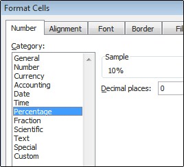
In the Decimal places box, enter the number of decimal places that you want to display. For example, if you want to see 10% instead of 10.00%, enter 0 in the Decimal places box.
Tips for displaying percentages
To reset the number format of selected cells, click General in the Category list. Cells that are formatted with the General format have no specific number format.
If you want negative percentages to stand out—for example, you want them to appear in red—you can create a custom number format ( Format Cells dialog box, Number tab, Custom category). The format should resemble the following: 0.00%;[Red]-0.00%. When applied to cells, this format displays positive percentages in the default text color and negative percentages in red. The portion that follows the semicolon represents the format that is applied to a negative value.

Similarly, you can display negative percentages in parentheses by creating a custom format that resembles this one: 0.00%_);(0.00%). For more information about how to create custom formats, see Create or delete a custom number format.
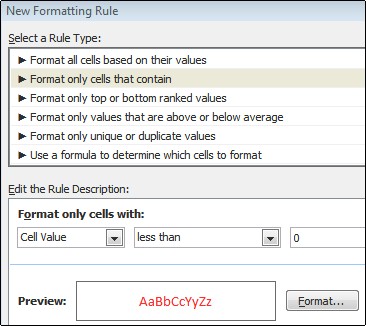
You can also use conditional formatting ( Home tab, Styles group, Conditional Formatting) to customize the way negative percentages appear in your workbook. The conditional formatting rule you create should be similar to the one shown in the following example. This particular rule instructs Excel to apply a format (red text) to a cell if the cell value is less than zero. For more information about conditional formatting, see Add, change, find, or clear conditional formats.
Examples of calculating percentages
This section shows several simple techniques for calculating percentages.
Example 1: Increase or decrease a number by a percentage
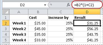
Scenario If you spend an average of $25 on food each week, and you want to cut your weekly food expenditures by 25%, how much can you spend? Or, if you want to increase your weekly food allowance of $25 by 25%, what is your new weekly allowance?
If B2 is the amount that you spend on food, and C2 is the percentage you want to decrease that amount by, you can enter =B2*(1-C2) in D2 to find the result:
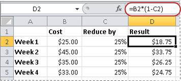
In this formula, 1 is used to represent 100%. Similarly, if you wanted to increase the amount by a certain percentage, you would enter =B2*(1+C2) in D2:
Example 2: Calculate an amount based on a percentage
Scenario If you purchase a computer for $800 and there is an 8.9% sales tax, how much do you have to pay for the sales tax? In this example, you want to find 8.9% of 800.
If B2 is the price and C2 is the sales tax, you can type the formula =B2*C2 in D2, as shown here:
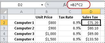
This formula multiplies 800 by 0.089 (the underlying percentage in decimal form) to find the sales tax to pay.
Example 3: Calculate the percentage based on two amounts
Scenario For example, if a student scored 42 points correctly out of 50 on a test, what is the percentage of correct answers?
In this scenario, if the number in B2 is points answered correctly and the number in C2 is the total points possible, you can type the formula =B2/C2 in D2 to find the grade.
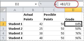
This formula divides 42 by 50 to find the percentage of correct answers. (In the example shown here, the grade is formatted as a percentage without any decimal places showing.)
Example 4: Calculate an amount based another amount and a percentage
Scenario For example, the sale price of a shirt is $15, which is 25% off the original price. What is the original price? In this example, you want to find 75% of which number equals 15.
If B2 is the sale price, and C2 is 0.75, which is 100% minus the 25% discount (in decimal form), you can enter the formula =B2/C2 in D2 to find the original price:
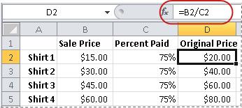
This formula divides the sale price by the percentage paid to find the original price.
Example 5: Calculate the difference between two numbers and show it as a percentage
Scenario For example, the earnings for your department are $2,342 in November and $2,500 in December. What is the percentage change in earnings between these two months? To do this task, use the subtraction (-) and division (/) operators in a single formula.
If B2 represents November earnings, and C2 represents December earnings, you can use the formula =(C2-B2)/ (B2) in D2 to find the difference:
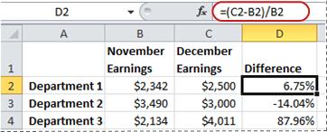
This formula divides the difference between the second and first numbers by the value of the first number to obtain the percentage change. (In the example shown here, the difference is formatted as a percentage with two decimal places.)
Need more help?
You can always ask an expert in the Excel Tech Community or get support in the Answers community.
Источник
Calculate percentages
Sometimes percentages can be frustrating because it’s not always easy to remember what we learned about them in school. Let Excel do the work for you – simple formulas can help you find the percentage of a total, for example, or the percentage difference between two numbers.
Find the percentage of a total
Let’s say that you answered 42 questions out of 50 correctly on a test. What is the percentage of correct answers?
Click any blank cell.
Type = 42/50, and then press RETURN .
The result is 0.84.
Select the cell that contains the result from step 2.
On the Home tab, click  .
.
The result is 84.00%, which is the percentage of correct answers on the test.
Note: To change the number of decimal places that appear in the result, click Increase Decimal  or Decrease Decimal
  .
.
Find the percentage of change between two numbers
Let’s say that your earnings are $2,342 in November and $2,500 in December. What is the percentage of change in your earnings between these two months? Then, if your earnings are $2,425 in January, what is the percentage of change in your earnings between December and January? You can calculate the difference by subtracting your new earnings from your original earnings, and then dividing the result by your original earnings.
Calculate a percentage of increase
Click any blank cell.
Type = (2500-2342)/2342, and then press RETURN .
The result is 0.06746.
Select the cell that contains the result from step 2.
On the Home tab, click .
The result is 6.75%, which is the percentage of increase in earnings.
Note: To change the number of decimal places that appear in the result, click Increase Decimal or Decrease Decimal .
Calculate a percentage of decrease
Click any blank cell.
Type = (2425-2500)/2500, and then press RETURN .
The result is -0.03000.
Select the cell that contains the result from step 2.
On the Home tab, click .
The result is -3.00%, which is the percentage of decrease in earnings.
Note: To change the number of decimal places that appear in the result, click Increase Decimal or Decrease Decimal .
Find the total when you know the amount and percentage
Let’s say that the sale price of a shirt is $15, which is 25% off the original price. What is the original price? In this example, you want to find 75% of which number equals 15.
Click any blank cell.
Type = 15/0.75, and then press RETURN .
The result is 20.
Select the cell that contains the result from step 2.
In newer versions:
On the Home tab, click  .
.
The result is $20.00, which is the original price of the shirt.
In Excel for Mac 2011:
On the Home tab, under Number, click Currency 
The result is $20.00, which is the original price of the shirt.
Note: To change the number of decimal places that appear in the result, click Increase Decimal or Decrease Decimal .
Find an amount when you know the total and percentage
Let’s say that want to purchase a computer for $800 and must pay an additional 8.9% in sales tax. How much do you have to pay for the sales tax? In this example, you want to find 8.9% of 800.
Click any blank cell.
Type = 800*0.089, and then press RETURN.
The result is 71.2.
Select the cell that contains the result from step 2.
In newer versions:
On the Home tab, click .
In Excel for Mac 2011:
On the Home tab, under Number, click Currency
The result is $71.20, which is the sales tax amount for the computer.
Note: To change the number of decimal places that appear in the result, click Increase Decimal or Decrease Decimal .
Increase or decrease a number by a percentage
Let’s say that you spend an average of $113 on food each week, and you want to increase your weekly food expenditures by 25%. How much can you spend? Or, if you want to decrease your weekly food allowance of $113 by 25%, what is your new weekly allowance?
Increase a number by a percentage
Click any blank cell.
Type = 113*(1+0.25), and then press RETURN .
The result is 141.25.
Select the cell that contains the result from step 2.
In newer versions:
On the Home tab, click .
In Excel for Mac 2011:
On the Home tab, under Number, click Currency
The result is $141.25, which is a 25% increase in weekly food expenditures.
Note: To change the number of decimal places that appear in the result, click Increase Decimal or Decrease Decimal .
Decrease a number by a percentage
Click any blank cell.
Type = 113*(1-0.25), and then press RETURN .
The result is 84.75.
Select the cell that contains the result from step 2.
In newer versions:
On the Home tab, click .
In Excel for Mac 2011:
On the Home tab, under Number, click Currency
The result is $84.75, which is a 25% reduction in weekly food expenditures.
Note: To change the number of decimal places that appear in the result, click Increase Decimal or Decrease Decimal .
Источник

A percentage is a kind of fraction saying how many parts over 100 something is. In this article you will see in detail what a percentage is, and how to calculate a percentage in Excel.
First, before diving into how it works in Excel, let’s take a look at the math.
If you want to jump directly to the Excel part, and avoid the math part, please proceed to the section How to work with percentages in Excel.
What is the Formula for Calculating a Percentage?
Percentages from 0% to 100% are equivalent to decimal values from 0 to 1. That means you can convert from a percentage to a decimal number. Let’s see how.
How to Convert from Decimal Number to Percentage
You can convert from a decimal number to a percentage in the following way:
- take the decimal number, (d),
- multiply it by (100),
- and then add the percentage (%) symbol,
In short, if you want to get a percentage from a number (d) you can do this:
[ ( d cdot 100 ) % ]
How to Convert from a Percentage to a Decimal Number
If you want to convert from a percentage to a number, you can:
- take the percentage (P%),
- remove the percentage symbol, (P)
- then divide the number by (100): (frac{P}{100})
In short, to convert a percentage (P%) to a decimal number:
[frac{Pxcancel{%}}{100}]
How to Calculate the Percentage of a Number
There are three cases in which you might want to calculate the percentage of a number:
- to add a percentage to the number (like for calculating how much you have to pay including VAT)
- to just get the percentage of the number
- to subtract a percentage from the number (like for a sale)
How to add a percentage to a number
Let’s first use a specific case, and then let’s generalise.
You went shopping, and the total you need to pay is $185 + VAT. Let’s say VAT in this case is 17%.
So you would have to calculate 17% of $185 and then add it to $185.
[ $185 cdot 17 % + $185 ]
You can make it a single operation if instead you multiply by ( 117 % ).
[ $185 cdot ( 100% + 17% ) = $185 cdot 117% ]
If you have a simple calculator that doesn’t have a percentage operator, you can convert the percentage to a decimal number as we discussed above. Here’s what that would look like:
[ $185 cdot 117% = $185 cdot frac{117 xcancel{ % }}{ 100 } = $185 cdot 1.17 ]
So, in general, if you want to add a percentage ( P % ) to a number ( n ) you can do this:
[ n cdot ( 100% + P%) ]
Or if instead you have the percentage in the decimal number form ( d ) you can do this:
[ n cdot (1 + d) ]
How to calculate the percentage of a number
If you want to buy a house you need to pay a deposit on the house. Let’s say that’s 15% of the total value of the house.
If the house price is $200,000, how can you calculate it?
You can multiply the price by the percent number to get the percentage.
[ $200,000 cdot 15 % = $30,000 ]
So if you want to know what’s the percentage (P%) or fraction (d) of a number (m), you can multiply that number by the percentage or fraction.
[ m cdot P% newline , \ m cdot d ]
How to subtract a percentage from a number
This case is common for calculating the price of an item on sale. For example, if something has an original price of $999 and it is on sale for 20% less, you can calculate the the final price by figuring out what is 20% of $999. Well, it’s $199.80, so then you just subtract that value from $999.
The final price of the item on sale is $799.20.
You can calculate it in a single step if you multiply the original price by ((100% — 20%)) or (80%):
[ $999 cdot (100% — 20%) = $999 cdot 80% = $779.20 ]
So the general formula to subtract a percentage (P%) from a number (b) is:
[ b cdot (100% — P%)]
Or in decimal form:
[ b cdot (1 — d)]
How to Calculate the Percentage of a Number in Respect to Another Number
A cake weights 11 lbs, and you eat 3 pieces for a total of 21 oz. How can you know what percentage of cake have you eaten?
It’s important to do calculations of this kind with everything in the same units. So, first, let’s convert the weight of the cake to ounces.
[ 11~mathrm{lb} cdot frac{16~mathrm{oz}}{mathrm{lb}} = 176~mathrm{oz} ]
Now it’s possible to see the percentage of the cake you’ve eaten: you need to divide the part (in this case the 21 oz of cake you have eaten) by the whole (the 176 oz of the whole cake):
[ frac{11~mathrm{oz}}{176~mathrm{oz}} = 0.0625 ]
As seen in the paragraph on how to convert a decimal to a number, you can convert this to a percentage with ( 0.0625 cdot 100 % = 6.25%).
In this example, you have eaten 6.25% of the whole cake.
How Do You Combine Two Percentages?
Let’s say that some items in an online store are discounted at 20%, and then there is an offer for a 10% discount for everything in your cart at payment.
If you are getting a discount of 20% and then another 10% on top of that… how much is the discount?
It’s not 30%, because the second discount is applied at a different time than the first discount.
A discount of 20% means you pay 80% ((100% — 20%)) of the original price, and a discount of 10% means you pay 90% ((100% — 10%))of the original price. Combining the two discounts means multiplying together the two percentages, like so:
[ 80% cdot 90% = 72% ]
Or in decimal form:
[ 0.80 cdot 0.90 = 0.72 ]
So you pay 72% of the original price, or have a discount of 28%.
Why Are a Decimal and a Percentage Equivalent?
Percentage comes from «per cent», or «over one hundred». The percentage symbol represents the line fraction with 100 in the denominator.
[ 0.20 = frac{20}{100} = 20% ]
The percentage is a simple way to describe how many hundredths of a whole something is.
Now it’s time to start working with Excel. Let’s start with a pretty important thing. How do you write percentages in Excel?
How to Write Percentages in Excel
In Excel you can write percentages in two ways:
- You can write a decimal number and then format the cell as a percentage from the format drop down menu or from the Percent Style button:

- You can write a percentage in the cell, and the cell will automatically take the percentage formatting:

The default format is for a whole percentage. You can change the number of decimal places shown with the «Increase Decimal» and «Decrease Decimal» buttons.

Let’s say you have a decimal form of 0.12345. Formatting it to a percentage will show ( 12% ). You can use the buttons to show the decimal places.

How to Calculate the Percentage of a Number in Excel
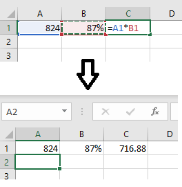
In math, the percentage of a number is calculated by multiplying that number by the percentage: ( 87% cdot 824 = 716.88 ).
In Excel, let’s say you have the number in cell A1 and the percentage in cell B1. To calculate the result, you can write in cell C1 =A1*B1:
How to Calculate the Percentage of a Number with Respect to Another in Excel
In math, you can calculate the percentage of a number with respect to another number by taking the ratio of the two numbers and then converting to a percentage.
If you want to know what percentage 75 is with respect to 142, you can do ( frac{75}{142} = 0.528 = 52.8% ).
Let’s write 75 in cell G1, and 142 in cell H1. To get the percentage of 75 in respect of 142 you can write in cell I1 =G1/H1. The cell will have the result in decimal format, but you can format it to a percentage using the Percent Style button. Then you can adjust the number of decimal places with the Increase Decimal and Decrease Decimal buttons.

How to Calculate a Percentage of Multiple Percentages in Excel
Let’s take the example used above.
An online store has a promotion on some items for 20% off. Then there is another promotion of 10% off for everything in the cart at the moment of payment.
The first discount means you pay 80% of the original price of the item. And then you pay 90% of what’s in the cart.
How much is the discount?
You get the result by multiplying the two percentages. ( 90% cdot 80%).
In Excel, if you have the first percentage in I2 and the second in J2, you can write =I2*J2 to calculate the result.

Conclusion
Percentages are a mathematical tool we use in every day life. In this tutorial, you have learned how they work mathematically, and how to use them in Excel.
I hope this article has been useful.
Learn to code for free. freeCodeCamp’s open source curriculum has helped more than 40,000 people get jobs as developers. Get started
Anyone who constantly works with numbers probably also works with percentages. Calculating percentages apply in many areas of our day-to-day and everyday lives. Some of the areas we apply percentages include; discounts, percentage changes between different values, and percentage of correct answers in a test or survey. Lucky enough, it is easier to calculate percentages. Excel offers you different ways you can calculate percentages just as well as it does with whole numbers and decimals. The Microsoft Excel program e makes it easier by automatically applying simple, basic, or advanced formulas that allow you to add and calculate percentages in your spreadsheet.
In the article below, we will show you how to use the important formulas in excel to calculate percentage changes, discounts, and how to increase and decrease numbers by percentage.
How to calculate percentage basics
A percentage simply means out of 100, that is, a fraction of 100. You calculate it by dividing the numerator by the denominator, and the resulting figure is multiplied by 100. When you are calculating a basic percentage in excel, we use the formula:
= (part/ Total) * 100% or
= Numerator / Denominator * 100%
Remember, just like in all formulas, while calculating the percentage amount, start with an equal (=) sign.
For example, on a 15- day work leaves, Mr. S spent ten days in his hometown and five days in a vacation resort in the USA. What percentage of days did he spend on both places?
The calculations will be as follows:
Percentage formula= part days/ total days * 100%
Percentage of days spent in his hometown = 10/15* 100% = 66.66%
Percentage of days spent in the vacation resort = 5/15* 100% = 33.33%
Hence Mr. S spent 67% of his work leave in his hometown and 33% in the resort.
The example above shows how everyday percentage calculations are done. When computing these calculations using Excel, it is easier as the program performs some of the operations automatically in the background.
Let’s have a look at how percentage calculations in excel will look like;
- To calculate the percentage of the delivered items, you will enter the formula =C2/B2 manually in cell D2. Copying it down the other rows up to cell D9 will give you the decimal results.
- Click on the home tab, and look for the percentage sign in the Number group. After doing this, click on the % icon to display the decimal figures as percentages.
- In case you need to reduce or increase the number of decimal places, you can do so from the home tab in the Number group.

Note;
At times you may have a column full of percentages with many decimal places. We all know this is not standard when presenting data, for example, grades. You can easily reduce the number of decimal places by using the Format Cells feature. Here is what you will do;
- Highlight the column

- Right-click, and from the pop-up menu, select Format Cells to display a pop-up window.

- Click on the Number tab.
- Under the Category menu section, select Number, and click the down arrow that is next to Decimal Places. Click it until you get the desired number of decimal places. In the case above, we clicked up to 0.

- Click OK to display your results in the spreadsheet (the values will be rounded off to the nearest whole number).
How to calculate the percentage of a total in excel
With the above example, we have looked at the different ways you can calculate the percentages of the total. Apart from it, we have different ways one can calculate the percent of a total in excel when you are given different data sets to work with.
Example 1: calculating percentages when part of the total are in multiple rows
Let’s get to understand how this works using the example above. Suppose you have several rows of a product, and you would like to know what percentage of the total is made by orders of the particular product.
In such a scenario, the use of the SUMIF function comes in handy. The function will be used, sum up all the numbers that relate to that given product. The total of all the products will still be used as the denominator. Here is how the formula would be;
=SUMIF (range, criterion, [sum_range]) / total orders
Here is what the percentage calculation will look like in an excel spreadsheet.

In the above table, the formula is applied as follows;
Range A2:A4, the criterion is E1, sum_range B2:B4, and the total orders $B$5
The dollar signs $ creates an absolute reference to cell B10. It means that the value will not change even if the other values change according to the worksheet.
Example 2: calculating the percentage total when the totals of products ordered are provided.
At times you might come across a worksheet that has totals of your data set in a single cell at the end of a table. In such a scenario, to get the percentage of totals, you will use the given total amount as a denominator.
Let’s use the above example without including the number of items ordered.

In the table above, the denominator cell is B10. It is also referred to as the absolute reference cell. To be able to make a cell an absolute reference, you can type in the dollar sign manually or click the absolute reference cell in the formula bar and press F4. This allows you to click and drag down the other rows to get the required percentages.
How to calculate percentage change in excel rows and columns
From mathematics calculations, we all have come across percentage change calculations. When it comes to excelling, it is one of the most commonly used formulas. Percentage change works with both negative and positive values. Here we look at how to calculate percentage increase and decrease in excel.
When you are calculating the percentage change between two values, you use the formula below:
Percentage change = (New value – Old value) / Old value
It is important to take note of which values represent the new and old values when given data sets to work with.
Example 1: calculating the percentage change in an excel spreadsheet
In the example below, suppose you are provided with last month’s prices (January) and this month’s (February) prices in two columns. Then to calculate the percentage change in your excel sheet, you will use the formula below:
= (Current year/week/month value – previous value) / previous value
In our case, we will use the formula = (C2 – B2) / B2

The table above applies to when you have been given values in columns and are expected to calculate the percentage change. What if you are given row data? Sometimes, you may be given data values that relate to particular days of the week, months, or even years to get the percentage change. Therefore, in situations where you have only a column of numbers in an excel sheet, this is the formula to apply:
= (first data cell – second data cell) / second data cell
In our table below, we apply the formula = (B3 – B2) /B2 to calculate the percentage change of sales within a week in January.
Note:
When calculating the percentage growth, we skip the first-row cell of the percentage changes. We do leave it blank because it is not being used in the comparison of the given values.

How to create a custom number format
At times you may want to customize the appearance of numbers. You may decide to make the percentage decrease, which are the negative values to stand out in red. You may also decide to customize your positive values to be green. Here are the steps to follow;
1. Highlight the percentage change column in which you want to apply the customized format.

2. Go to the Home tab, click on the drop-down arrow in the Numbers command group.

3. on the drop-down box, click on the More Number Formats option arrow.
4. In the Format Cells pop-up window, click on the Number tab.

5. Select Custom under the category section. Use one of the existing codes as a starting point to create and save your customized format.
6.
Click OK, and the new format will be applied to the highlighted column.
How to calculate and apply a percentage increase or decrease to values in Excel
At times you may have a budget set aside for certain expenses. Due to unavoidable circumstances, the funds allocated towards the different activities may either increase or reduce. For accountability purposes, you will need to calculate the increase or decrease amounts.
To increase an amount by a percentage, apply the formula below:
= Amount * (1 + % increase)
To decrease a current amount by percentage, use the formula
= Amount * (1 – % decrease)
Let’s have a look at how you can increase or decrease given values by a percentage.
Example:
Suppose you have been given a column of sales value you are supposed to increase or reduce by a certain percentage. It is good to have the updated values in one column rather than have a different column where the formula appears.
Let’s look at the steps to be followed to arrive at the expected results.
1. In one column, enter all the sales amount values you want to increase or decrease.

2. enter the formula that applies in an empty cell. That is, enter either the increase or decrease formula.

3. Select the cell with the formula and copy it. You can use the shortcut Ctrl + C or by right-clicking and selecting Copy.
4. Select the range of cells you want the increase or decrease applied to.
5. Right-click the selected cells and then click on the Paste Special feature to display a dialog window.
6. In the Window, under the paste category, select Values. In the Operation category, select multiply.
7. Click OK to display your results.

Note;
We use parentheses in the formula when calculating any percentage changes due to an increase or decrease in a given amount. By default, Excel operations state that multiplication must be done before addition or subtraction. Letting this happen in the above formula may lead to you getting the wrong results. Therefore, as in the formula, the second part is wrapped in parentheses to ensure that the multiplication part is calculated last.
Calculating and finding percentiles in excel
When working with percentages, you may have to calculate the percentile rank of a given data set. The percentile rank of a given number is where it falls in a range of different numbers. In excel, it is easier to calculate percentile rank as there are functions available to make your work easier. The two functions in excel are:
=PERCENTILE. EXC (array, value)
=PERCENTILE. INC (array value)
The functions above include the same arguments. These are:
- Array- this argument is the range of numbers that you are looking for in a percentile.
- Value-this argument represents the percentile rank you are looking for.
Example
Suppose you are given percentage scores of a class. Find the 60th percentile.
To get the solution below, we use the formula =PERCENTILE.INC (B2:B5, .6)

How to calculate the Discount Rate or Price in Excel spreadsheets
During special occasions globally, most sellers and supermarkets always offer their products at discounts. It may be Christmas, Easter, or Thanksgiving holiday, or it may be an anniversary for the shop. So you may get as high as a 70% discount to as low as a 100% discount. But what if you plan on purchasing a lot of products offered at a discount and you need to know the different discount rates and prices you will pay? There is no reason to be frustrated as with excel, and you can easily calculate the discount rates and prices.
Here is a step-by-step guide on how to calculate discount rates in excel when given the initial price and the current selling price.
1. In an excel worksheet, in one column, type in the initial price values of the product. In the second column, you will type in the current sales price, while the third column will be discount rates.

2. To get the discount rate of the first product, type in the empty cell the formula = (C2-B2)/B2. Where B2 indicates the original price, C2 represents the current sales price.

3. Press the Enter button to get the resulting discount rate of that product. To fill in the other blanks, drag the fill handle to fill the above formula to the other empty cells.
4. Remember, your values will be in decimal places, and therefore, you will need to convert them into percentages and adjust the number of decimals.

What if you have been given the discount rate as it is on many occasions and told to calculate the current selling price of an item?
Follow these steps
1. Select the first blank cell on the selling price column.
2. Type in the formula =B2- (B2*C2) where B2 represents the original price, and C2 is the discount rate of each item.

3. Press the Enter button and drag the fill handle to fill in the other empty cells. The selling price figures will be shown in the empty cells as shown below.

How to calculate percentage profit in Excel
When we talk about profits, we refer to the financial benefits that a business or company remains with after paying all its expenses. Profit percentage calculation is an important tool in any business setting. It is a common tool as it helps measure the profitability of a business. A business uses the percentage to measure its ability to convert its sales into profits. A company also uses profits to gauge the capacity of a business to continue its operations in the foreseeable future. Therefore, it is a vital computation in any business. Profit is calculated and expressed as a percentage of the selling price. In Excel, there are two types of profit percentages;
- Profit margin-it is the percentage you get on the selling price. The formula is;
Profit Margin = (Profit/ Cost Price) * 100
- Markup- it is calculated as the percentage of the cost price. The formula is;
% Markup = (Profit/ Cost Price) * 100
Example: Excel profit percentage calculation
Suppose you are the owner of a retail shop, and due to the heavy demand during the Christmas season, you purchase 150 pieces of refrigerated turkey at the rate of 35 per bird. You also purchase 80 bottles of wine at the rate of 115 per bottle. Due to the high costs of transportation expenses incurred, $2500, you decide to sell the turkey at $50 per bird and a wine bottle at $150. Apart from this, you offer your customers a discount of 5% on any product purchased from your retail shop. What will be your total profit on the two products?
Here are the steps to be followed to get the profit amount;
- To get the profit, you first have to calculate the total sales and cost. We use the formula ;
Profit = Total Sales- Total Cost
In our excel spreadsheet, the total cost will be the sum of the transportation costs, the turkey’s total cost, and the wine’s total cost. The total sales will be the sum of the net sales of the turkey and the net sales of the wine. When you want to get the net sales, we will minus the discount rate amount from the selling price. To get the profit as in our figure below, we use the formula = B10-B5.

- To get the percentage profit, we use the formula = (Profit/ Total cost) * 100. From the example above, our formula will be
Profit % = (B12/B5) *100

Conclusion
As seen above, Microsoft Excel formulas for percentages are crucial in our everyday life. Even if percentages have never been your favorite calculations to perform, with the above basic excel formulas, you can hack them and get excel to do your computations. Take note that these are just some of the basic excel percent formulas. You can also decide to dive into the advanced percentages like variance, interest rates percentage, etc.
How to Calculate Percentage Using Excel Formulas?
The percentage is calculated as the proportion per hundred. In other words, the numerator is divided by the denominator and the result is multiplied by 100. The percentage formula in Excel is = Numerator/Denominator (used without multiplication by 100). To convert the output to a percentage, either press “Ctrl+Shift+%” or click “%” on the Home tab’s “number” group.
Let us consider a simple example.
On a 15-day vacation, Mr. A spent 10 days in his hometown and 5 days in the USA. What percentage of days did he spend in the USA?
The calculations are given as follows:
- Percentage formula=Portion days/Total days*100
- Percentage of days spent in the USA=5/15*100=33.33%
- Percentage of days spent in hometown=10/15*100=66.66%
Hence, Mr. A spent approximately 33% of his vacation period in the USA.
Table of contents
- How to Calculate Percentage Using Excel Formulas?
- Example #1
- Example #2
- Example #3
- Frequently Asked Questions
- Recommended Articles
You can download this Formula for Percentage Excel Template here – Formula for Percentage Excel Template
Let us go through the following examples to understand the concept of percentage in Excel.
Example #1
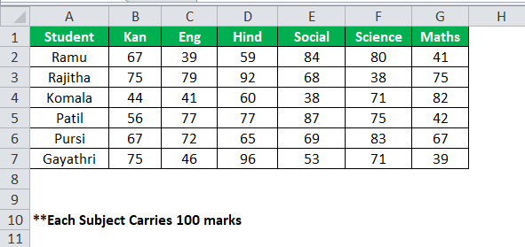
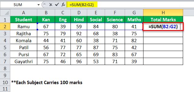
The following table shows the subject-wise marks of 6 students in a school. Since the results pertain to the annual examinations, the maximum marks of every subject are 100.
We have to calculate the percentage of marks for all students.
The steps to calculate percentages in Excel are listed as follows:
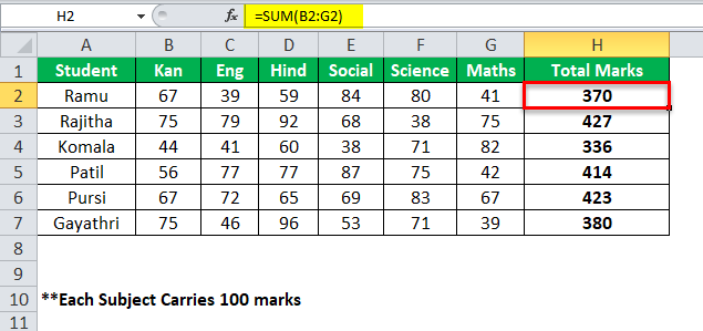
- Calculate the total marks obtained by the students. For this, the marks of every subject are added.

- Drag the formula of cell H2 to get the total marks obtained by all students. The output is shown in the following image.

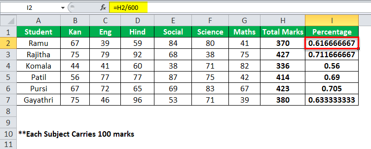
- Divide the total marks by 600. The values of the “total marks” column become the numerator. Since the number of subjects is 6, the maximum marks are 600 (100*6=600). This becomes the denominator.

- Apply the following formula.
Percentage=Marks scored/Total marks*100.
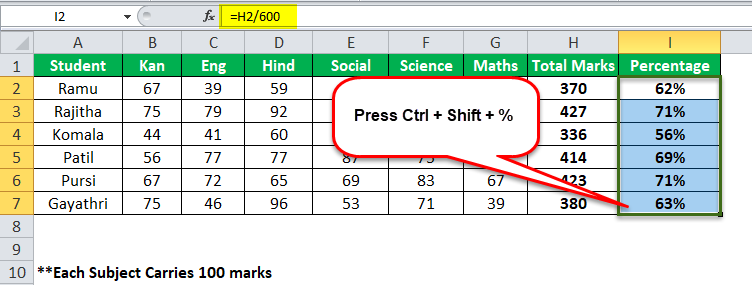
For percentage values (shown in the succeeding image), change the cell formatting. Select column I and press “Ctrl+Shift+%.” Alternatively, select “%” in the “number” group of the Home tab.

Example #2
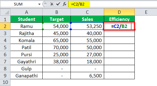
The following table consists of students who undertake internship in an organization. Their task is to sell products based on pre-defined targets.
We want to determine the efficiency level (percentage) of every student.

The steps to calculate the efficiency level are listed as follows:
Step 1: Apply the formula “sales/target.”
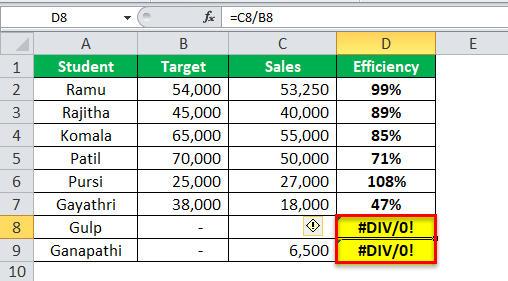
Step 2: Format column D to obtain the efficiency levels in percentage. For the last two students (Gulp and Ganapathi), the formula returns “#DIV/0!” errorErrors in excel are common and often occur at times of applying formulas. The list of nine most common excel errors are — #DIV/0, #N/A, #NAME?, #NULL!, #NUM!, #REF!, #VALUE!, #####, Circular Reference.read more.
Note: If the numerator is zero, the division of the numerator by the denominator returns “#DIV/0!#DIV/0! is the division error in Excel which occurs every time a number is divided by zero. Simply put, we get this error when we divide any number by an empty or zero-value cell.read more” error.
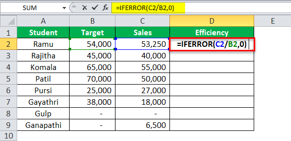
Step 3: To eliminate the error, tweak the existing formula as “=IFERROR(C2/B2,0).” This implies that the IFERROR The IFERROR function in Excel checks a formula (or a cell) for errors and returns a specified value in place of the error.read moredisplays zero if the division of C2 by B2 returns an error.
In other words, the “#DIV/0!” error is replaced by zero with the help of the modified formula.
Note: The IFERROR functionThe IFERROR function in Excel is used to determine what to do when an error occurs before performing any function.read more helps get rid of percentage errors.
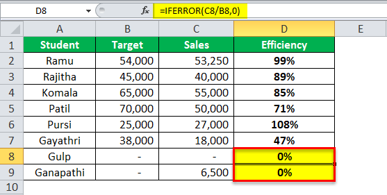
Step 4: The output using the IFERROR function is shown in the following image. The efficiency levels of students Gulp and Ganapathi are zero. This is because of the blank (zero) in column B and/or column C.
Example #3
For 2018, an organization’s sales for the months January and February are given in the following table.
We want to calculate the growth or the decline (percentage) in monthly sales.
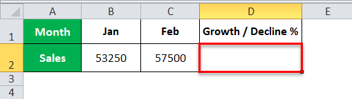
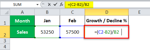
The steps to calculate the increase (growth) or decrease (decline) percentage are listed as follows:
Step 1: Apply the formula “=(C2-B2)/B2.”
The sales in February (57500) are more than the sales in January (53250). The difference (growth) between the two sales is divided by the sales of the initial month (January).
Step 2: Format column D to obtain the growth percentage.
Hence, the February sales have increased by 7.98% over January sales.

Note: While calculating the growth or decline percentage, if the numerator or the denominator is less than zero, the output is a negative value.
Frequently Asked Questions
1. What is the Excel formula for percentage?
The basic percentage formula is “(part/total)*100”. This formula is used in Excel without the latter part (*100). This is because when the percentage format is selected, the resulting number is automatically changed to percent.
In addition, the decimal points are removed and the output is shown as a rounded percentage. For instance, 26/45 is 0.5777. By applying the percentage format, this decimal number becomes 58%.
To convert the output to percentage, either press “Ctrl+Shift+%” or select “%” in the “number” group of the Home tab.
2. What is the Excel formula for calculating the percentage change?
The formula for calculating the percentage change is stated as follows:
“(New value-Initial value)/Initial value”
This formula helps calculate the percentage increase or decrease between two values. A positive percentage implies an increase, while a negative percentage shows a decrease.
Note: To get the final answer (percentage change), the percentage format is applied to the output of the formula.
3. What is the Excel formula for calculating the percentage of the total?
The formula for calculating the percentage of the total is “(part/total).” For instance, column A lists the monthly expenses from cell A2 to cell A11. The cell A2 contains $2500 as the rent paid. The cell A12 contains the total expenses $98700.
The formula “=A2/$A12” returns 3% after applying the percentage format. This implies that the rent is 3% of the total paid expenses.
Since A2 should change on dragging the formula to the remaining cells, it is entered as a relative reference. On the other hand, the total should remain fixed for all cells, so A12 is entered as an absolute reference.
- The percentage is the proportion per hundred.
- To calculate the percentage, the numerator is divided by the denominator and the result is multiplied by 100.
- For obtaining percentages, the output column is formatted by pressing “Ctrl+Shift+%” or selecting “%” in the Home tab.
- The division of the numerator by the denominator returns “#DIV/0!” error if the former is zero.
- The percentage errors can be removed with the help of the IFERROR function.
- The increase or decrease percentage is calculated by dividing the difference between two numbers with the initial number.
Recommended Articles
This has been a guide to formula for percentage in Excel. Here we discuss the calculation of Excel percentages using the IFERROR formula along with Excel examples and downloadable Excel templates. You may also look at these useful functions in Excel –
- Percentage Change Formula
- Percentage Profit Formula
- Calculate the Percentage Increase in Excel
- Percentage Difference in Excel
We often have to work with percentages in our day-to-day work and our everyday life. Excel makes this task easier by automatically applying basic or advanced formulas that allow you to calculate percentages directly in your spreadsheets. We’ll show you how to use the most important formulas in Excel to calculate percentages of totals or percentage changes such as growth and decline. You’ll also learn how to calculate proportions and totals based on percentages and how to increase and decrease numbers by percentage.
Contents
- Calculating percentages in Excel – the basics
- Calculating percentages in Excel – formulas and formatting
- Adding percentage formatting in Excel
- Adjusting percentage formatting in Excel
- Calculating the percentage of a total in Excel
- Calculating the percentage of a total at the end of an Excel table
- Calculating percentages of a total from different rows
- Formula for calculating a percentage change in Excel
- Calculating the percentage of change between two columns
- Calculating the percentage of growth between two rows
- Calculating the proportion and the total based on a percentage in Excel
- Calculating the proportion based on the total and based on percentages
- Calculating the total based on the proportion and percentage
- Increasing and decreasing numbers by a percentage in Excel
$1 Domain Names
Register great TLDs for less than $1 for the first year.
Why wait? Grab your favorite domain name today!
![]() Matching email
Matching email
![]() SSL certificate
SSL certificate
![]() 24/7/365 support
24/7/365 support
Calculating percentages in Excel – the basics
In this article, we’ll give you an overview of the most important methods for calculating percentages in Excel and show you the most important formulas for doing percentages.
Tip
Microsoft Excel can help you with many basic and advanced calculations in your day-to-day work. Learn more about the SUM function in Excel if you want to easily add groups of numbers.
The word “percent” is of Latin origin and means “by a hundred”. In other words, you calculate a percentage by dividing the numerator of a fraction by the denominator and multiplying the result by 100. The basic formula for calculating apercentage looks like this:
(Part/Total)*100=PercentageFor example, if you sell a product for $14 that costs $10.50 to manufacture, the manufacturing cost is 75 percent of the total price. We often use this formula to calculate percentages in our everyday lives. However, with Excel, calculating percentages is even easier because the spreadsheet application automatically performs several steps in the background.
Tip
Organize your data in Excel, create spreadsheets, and calculate your expenses, profits, and much more. Get the spreadsheet program as part of the Microsoft 365 package directly from IONOS and get optimum round-the-clock support for Microsoft Excel and other Office products.
Calculating percentages in Excel – formulas and formatting
When you calculate percentages in Excel, you’ll save yourself steps like multiplying by 100 because the application automatically handles the formatting for you once you apply the percent format (see below for more information). The formula for calculating percentages in Excel is as follows:
Let’s look at a practical example of how percentages are calculated in Excel: A retailer uses a spreadsheet of purchased and sold products in order to keep track of inventory. The number of products that the retailer buys is in column B and the number of products that the retailer sells in is column C. To calculate the percentages in column D of the Excel spreadsheet, enter the following formula (and then press Enter):

You can easily apply the formula to subsequent rows by double-clicking the bottom right corner of the cell (in this case: D2). Excel also automatically adds the formula as you enter more data in columns B and C.
Adding percentage formatting in Excel
However, the results may not look quite right at first: Instead of percentages, you’ll see decimal numbers in your Excel spreadsheet.

If you want Excel to automatically add the percent sign and round up to the percentage using the formatting, you have to adjust the following settings first: To quickly change the cell format to show values as percentages in Excel, go to the “Number” group (between “Alignment” and “Styles”) on the “Home” tab. Once there, simply click the percent sign to select the percent format – either for a single cell, a range of cells or an entire column or row. In this case, we calculated percentages in column D of our Excel spreadsheet by selecting the appropriate cells beforehand:

Alternatively, you can use the keyboard shortcut Ctrl + Shift + % (as shown in the screenshot above) to enable the percentage format.
Adjusting percentage formatting in Excel
If you follow the steps above, percentages are displayed without decimal places according to the default settings in Excel. However, you can change the percentage formatting in Excel simply by clicking the little arrow icon at the bottom right in the “Number” group. Alternatively, you can select a cell and right-click it to display the “Format cells” dialog box.
To adjust the percentages in Excel, you can then specify the number of decimal places you want to display. For example, to display two digits after the decimal point, select “2”. Then click OK.

Alternatively, you can choose the “Custom” category in the same dialog box to specify percentages either without a decimal place or with two decimal places.

Note
Formats in Excel not only help you calculate percentages; you can also use them for many other processes and tasks. For example, in another article we explain how to calculate time in Excel.
Calculating the percentage of a total in Excel
In the examples above, we calculated percentages of a total. The purchases and sales are the total and the sales are the percentages. However, we can also use Excel to do more complicated calculations for finding the percentages of a total.
Calculating the percentage of a total at the end of an Excel table
Let’s say the retailer in the example above now wants to know how many products they purchased in total and what percentage of the total purchase amount is attributed to each product. Excel works out the percentage of the total that each amount represents. However, first we have to determine the total quantity of all products in cell B11. In the column to the right, we use Excel to find out what percentage of the total each product represents. To do this, we enter the following values in cell C2 or select these values with the mouse button:

The $ signs create an absolute reference to cell B11. This means that the value does not change even if the other values change according to the spreadsheet. For example, “=B3/$B$11” appears in cell C3 after the formula from cell C2 is automatically applied. Without the absolute value, which is indicated by the dollar sign, “=B3/B12” would appear in this cell and the example formula would not calculate any percentages because cell B12 is empty.
Note
You can also define a cell as an absolute value by pressing the [F4] key on your keyboard after you have selected the cell with the mouse or entered it manually.
Calculating percentages of a total from different rows
Now let’s say the retailer has multiple rows for the same product and wants to use Excel to find out what percentage of the total that product represents. In this case, you can use the SUMIF formula, which automatically adds all values that match the criteria you have selected. Combined with the SUMIF formula, the complete formula for calculating percentages in Excel looks like this:
=SUMIF(range,criteria,sum_range)/totalIn our example, we entered the criteria “Pants” in cell E1. The values that we want to add are in column B and the product names for automated selection are in column A. The corresponding formula in Excel is as follows:
=SUMIF(A2:B10,E1,B2:B10)/$B$11Here’s how it looks in the Excel spreadsheet:

Instead of specifying your criteria in a cell of your Excel spreadsheet, you can type it directly into your formula, which then reads “SUMIF(A2:B10,»Pants»,B2:B10)/$B$11”. You can also use parentheses to work with multiple SUMIF functions, for example, to calculate percentages of multiple products in Excel:
=(SUMIF(A2:B10;"Pants",B2:B10)+SUMIF(A2:B10,"Shirts",B2:B10))/$B$11))Formula for calculating a percentage change in Excel
The percentage of change or percentage of growth is probably one of the formulas that you’ll use most often when you calculate percentages in Excel. Simply use the following formula to calculate the change between the original value A and the value B:
Percentage change=(B-A)/AThe original value A represents the value before the change. For example, if you compare sales between the two months of March and April, the number of sales in March would be the original value A and sales in April would be B. The following two examples illustrate how to calculate the percentage of growth using this formula.
Calculating the percentage of change between two columns
The retailer in our example entered the sales from March in column B and the sales from April in column C. The retailer then enters the following formula in column D to calculate the percentage of growth:
Note
Don’t forget: After this step, you have to format the cells in column D as percentages so that the result is displayed correctly.
 in Excel")
Calculating the percentage of growth between two rows
You may want to keep track of total monthly sales in a spreadsheet. In this case, you can calculate the percentage of growth between two rows so that you can easily see month-over-month changes in sales. In the example, we enter all monthly sales in column B and calculate the growth in column C. Start with the sales from January in cell B2 and determine the percentage of growth for February in cell C3. To do this, enter the following formula in cell C3:
Then apply the formula to the subsequent rows (starting with C4). In your Excel spreadsheet, you can see the percentage of growth as follows:

When you calculate the percentage of growth, be sure to leave the first row blank because it is not being used in the comparison. In this example, you are not comparing January to the prior month.
You can also calculate the percentage of growth in Excel in comparison to a static value that does not change. To do this, simply enter the absolute reference to the cell by pressing the F4 key and adding the $ sign as explained above.
Calculating the proportion and the total based on a percentage in Excel
Just as you can use Excel formulas to calculate percentages based on two values, A and B, you can also calculate a total or the proportions of a totalbased on a percentage.
Calculating the proportion based on the total and based on percentages
Let’s say you buy new IT equipment for your company and the total price is $1,200. This includes sales tax, which may be tax-deductible. Sales tax varies from state to state, so for the sake of illustration let’s assume that you live in Wisconsin, where sales tax is 5%. For this purpose, you simply calculate the amount of sales tax based on the percentage. In the following example, the total price is in cell A2 and the percentage is in cell B2. You need to calculate the absolute value of the sales in cell C2. The appropriate formula is:
The result: The purchase price includes $60 of sales tax.

Tip
If you don’t want to enter the percentage in a separate cell, you can also integrate it directly into the formula. Enter either “=A2*5%” or “=A2*0.05”.
Calculating the total based on the proportion and percentage
Excel also allows you to calculate a total based on the proportion and percentage. For example, let’s say you attend a multi-day workshop in another city. As a workshop attendee, you receive a special discount and pay only 70 percent of the price of your hotel room as part of your all-inclusive accommodations. You are charged $350 and are curious how expensive your stay would have been without the discount.
Enter the amount you paid in cell A2 and the percentage in cell B2. In cell C2, enter the formula for calculating the total price based on percentages. Divide your amount by the percentage:
If you entered everything correctly, you’ll see that the hotel price would have been $500 without the discount:

Increasing and decreasing numbers by a percentage in Excel
You can also use percentages to increase and decrease numbers in Excel. This is especially useful for our retailer in the previous examples. For example, if the retailer wants to increase all prices by 20 percent to compensate for increased expenses, they can use the following formula:
The retailer can then reduce the prices again during the end-of-season sale. Note that Excel also recognizes the decimal notation when calculating the percentage:
In the example, a price increase looks like this: Column A shows the product type and column B shows the current price. To calculate the new price in column C, the retailer uses the following formula:
The retailer now sees the new prices, which are 20 percent higher, in column C:
