
This is going to be a trouble-shooting tutorial where we are going to focus on what to do if you can’t type into a cell in Excel (i.e., you type but don’t see anything getting typed in the cells).
An issue like this can be quite frustrating, especially if the work is important or urgent.
If you’ve run into a problem like this, this tutorial will help you diagnose the probable cause of the problem and how to rectify it step-by-step.
We are going to assume you have already tried restarting your computer and have checked if your keyboard is properly connected and working, but have still not been able to solve the issue.
Let us look at some common reasons for not being able to type in Excel.
Once you are able to trace the cause, it becomes easier to decide on the next steps to solve the problem.
Here are some possible reasons you can’t type in Excel, along with their respective solutions.
Your cells may have Font Color set to White/Text may be Invisible
If you type into a cell and see the cursor move but nothing appears in the cell, then it’s probably because your font color and cell background color are the same and so your text is basically camouflaged.
In such cases, you will also notice the text appearing in the formula bar, but not in the cells.

Solution:
The solution to this problem is quite simple.
Just change the font color or background color!
Alternatively, you can remove all formatting from the cell by clicking on the Home tab and navigating to Cell Styles->Normal from the Styles group.
Alternatively, you can select the ‘Automatic’ font color from the Font group in the Home tab.

Also read: Can’t Insert a Row in Excel – How to Fix!
Your Num Lock may be Preventing You from Entering Numbers
If you’re trying to enter numbers from your num pad, and you find yourself unable to type into a cell, a possible cause might be that your num lock is turned off.
The num lock (or Number lock) is a toggle key on your keyboard that lets you control the use of the numeric keys in the num pad (the set of the numbers on the right side of your keyboard).
Notice that each number key in your num pad has two different functions.
For example, the number 7 doubles up as the Home key, while the number 8 doubles up as the Up arrow key.
When the num lock is off, you can use the num pad like a regular numeric pad.
However, when it is off, it locks the numbers, letting you use the other functions that the number keys are associated with.
Most keyboards have a small LED on top of the num lock, which lights up when the num lock is on. Check to see if the num lock LED is not on. If so, then it’s probably the reason you are unable to type numbers into your cell.
If your keyboard does not have an LED or any other indicator to show if the num lock is on, just try typing some text into the cell.
If you are able to type text but not numbers, it could indicate an issue with your num lock.
Solution:
To turn the num lock on, simply press the Num lock button again.
This will cause the lock to toggle off and you can start typing numbers from the num pad again!
The Cells Could be Locked or Protected
If your worksheet is in ‘Protected’ mode, then all the cells of the sheet become read-only.
This usually happens when the author of the worksheet chooses to protect the contents of cells on the sheet from changes by unauthorized people.
To check if that’s the case, go to the Review tab. If you see a button that says ‘Unprotect Sheet’ and/or ‘Unprotect Workbook’, it means your sheet is in Protected mode.

Moreover, when you try to edit or type into any cell, you should see an alert that says ‘The chart or cell you are trying to change is on a protected sheet’.

Solution:
You can disable protection by simply clicking on the ‘Unprotect Sheet’ and/or ‘Unprotect Workbook’ button.
If the sheet is protected with a password, then you might need to get it from the sheet’s author in order to disable protection.
The Cell May have Validation Rules Applied to It
Validation rules are usually applied to cells to allow certain specific values or types of values to be entered.
For example, the author might apply a validation rule to restrict a cell to only allow numeric values or values within a certain boundary.
When you try to enter a value into that cell that breaks the validation rule, you will usually not be allowed to enter it, and an error message appears.

Solution:
The solution to this is to either enter a number that is in line with the validation rule, or to remove the validation rule from the cell altogether.
To remove the validation rule, select the problematic cell(s) and navigate to Data->Data Validation.
This will open the Data Validation dialog box from where you can see the validation rule(s) applied to your selected cell(s).
To remove the validation rule, simply click on the Clear All button. Then Click OK to close the dialog box.

Cell Values May be Hidden
Your cell might be set to ‘Hidden’ format, preventing your typed text from appearing in the cell when you press the return key after typing.
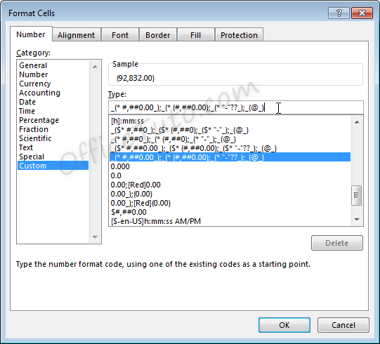
To check if your cell is set to the ‘Hidden’ format, right-click on it and select Format Cells.
Alternatively, you could select the problematic cell(s) and press the keyboard shortcut CTRL+1.
This will open the Format Cells dialog box. Select the Number tab and under the Category list, select Custom.
Check the input box under ‘Type’. If you see three semicolons (;;;) it indicates that the cell(s) have been formatted as hidden cells.

Solution:
To unhide your cell values, simply remove the three semicolons from the Format Cells dialog box and click OK.
Certain Add-ins might be Preventing you from Typing
If you’ve recently installed a new add-in to Excel, it might be interfering with your current install, causing your Excel software to act up.
If none of the above-mentioned issues seem to be the cause, then this could be a probable reason for not being able to type in Excel.
To check if an add-in is causing your problem, try to re-open Excel in ‘Safe mode’.
Opening Excel in Safe mode disables all add-ins, leaving you with just the bare basics.
This helps you narrow down to the exact source of the problem, and is a widely used trouble-shooting method.
To open in Safe mode, follow the steps shown below:
- Close the Excel Window
- Press the Windows key+R shortcut to open the ‘Run’ box.
- In the input box next to ‘Open’, type ‘Excel/safe’.

- Click OK.
Microsoft Excel should now open in Safe mode. If you find your issue resolved now, it means one of your add-ins was causing the problem.
Solution:
Once you know that an add-in is behind the problem, you can now attempt to narrow down to exactly which add-in it is and disable it. Here’s how:
- Navigate to File->Options
- From the Excel Options dialog box, select Add-ins
- At the bottom of the box, you’ll find a dropdown next to ‘Manage’.

- Select COM Add-ins from this dropdown list.

- Click Go.
- You should now see a list of installed add-ins.
- Click any one of the checkboxes and click OK. This will make sure that only the checked add-in is active the next time you open Excel while all others are disabled.
- Close and restart Excel.
- Try typing something into a cell. If you see your problem resolved, it means your previously selected add-in was not causing the problem. Try activating another add-in. Repeat until you find exactly which add-in caused the issue.
Note: Make sure you close and restart Excel each time you activate an add-in.
In this tutorial, we discussed possible reasons you can’t type in Excel and showed you how to solve the problem in each case.
We hope we were able to help you successfully eliminate the problem and start typing in Excel again.
Other articles you may also like:
- Why does Excel Open on Startup (and How to Stop it)
- How to Remove Read-Only From Excel (6 Easy Fix)
- Why is Merge and Center Grayed Out?
- How to Open Excel File [xls, xlsx] Online (for FREE)
- How to Find out What Version of Excel You Have
- How to Set the Default Font in Excel (Windows and Mac)
- SPILL Error in Excel – How to Fix?
- Circular References in Excel – How to Find and Fix it!
- Excel Shortcuts Not Working – Possible Reasons + How to Fix?
- #NUM! Error in Excel – How to Fix it?
Some users are experiencing an issue with Excel. According to them, they are not able to type in any of the cells in an Excel spreadsheet. Also, there are no macros enabled and the Excel sheet or cells are not protected. If you are unable to type in Excel, you can refer to the solutions listed in this article to get rid of the problem.

The troubleshooting guidelines to deal with this problem are explained below. But before you proceed, close all the Excel files and open Excel again. Now, check if you can type something in your Excel spreadsheet. If Excel won’t let you type this time too, restart your computer and check the status of the issue.
Some users were able to fix the problem by doing the following trick:
- Open a new blank Excel spreadsheet.
- Type something in the new spreadsheet.
- Now, type in the original (problematic) spreadsheet.
You can also try the above trick and check if it helps. If the issue persists, try the following fixes.
- Check the Editing options setting
- Troubleshoot Excel in Safe mode
- Move files from the C directory to another location
- Uninstall the recently installed software
- Disable the Hardware Graphic Acceleration in Excel
- Change the Trust Center settings
- Repair Office
- Uninstall and reinstall Office
Below, we have explained all these fixes in detail.
1] Check the Editing options setting
If the “Allow editing directly in cells” option is disabled in Excel Editing settings, you may experience this type of problem. To check this, go through the following instructions:

- Open Excel file.
- Go to “File > Options.”
- Select Advanced from the left pane.
- The “Allow editing directly in cells” checkbox should be enabled. If not, enable it and click OK.
2] Troubleshoot Excel in Safe mode
The problem might be occurring due to some Excel Add-ins. You can check this by troubleshooting Excel in Safe mode. Some of the Add-ins remain disabled in the Safe mode. Hence, launching an Office application in Safe mode makes it easier to identify the problematic Add-in.
The process to troubleshoot Excel in Safe mode is as follows:
- Save your spreadsheet and close Excel.
- Open the Run command box (Win + R keys) and type
excel /safe. After that click OK. This will launch Excel in the Safe mode. - After launching Excel in Safe mode, type something in cells. If you are able to type in the Safe mode, one of the Add-ins disabled in the Safe mode by default is the culprit. If you are unable to type in the Safe mode, one of the Add-ins enabled in the Safe mode is the culprit. Let’s see these two cases in detail.
Case 1: You are able to type in the Safe mode
- In the Safe mode, go to “File > Options.”
- Select Add-Ins from the left side.
- Now, select COM Add-ins in the drop-down and click Go. After that, you will see all the Add-ins that are enabled in the Safe mode. Because you are able to type in the Safe mode, none of these Add-ins is causing the problem. Take a note of the Add-ins that are enabled in the Safe mode.
- Close Excel in the Safe mode and open Excel in the normal mode.
- Go to “File > Options > Add-Ins.” Select COM Add-ins in the drop-down and click Go.
- Disable any of the enabled Add-ins and click OK. Do not disable the Add-ins that were enabled in the Safe mode.
- After disabling an Add-in, restart Excel in normal mode and check if you are able to type. If yes, the Add-in that you have disabled recently was causing the problem. If not, repeat steps 5 to 7 to identify the problematic Add-in. Once you find it, consider removing it.
Case 2: You are unable to type in the Safe mode
- In the Safe mode, go to “File > Options > Add-Ins.” Select COM Add-ins in the drop-down and click Go.
- Disable any of the Add-ins and click OK.
- Now, type something. If you are able to type, the Add-in that you have disabled recently was causing the problem. Remove that Add-in.
- If you are unable to type, disable another Add-in in the Safe mode and then check again.
3] Move files from the C directory to another location
Move the Excel files from the C directory to another location and check if the problem disappears or not. Follow the instructions listed below.
- First, close Excel.
- Open the Run command box and type
%appdata%MicrosoftExcel. Click OK. This will open the Excel folder in your C drive. It is a temporary location for unsaved files. Excel saves your files here temporarily so that they could be recovered in case Excel crashes or your system shuts down unexpectedly. - Move all the files to another location and make the Excel folder empty. After that, open Excel and check if the problem disappears. If this does not fix the issue, you can place all the files back in the Excel folder.
4] Uninstall the recently installed software
If the problem started occurring after installing an app or software, that app or software may be the cause of the problem. To check this, uninstall the recently installed app or software and then check if you can type in Excel. Some users have found the following third-party applications the cause of the problem:
- Tuneup Utilities
- Abby Finereader
If you have installed any of the above software, uninstall them and check if the problem disappears.
Read: Excel freezing, crashing or not responding.
5] Disable the Hardware Graphics Acceleration in Excel
If the Hardware Graphics Acceleration is enabled in Excel, that may be causing the problem. You can check this by disabling the Hardware Graphics Acceleration. The steps for the same are as follows:

- Open Excel.
- Go to “File > Options.”
- Select the Advanced category on the left side.
- Scroll down and locate the Display section.
- Uncheck the Disable hardware graphics acceleration checkbox.
- Click OK.
6] Change the Trust Center settings
Change the Trust Center settings and see if this fixes the issue. The following steps will help you with that.

- Open Excel.
- Go to “File > Options.” This will open the Excel Options window.
- Select the Trust Center category from the left side and click on the Trust Center Settings button.
- Now, select Protected View from the left side and uncheck all the options.
- Select File Block Settings from the left pane and uncheck all the options.
- Click OK to save the settings.
7] Repair Office
If despite trying all the above fixes, the problem still persists, some of the Office files might be corrupted. In such a case, an Online Office Repair may fix the problem.
8] Uninstall and reinstall Office
If the online repair fails to fix the problem, uninstall Microsoft Office and install it again. You can uninstall Microsoft Office from the Control Panel or from Windows 11/10 Settings.
Read: How to fix high CPU usage by Excel.
Why is my Excel not allowing me to type?
There are several reasons why Excel is not allowing you to type, like incorrect Editing settings, conflicting apps or software, etc. Apart from that, problematic Add-ins also cause several issues in Microsoft Office applications. You can identify which Add-in is causing the problem by troubleshooting Excel in the Safe mode.
Sometimes, the Hardware Graphics Acceleration or Protected view causes problems in Excel. You can change the Trust Center settings and see if this fixes the problem.
If some Office files get corrupted due to some reason, you may experience different errors in different Office applications. Such a type of problem can be fixed by running an online repair.
How do I unlock my keyboard in Excel?
If you turn on Scroll Lock in Excel, you can move the entire sheet by using the arrow keys. To unlock your keyboard in Excel, turn off the Scroll Lock.
Hope this helps.
Read next: Fix Errors were detected while saving the Excel file.
Enter data manually in worksheet cells
Excel for Microsoft 365 Excel 2021 Excel 2019 Excel 2016 Excel 2013 Excel 2010 Excel 2007 More…Less
You have several options when you want to enter data manually in Excel. You can enter data in one cell, in several cells at the same time, or on more than one worksheet at once. The data that you enter can be numbers, text, dates, or times. You can format the data in a variety of ways. And, there are several settings that you can adjust to make data entry easier for you.
This topic does not explain how to use a data form to enter data in worksheet. For more information about working with data forms, see Add, edit, find, and delete rows by using a data form.
Important: If you can’t enter or edit data in a worksheet, it might have been protected by you or someone else to prevent data from being changed accidentally. On a protected worksheet, you can select cells to view the data, but you won’t be able to type information in cells that are locked. In most cases, you should not remove the protection from a worksheet unless you have permission to do so from the person who created it. To unprotect a worksheet, click Unprotect Sheet in the Changes group on the Review tab. If a password was set when the worksheet protection was applied, you must first type that password to unprotect the worksheet.
-
On the worksheet, click a cell.
-
Type the numbers or text that you want to enter, and then press ENTER or TAB.
To enter data on a new line within a cell, enter a line break by pressing ALT+ENTER.
-
On the File tab, click Options.
In Excel 2007 only: Click the Microsoft Office Button
 , and then click Excel Options.
 -
Click Advanced, and then under Editing options, select the Automatically insert a decimal point check box.
-
In the Places box, enter a positive number for digits to the right of the decimal point or a negative number for digits to the left of the decimal point.
For example, if you enter 3 in the Places box and then type 2834 in a cell, the value will appear as 2.834. If you enter -3 in the Places box and then type 283, the value will be 283000.
-
On the worksheet, click a cell, and then enter the number that you want.
Data that you typed in cells before selecting the Fixed decimal option is not affected.
To temporarily override the Fixed decimal option, type a decimal point when you enter the number.
 , and then click Excel Options.
-
On the worksheet, click a cell.
-
Type a date or time as follows:
-
To enter a date, use a slash mark or a hyphen to separate the parts of a date; for example, type 9/5/2002 or 5-Sep-2002.
-
To enter a time that is based on the 12-hour clock, enter the time followed by a space, and then type a or p after the time; for example, 9:00 p. Otherwise, Excel enters the time as AM.
To enter the current date and time, press Ctrl+Shift+; (semicolon).
-
-
To enter a date or time that stays current when you reopen a worksheet, you can use the TODAY and NOW functions.
-
When you enter a date or a time in a cell, it appears either in the default date or time format for your computer or in the format that was applied to the cell before you entered the date or time. The default date or time format is based on the date and time settings in the Regional and Language Options dialog box (Control Panel, Clock, Language, and Region). If these settings on your computer have been changed, the dates and times in your workbooks that have not been formatted by using the Format Cells command are displayed according to those settings.
-
To apply the default date or time format, click the cell that contains the date or time value, and then press Ctrl+Shift+# or Ctrl+Shift+@.
-
Select the cells into which you want to enter the same data. The cells do not have to be adjacent.
-
In the active cell, type the data, and then press Ctrl+Enter.
You can also enter the same data into several cells by using the fill handle
to automatically fill data in worksheet cells.For more information, see the article Fill data automatically in worksheet cells.
 to automatically fill data in worksheet cells.
By making multiple worksheets active at the same time, you can enter new data or change existing data on one of the worksheets, and the changes are applied to the same cells on all the selected worksheets.
-
Click the tab of the first worksheet that contains the data that you want to edit. Then hold down Ctrl while you click the tabs of other worksheets in which you want to synchronize the data.
Note: If you don’t see the tab of the worksheet that you want, click the tab scrolling buttons to find the worksheet, and then click its tab. If you still can’t find the worksheet tabs that you want, you might have to maximize the document window.
-
On the active worksheet, select the cell or range in which you want to edit existing or enter new data.
-
In the active cell, type new data or edit the existing data, and then press Enter or Tab to move the selection to the next cell.
The changes are applied to all the worksheets that you selected.
-
Repeat the previous step until you have completed entering or editing data.

-
To cancel a selection of multiple worksheets, click any unselected worksheet. If an unselected worksheet is not visible, you can right-click the tab of a selected worksheet, and then click Ungroup Sheets.
-
When you enter or edit data, the changes affect all the selected worksheets and can inadvertently replace data that you didn’t mean to change. To help avoid this, you can view all the worksheets at the same time to identify potential data conflicts.
-
On the View tab, in the Window group, click New Window.
-
Switch to the new window, and then click a worksheet that you want to view.
-
Repeat steps 1 and 2 for each worksheet that you want to view.
-
On the View tab, in the Window group, click Arrange All, and then click the option that you want.
-
To view worksheets in the active workbook only, in the Arrange Windows dialog box, select the Windows of active workbook check box.
-
There are several settings in Excel that you can change to help make manual data entry easier. Some changes affect all workbooks, some affect the whole worksheet, and some affect only the cells that you specify.
Change the direction for the Enter key
When you press Tab to enter data in several cells in a row and then press Enter at the end of that row, by default, the selection moves to the start of the next row.
Pressing Enter moves the selection down one cell, and pressing Tab moves the selection one cell to the right. You cannot change the direction of the move for the Tab key, but you can specify a different direction for the Enter key. Changing this setting affects the whole worksheet, any other open worksheets, any other open workbooks, and all new workbooks.
-
On the File tab, click Options.
In Excel 2007 only: Click the Microsoft Office Button
, and then click Excel Options. -
In the Advanced category, under Editing options, select the After pressing Enter, move selection check box, and then click the direction that you want in the Direction box.
Change the width of a column
At times, a cell might display #####. This can occur when the cell contains a number or a date and the width of its column cannot display all the characters that its format requires. For example, suppose a cell with the Date format «mm/dd/yyyy» contains 12/31/2015. However, the column is only wide enough to display six characters. The cell will display #####. To see the entire contents of the cell with its current format, you must increase the width of the column.
-
Click the cell for which you want to change the column width.
-
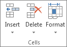
On the Home tab, in the Cells group, click Format.
-
Under Cell Size, do one of the following:
-
To fit all text in the cell, click AutoFit Column Width.
-
To specify a larger column width, click Column Width, and then type the width that you want in the Column width box.
-
Note: As an alternative to increasing the width of a column, you can change the format of that column or even an individual cell. For example, you could change the date format so that a date is displayed as only the month and day («mm/dd» format), such as 12/31, or represent a number in a Scientific (exponential) format, such as 4E+08.
Wrap text in a cell
You can display multiple lines of text inside a cell by wrapping the text. Wrapping text in a cell does not affect other cells.
-
Click the cell in which you want to wrap the text.
-
On the Home tab, in the Alignment group, click Wrap Text.
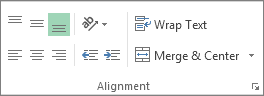
Note: If the text is a long word, the characters won’t wrap (the word won’t be split); instead, you can widen the column or decrease the font size to see all the text. If all the text is not visible after you wrap the text, you might have to adjust the height of the row. On the Home tab, in the Cells group, click Format, and then under Cell Size click AutoFit Row.
For more information on wrapping text, see the article Wrap text in a cell.
Change the format of a number
In Excel, the format of a cell is separate from the data that is stored in the cell. This display difference can have a significant effect when the data is numeric. For example, when a number that you enter is rounded, usually only the displayed number is rounded. Calculations use the actual number that is stored in the cell, not the formatted number that is displayed. Hence, calculations might appear inaccurate because of rounding in one or more cells.
After you type numbers in a cell, you can change the format in which they are displayed.
-
Click the cell that contains the numbers that you want to format.
-
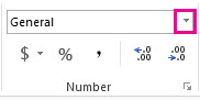
On the Home tab, in the Number group, click the arrow next to the Number Format box, and then click the format that you want.
To select a number format from the list of available formats, click More Number Formats, and then click the format that you want to use in the Category list.
Format a number as text
For numbers that should not be calculated in Excel, such as phone numbers, you can format them as text by applying the Text format to empty cells before typing the numbers.
-
Select an empty cell.
-
On the Home tab, in the Number group, click the arrow next to the Number Format box, and then click Text.
-
Type the numbers that you want in the formatted cell.
Numbers that you entered before you applied the Text format to the cells must be entered again in the formatted cells. To quickly reenter numbers as text, select each cell, press F2, and then press Enter.
Need more help?
You can always ask an expert in the Excel Tech Community or get support in the Answers community.
Need more help?
Want more options?
Explore subscription benefits, browse training courses, learn how to secure your device, and more.
Communities help you ask and answer questions, give feedback, and hear from experts with rich knowledge.
- Remove From My Forums
-
Question
-
Hi, My problem encountered is
— when i click on the excel’s cell, i’m unable to type in the word directly unless i double click on each of the cell only can type.
After tried to restart the excel, then it works.
May I know any cause on this or any solution for this?Because it keeps happening out of sudden and i have tried to reinstall and disable all the adds-on but still the same.
Anyone can help?!!
Answers
-
Have you checked if you disabled ‘allow editing directly in cells’?
1. Select File->Options->Advanced from the excel menu bar.
2. On Editing Options ,Ensure that the check box «Edit Directly in cell» is checked.-
Marked as answer by
Friday, November 8, 2013 1:58 AM
-
Marked as answer by
|
10-08-2017, 06:28 PM |
|||
|
|||
|
I can’t type numbers into excel cells — using 2013
|


|
10-09-2017, 12:30 AM |
||||
|
||||
|
Can you post the problem sheet here? It shouldn’t need any data on it, just say which cells you’re trying to use that don’t work.
|
|
10-09-2017, 06:23 AM |
|||
|
|||
|
Posting the offending spreadsheet I’ve attached the spreadsheet to this reply.
|
|
10-09-2017, 06:26 AM |
||||
|
||||
|
I can type freely anywhere in that sheet. Do you only have the problem with this one worksheet?
|
|
10-09-2017, 07:15 AM |
|||
|
|||
|
That is totally wierd I have had problems with other worksheets but it turned out those problems were caused by reference back to another worksheet. When I solved the reference problem it went away. This worksheet doesn’t refer to any other worksheet. With this worksheet try deleting some numbers and retype numbers back into those cells. Save the file, open it back up and again try typing in numbers. See if you can get the problem to surface after typing in numerous cells.
|
|
10-09-2017, 07:32 AM |
|||
|
|||
|
Just discovered something… I have been entering numbers from the number pad. I just double-clicked in a cell. It showed the cursor so I decided to type the number using the keys along the top of the keyboard. I checked the number pad and my NumLock wasn’t on. Sheesh!!! so many ways to stub a toe. Probably operator error, but I will post once more to inform whether or not this completely solved the problem. Thank you for looking at this.
|
Formatting Cell
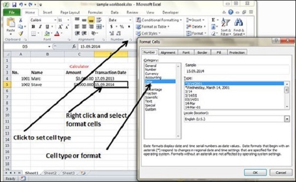
MS Excel Cell can hold different types of data like Numbers, Currency, Dates, etc. You can set the cell type in various ways as shown below −
- Right Click on the cell » Format cells » Number.
- Click on the Ribbon from the ribbon.
Various Cell Formats
Below are the various cell formats.
-
General − This is the default cell format of Cell.
-
Number − This displays cell as number with separator.
-
Currency − This displays cell as currency i.e. with currency sign.
-
Accounting − Similar to Currency, used for accounting purpose.
-
Date − Various date formats are available under this like 17-09-2013, 17th-Sep-2013, etc.
-
Time − Various Time formats are available under this, like 1.30PM, 13.30, etc.
-
Percentage − This displays cell as percentage with decimal places like 50.00%.
-
Fraction − This displays cell as fraction like 1/4, 1/2 etc.
-
Scientific − This displays cell as exponential like 5.6E+01.
-
Text − This displays cell as normal text.
-
Special − Special formats of cell like Zip code, Phone Number.
-
Custom − You can use custom format by using this.
This tutorial about cell format types in Excel is an essential part of your learning of Excel and will definitely do a lot of good to you in your future use of this software, as a lot of tasks in Excel sheets are based on cells format, as well as several errors are due to a bad implementation of it.
A good comprehension of the cell format types will build your knowledge on a solid basis to master Excel basics and will considerably save you time and effort when any related issue occurs.
A- Introduction
Excel software formats the cells depending on what type of information they contain.
To update the format of the highlighted cell, go to the “Home” tab of the ribbon and click, in the “Number” group of commands on the “Number Format” drop-down list.
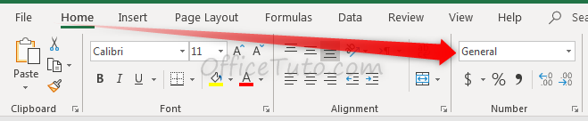
The drop-down list allows the selection to be changed.
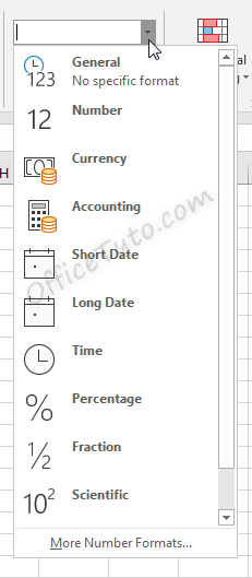
Cell formatting options in the “Number Format” drop-down list are:
- General
- Number
- Currency
- Accounting
- Short Date
- Long Date
- Time
- Percentage
- Fraction
- Scientific
- Text
- And the “More Number Formats” option.
Clicking the “More Number Formats” option brings up additional options for formatting cells, including the ability to do special and custom formatting options.
These options are discussed in detail in the below sections.
Cell format types in Excel are: General, Number, Currency, Accounting, Date, Time, Percentage, Fraction, Scientific, Text, Special (Zip Code, Zip Code + 4, Phone Number, Social Security Number), and Custom. You can get them from the “Number Format” drop-down list in the “Home” tab, or from the launcher arrow below it.
I will detail each one of them in the following sections:
1- General format
By default, cells are formatted as “General”, which could store any type of information. The General format means that no specific format is applied to the selected cell.
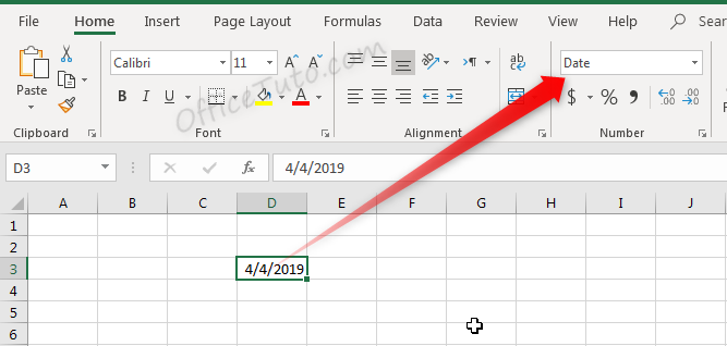
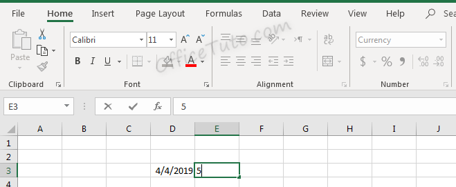
When information is typed into a cell, the cell format may change automatically. For example, if I enter “4/4/19” into a cell and press enter, then highlight the cell to view details about it, the cell format will be listed as “Date” instead of “General”.
Similarly, we can update a cell’s format before or after entering data to adjust the way the data appears. Changing the format of a cell to “Currency” will make it so information entered is displayed as a dollar amount.
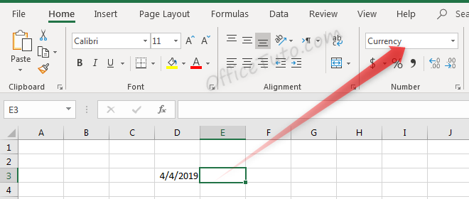
Typing a number into this cell and pressing enter will not just show that number, but will instead format it accordingly.
Before pressing enter, Excel shows the value which was typed: “4”.
After pressing enter, the value is updated based on the formatting type selected.
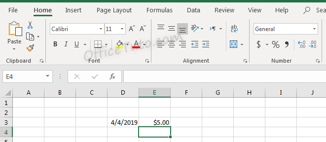
Don’t let the format type showed in the illustration at the drop-down list confusing you; it is reflecting the cell below (i.e. E4), since we validated by an Enter.
2- Number format
Cells formatted as numbers behave differently than general formatted cells. By default, when a number is entered, or when a cell is formatted as a number already, the alignment of the information within the cell will be on the right instead of on the left. This makes it easier to read a list of numbers such as the below.
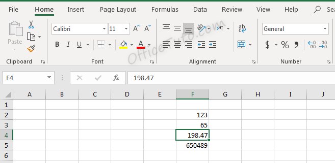
Note in the above screenshot that since we didn’t choose the “Number” format for our cells, they still have a “General” one. They are numbers for Excel (meaning, we can do calculations on them), but they didn’t have yet the number format and its formatting aspects:
You can set the formatting options for Excel numbers in the “Format Cells” dialog box.
To do that, select the cell or the range of cells you want to set the formatting options for their numbers, and go to the “Home” tab of the ribbon, then in the “Number” group of commands, click on the launcher of the dialog box (the arrow on the right-down side of the group).
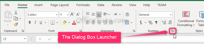
Excel opens the “Format Cells” dialog box in its “Number” tab. Click in the “Category” pane on “Number”.
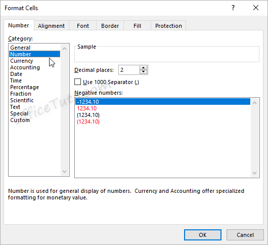
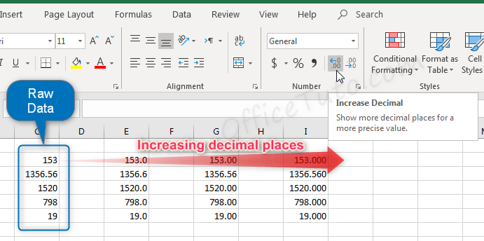
- In this dialog box, you can decide how many decimal places to display by updating options in the “Decimal places” field.
Note that this feature is also available in the “Home” tab of the ribbon where you can go to the “Number” group of commands and click the Increase Decimal ![]() or Decrease Decimal
or Decrease Decimal ![]() buttons.
buttons.
Here is the result of consecutive increasing of decimal places on our example of data (1 decimal; 2 decimals; and 3 decimals):
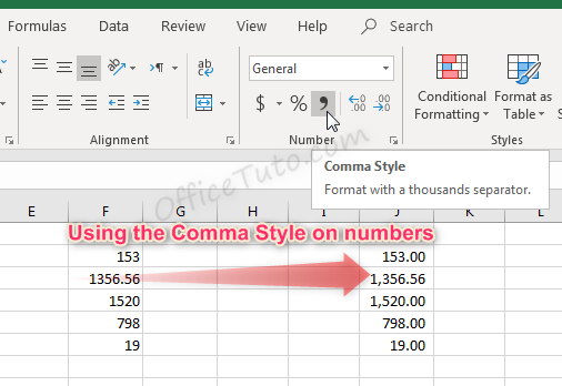
- You can also decide if commas should be shown in the display as a thousand separator, by updating the “Use 1000 Separator (,)” option in the “Format Cells” dialog box.
This feature is also available in the “Home” tab of the ribbon by clicking the “Comma Style” button ![]() in the “Number” group of commands.
in the “Number” group of commands.
Note that using the Comma Style button will automatically set the format to Accounting.
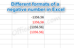
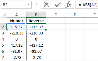
- Another option from the Format Cells dialog box is to decide how negative numbers should display by using the “Negative numbers” field.
There are four options for displaying negative
numbers.
- Display
negative numbers with a negative sign before the number. - Display
negative numbers in red. - Display
negative numbers in parentheses. - Display
negative numbers in red and in parentheses.
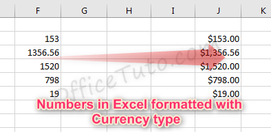
3- Currency format
Cells formatted as currency have a currency symbol such as a dollar sign $ immediately to the left of the number in the cell, and contain two numbers after the decimal by default.
The alignment of numbers in currency formatted cells will be on the right for readability.
Currency formatting options are similar to
number formatting options, apart from the currency symbol display.
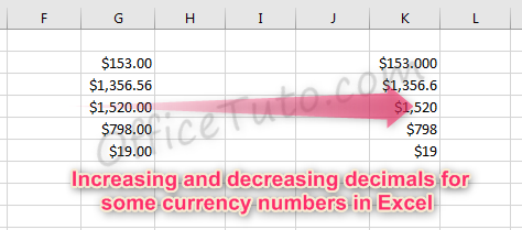
- As with regular number formatting, you can decide, in the “Format Cells” dialog box, how many decimal places to display by updating the field “Decimal places”.
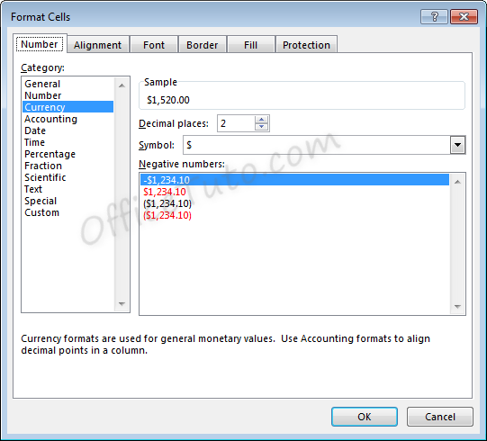
You can also find this feature in the “Home” tab of the ribbon, by going to the “Number” group of commands and clicking the Increase Decimal ![]() or Decrease Decimal
or Decrease Decimal ![]() .
.
- You can also decide what currency symbol should be shown in the display by updating the “Symbol” field in the “Format Cells” dialog box.
- As with regular number formatting, you can also decide how negative numbers should display by updating the “Negative numbers” field in the “Format Cells” dialog box.
There are four
options for displaying negative numbers.
- Display
negative numbers with a negative sign before the number. - Display
negative numbers in red. - Display
negative numbers in parentheses. - Display
negative numbers in red and in parentheses.
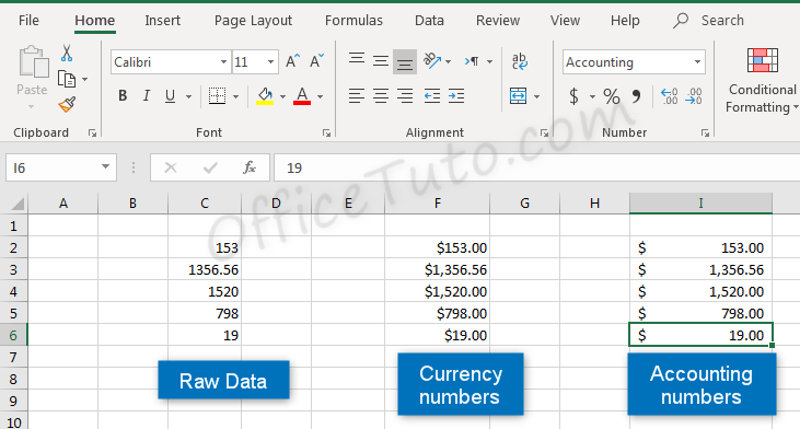
4- Accounting format
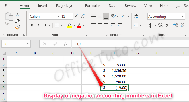
Like with the currency format, cells formatted as accounting have a currency symbol such as a dollar sign $; however, this symbol is to the far left of the cell, while the alignment of numbers in the cell is on the right. Accounting numbers contain two numbers after the decimal by default.
Clicking the “Accounting Number Format” button ![]() in the “Number” group of commands of the “Home” tab, will quickly format a cell or cells as Accounting.
in the “Number” group of commands of the “Home” tab, will quickly format a cell or cells as Accounting.
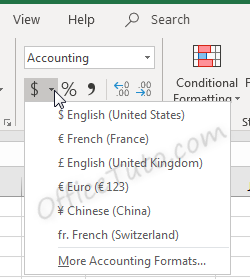
The down arrow to the right of the Accounting Number Format button allows selection between common symbols used for accounting, including English (dollar sign), English (pound), Euro, Chinese, and French symbols.
Accounting formatting options in the “Format Cells” dialog box (“Home” tab of the ribbon, in the “Number” group of commands, click on the launcher of the “Number Format” dialog box), are similar to number and currency formatting options.
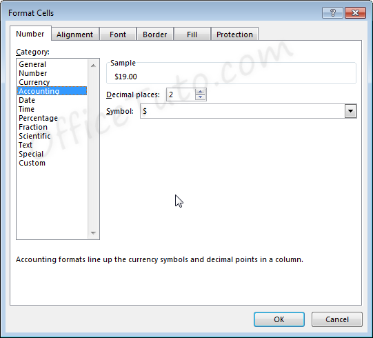
- You can decide how many decimal places to display by updating its option in the “Format Cells” dialog box.
As mentioned before in this tutorial, this feature is also available directly in the “Home” tab of the ribbon by clicking the Increase Decimal ![]() or Decrease Decimal
or Decrease Decimal ![]() buttons in the “Number” group of commands.
buttons in the “Number” group of commands.
- You can also decide in the “Format Cells” dialog box, what currency symbol should be shown in the display by using the “Symbol” drop-down list.
This dropdown gives a much broader list of options than the “Accounting Number Format” option in the “Home” tab of the ribbon.
Note that with the Accounting formatting option, negative numbers display in parentheses by default. There are not options to change this.
5- Date format
There are options for “Short Date” and “Long Date” in the “Number Format” dropdown list of the “Home” tab.
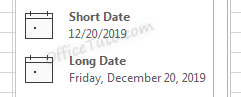
Short date shows the date with slashes separating month, day, and year. The order of the month and day may vary depending on your computer’s location settings.
Long date shows the date with the day of the week, month, day, and year separated by commas.
More options for formatting dates are available in the “Format Cells” dialog box (accessible by clicking in the “Number Format” dropdown list of the “Home” tab and choosing the “More Number Formats” option at the bottom).
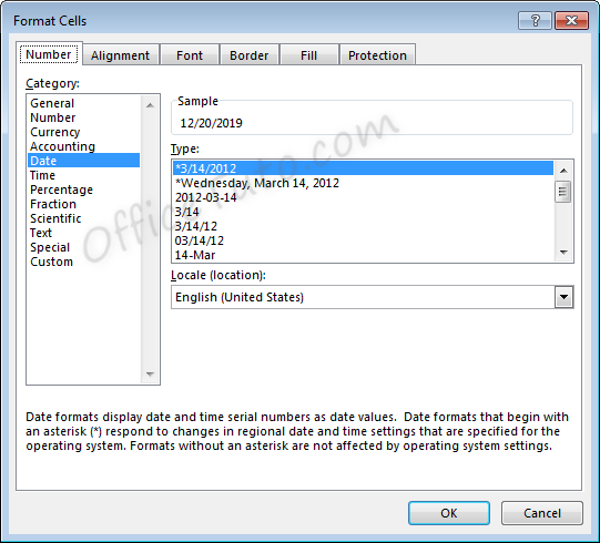
- You can choose from a long list of available date formats.
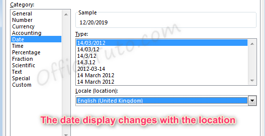
- You can update the location settings used for formatting the date. This will alter the list of format options in the above list and will adjust the display and potentially the order of the elements (day, month, year) within the date.
Note the below example when we switch from English (United States) format to English (United Kingdom) format.
6- Time format
Cells formatted as time display the time of
day. The default time display is based on your computer’s location settings.
Time formatting options are available in the “Format Cells” dialog box (accessible by choosing the “More Number Formats” option at the bottom of the “Number Format” dropdown list in the “Home” tab of the ribbon).
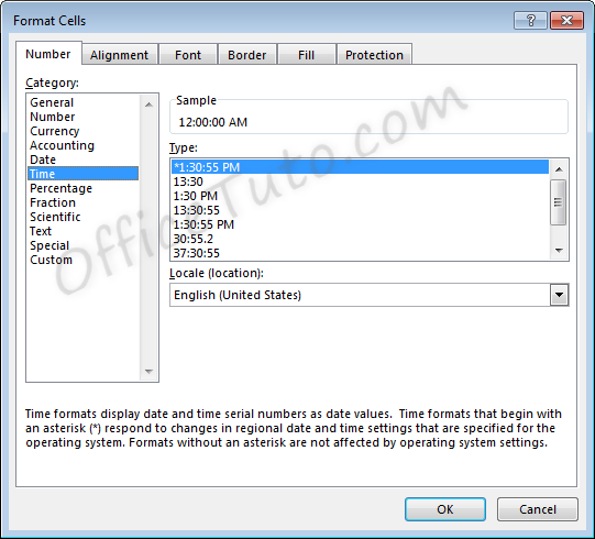
- You can choose from a long list of available time formats.
- You can update the location settings used for formatting the time. This will alter the list of format options in the above list and will adjust the display.
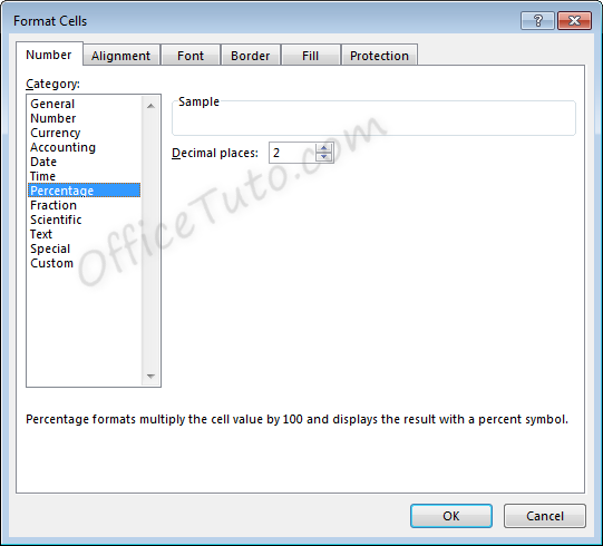
7- Percentage format
Cells formatted as percentage display a percent sign to the right of the number. You can change the format of a cell to a percentage using the “Number Format” dropdown list, or by clicking the “Percent Style” button ![]() . Both options are accessible from the “Home” tab of the ribbon, in the “Number” group of commands.
. Both options are accessible from the “Home” tab of the ribbon, in the “Number” group of commands.
Note that updating a number to a percentage
will expect that the number already contains the decimal. For example:
A cell containing the value 0.08, as a percentage, will show 8%.
A cell containing the value 8, as a percentage, will show 800%.
Percentage formatting options are available in the “Format Cells” dialog box, accessible by clicking on “More Number Formats” of the “Number Format” dropdown list in the “Home” tab of the ribbon.
8- Fraction format
Cells formatted as a fraction display with a slash
symbol separating the numerator and denominator.
Fraction formatting options are available in the “Format Cells” dialog box, accessible by clicking in the “Home” tab of the ribbon, on “More Number Formats” of the “Number Format” dropdown list.
- Note that
when selecting the format to use for a fraction, Excel will round to the
nearest fraction where the formatting criteria can be met.
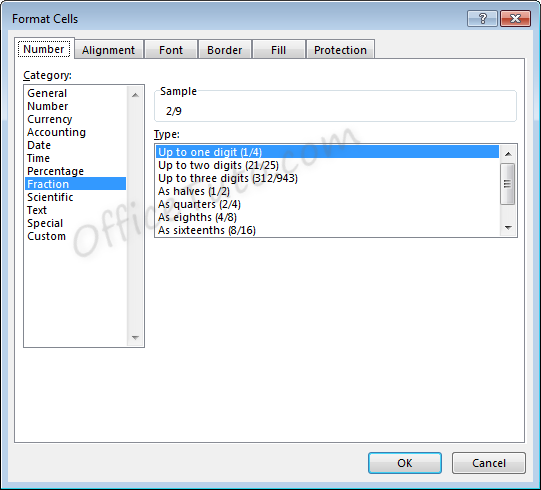
As an example, if the
formatting option selected is “Up to one digit”, entering a fraction with two
digits will cause rounding to occur. For example, with the setting of “Up to
one digit”,
If we enter a value of 7/16, the value displayed will be 4/9, as converting to 9ths was the option with only one digit which required the least amount of rounding.
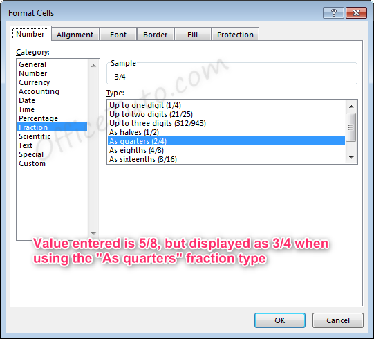
For another example, if the formatting option selected is “As quarters”, entering a fraction that cannot be expressed in quarters (divisible by four) will also cause rounding to occur.
If we enter a value of 5/8, the value displayed will be 3/4. Excel rounded up to 6/8, or 3/4, which was the closest option divisible by four.
- Also note
that for the formatting options with “Up to x digits”, Excel will always round
down to the lowest exact equivalent fraction when possible.
For example, if we enter a value of 2/4 with one of these formatting options active, the value displayed will be 1/2, as this is the mathematical equivalent. This behavior will not take place for formatting options “As…”, since these specifically determine what the denominator should be.
- Fractions listed as more than a whole (meaning the numerator is a higher number than the denominator), such as 7/4 will automatically be adjusted into a whole number and a fraction 13/4, where the fraction follows the formatting rules selected.
9- Scientific format
Scientific format, otherwise known as
Exponential Notation, allows very large and small numbers to be accurately
represented within a cell, even when the size of the cell cannot accommodate
the size of the numbers.
The way exponential notation works is to theoretically place a decimal in a spot that would make the number shorter, then describe where to move that decimal to return to the original number.
Examples with large numbers, where the decimal is moved to the left:
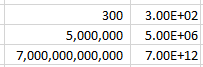
For the number 300 to be expressed in
exponential notation, Excel moves the decimal from after the whole number
300.00 to between the 3 and the 00. This is typed out as E+02 since the decimal
was moved two places to the left. The other examples are similar, where the
decimal was moved 6 and 12 places to the left.
Examples with small numbers, where the decimal is moved to the right:
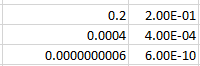
For the number 0.2 to be expressed in
exponential notation, Excel moves the decimal to create a whole number 2. This
is typed out as E-01 since the decimal was moved one place to the right. The
other examples are similar, where the decimal was moved 4 and 10 places to the
right.
Scientific formatting options are listed in the “Format Cells” dialog box, accessible by going to the “Home” tab of the ribbon, and clicking the “More Number Formats” option of the “Number Format” dropdown list.
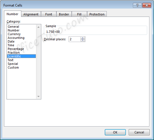
The only option available is to alter the
number of decimal places shown in the number prior to the scientific notation.
For example, for the value 11.43 formatted with the scientific format, if we change the Decimal places from 2 to 1, the display will change as follows.
Two decimals: 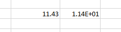
One decimal: 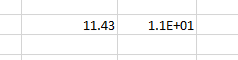
10- Text format
Cells can be formatted as Text through the
“Number Format” dropdown list, in the “Number” group of commands of the “Home”
tab.
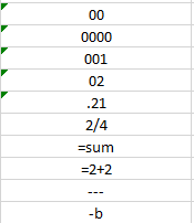
Using the Text format in Excel allows values to be entered as they are, without Excel changing them per the above formatting rules.
In general, when entering a text in a cell, you won’t need to set its type to “Text”, as the default format type “General” is sufficient in most cases.
This may be useful when you want to display numbers with leading zeros, want to have spaces before or after numbers or letters, or when you want to display symbols that Excel normally uses for formulas.
Below are examples of some fields formatted as Text.
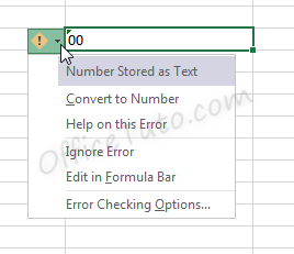
Note that when a number is formatted as Text, Excel will display a symbol showing that there could be a possible error ![]() .
.
Clicking the cell, then clicking the pop-up icon will show what the error may be and offer suggestions for resolution.
11- Special format
Special format offers four options in the “Format Cells” dialog box, accessible by going to the “Home” tab of the ribbon, and clicking the launcher arrow in the “Number” group of commands.
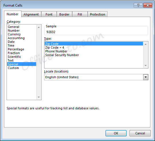
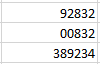
- Zip Code
When less than five numbers are entered in Zip
Code format, leading zeros will be added to bring the total to five numbers.
When more than five numbers are entered in Zip Code format, all numbers will be displayed, even though this does not meet the format criteria.
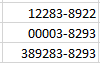
- Zip Code + 4
Zip Code + 4 format automatically creates a
dash symbol – before the last four numbers in the zip code.
When less than nine numbers are entered in Zip
Code + 4 format, leading zeros will be added to bring the total to nine
numbers.
When more than nine numbers are entered in Zip Code + 4 format, extra numbers are displayed prior to the dash symbol –.
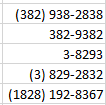
- Phone Number
Phone Number format automatically creates a
dash –
before the last four numbers in the phone number. This format also adds
parentheses ( ) around the area code when an area code is entered.
When less than the expected number of digits
are entered in Phone Number format, only the entered digits will be displayed,
starting from the end of the phone number, as shown on the third and fourth
lines, below.
When more than the expected number of digits
are entered in Phone Number format, extra numbers are displayed within the area
code parentheses.
Note that Phone Number format in Excel does not handle the number 1 before an area code. This entry would be treated like any other extra number.
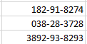
- Social Security Number
Social Security Number format automatically
creates a dash – before the last four numbers in the social security number
and a dash before the last six numbers in the social security number.
When less than nine numbers are entered in
Social Security Number format, leading zeros will be added to bring the total
to nine numbers.
When more than nine numbers are entered in Social Security Number format, extra numbers are displayed prior to the first dash –.
12- Custom format
Custom formats can be used or added through the
“Format Cells” dialog box, accessible from the “Number” group of commands in
the “Home” tab of the ribbon by clicking the “Number Format” launcher arrow.
This can be useful if the above formatting options do not work for your needs. Custom number formats can be created or updated by typing into the “Type” field of the “Format Cells” dialog box.
When creating a new custom format, be sure to use an existing custom format that you are okay with changing.
Custom number formats are separated, at
maximum, into four parts separated by semicolons ; .
- Part 1: How
to handle positive number values - Part 2: How
to handle negative number values - Part 3: How
to handle zero number values - Part 4: How
to handle text values
Note that if fewer parts are included in the custom format coding, Excel will determine how best to merge the above options: As an example, if two parts are listed, positive and zero values will be grouped.
Note that Excel may update the formatting of some fields to Custom automatically depending on what actions are taken on the field.
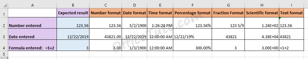
C- Common issues caused by wrong cell format types in Excel
1- Common issues due to wrong cell format types in Excel
The most common problems you may encounter with a wrong cell format type in Excel are of 3 types:
– Getting a wrong value.
– Getting an error.
– Formula displayed as-is and not calculated.
Let’s illustrate these 3 cases with some examples:
- Getting a wrong value
This may occur when you enter a value in an already formatted cell with an inappropriate format type, or when you apply a different format to a cell already containing a value.
The following table details some examples:
- Getting an error
This occurs when you enter a text preceded with a symbol of a dash, or plus, or equal, as an element of a list.
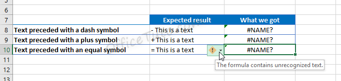
Excel wrongly interprets the text as a formula and show the error “The formula contains unrecognized text”.
- Formula displayed as-is and not calculated
In the following example, we tried to calculate the total of prices from cell B2 to B6 using the Excel SUM function, but Excel doesn’t calculate our formula and just displayed it as-is.
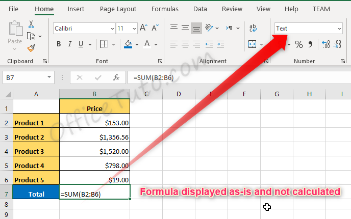
The source of the problem is that the result cell, B7, was previously formatted as text before entering the formula.
2- How to correct wrong cell format type issues in Excel
To correct cell format type issues in Excel, apply the right format in the “Number Format” drop-down list, and sometimes, you’ll also need to re-enter the content of the cell. For cells with formulas displayed as text, choose the “General” format, then double click in the cell and press Enter.

Jeff Golden is an experienced IT specialist and web publisher that has worked in the IT industry since 2010, with a focus on Office applications.
On this website, Jeff shares his insights and expertise on the different Office applications, especially Word and Excel.
In Excel, it is often necessary to use when calculating values that are tied to symbols, the sign of a number, and the type.
The following functions are used for this:
- CHAR;
- TYPE;
- SIGN.
CHAR function makes it possible to get a character with its given code. The function is used to convert the numeric character codes that are received from other computers into characters of the given computer.
TYPE function determines the data types of the cell, returning the corresponding number.
SIGN function returns the sign of a number and returns the value 1 if it is positive, 0 if it is 0, and -1 if it is negative.
Examples of using the CHAR, TYPE and SIGN functions in excel formulas
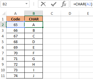
Example 1. Given a table with character codes: from 65 — to 74:
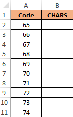
It is necessary with the help of the CHAR to display the characters that correspond to these codes.
To do this, we enter into the cell B2 the following formula:
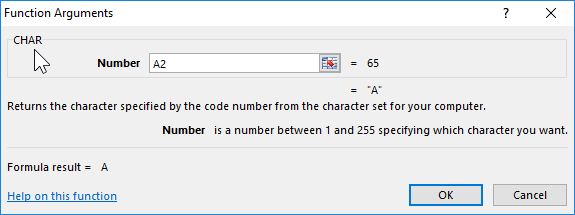
The function argument: Number is the character code.
As a result of the calculations we get:
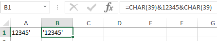
How to use the CHAR in formulas in practice? For example, we need to display a text string in single quotes. For Excel, a single quote as the first character is a special character that converts any cell value to a text data type. Therefore, in the cell itself, the single quote as the first character is not displayed:
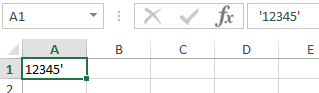
To solve this problem, we use the following formula with the function =CHAR(39)
It is also useful to use this function when you need to make a line break in an Excel cell as a formula. And for other similar tasks.
The value 39 in the function argument, you guessed it, is the character code of a single quote.
How to count the number of positive and negative numbers in Excel
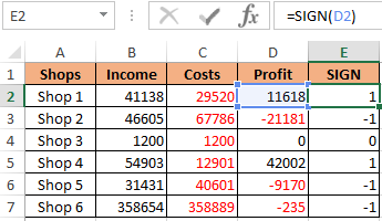
Example 2. The table contains 3 numbers. Calculate which character has each number: positive (+), negative (-) or 0.
Let’s enter the data in the table of the form:
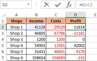
We introduce the formula in cell E2:
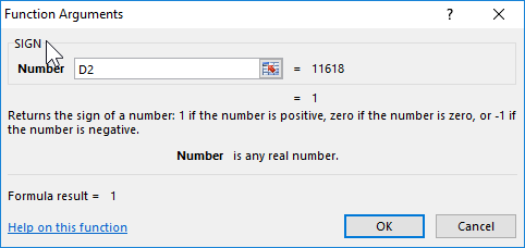
Argument: Number — any real numeric value.
By copying this formula down, we get:
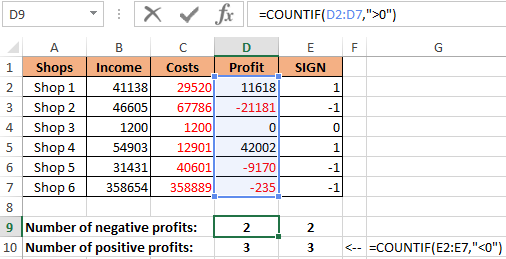
First, we calculate the number of negative and positive numbers in the columns «Profit» and «SIGN»:
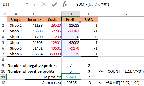
And now we summarize only positive or only negative numbers:
How to make a negative number positive and positive negative? It is very simple to multiply by -1:
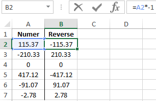
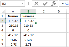
You can even simplify the formula, simply put a subtraction operator sign — minus, before the cell reference:
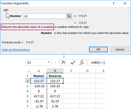
But what if you need to make a number with any sign positive? Then you should use the ABS function. This function returns any number by module:
Now it is not difficult to guess how to make any number with a negative minus sign:
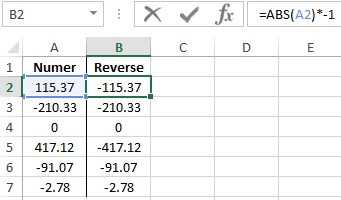
Or so:
Checking what types of cell input data in an Excel spreadsheet
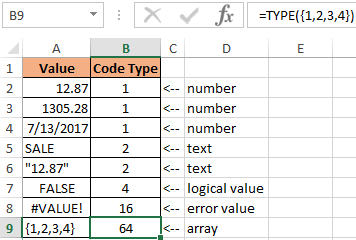
Example 3. Using the TYPE function, display the type of data that is entered in the table:
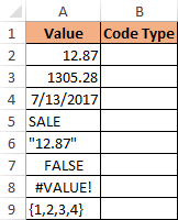
TYPE function returns the code of the data types that can be entered into an Excel cell:
| Data Value | Type Code |
| number | 1 |
| text | 2 |
| logical value | 4 |
| error value | 16 |
| array | 64 |
We introduce the formula for the calculation in cell B2:
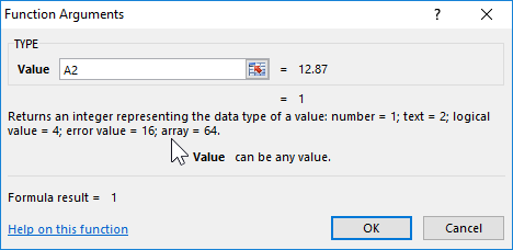
Argument: Value is any valid value.
As a result, we get:
Download examples functions CHAR SIGN TYPE in Excel
Thus, using the TYPE function, you can always check what the Excel cell actually contains. Note that the date is defined by the function as a number. For Excel, any date is a numeric value that corresponds to the number of days that have passed from January 01/01/1900, to the original date. Therefore, each date in Excel should be taken as a numeric data type displayed in the cell format — “Date”.
So, you have decided that time has come to become an Excel Master. Congratulations!
Before you start with Excel functions and tools, there are some basics that need to be covered first.
Let’s start our magical journey in Excel together! 🙂
A really quick intro to Excel
Excel is the world’s most popular spreadsheet software, developed by Microsoft.
Excel debuted on September 30, 1985, and since that day, kept evolving to meet the requirements of the spreadsheet community.
Most of the Excel versions require installation on your local computer. However, In recent years, Excel can be used online, via Excel Online!
And the best thing? Excel Online is absolutely free.
This website utilizes the technology of Excel Online to help you learn and practice Excel without the need have Excel installed on your computer. Thanks Microsoft! 🙂
So, let’s finish with the talking and start practicing!
Typing in Excel
Excel can be used for complex calculations, but you can always use it to type regular text, just like you’d do in Word or any other software.
All you have to do is select one of the cells and start typing…
You can start by typing your name, your favorite pet, your favorite movie and your lucky number 🙂
When you finish typing, hit the Enter key to exit the cell edit mode.
As you can see, you can type both text and numbers in Excel.
Did you notice that certain parts of the sheets changed after you typed your details? This was done using Excel formulas, which we will cover in the next tutorials 🙂
How does Excel work?
Let’s discuss some of the basic ideas in Excel:
- Excel Cell
- Excel Range
- Excel Worksheet
- Excel Workbook
1. Excel Cell
The Excel Cell is the smallest unit in Excel. The cell is used to store data.
In the previous example, we typed our names and favorite pets, movies and numbers in different Excel Cells.
Excel is comprised of rows and columns. The rows are represented as numbers, and the columns – as letters.
In order to reference a specific cell in Excel, we will type its column letter, followed by the row number.
So, A1 will be the first cell in your worksheet – It’s in the first column (A), and in the first row (1):

Ok, now let’s practice… Type your First Name in cell C3, and your Last Name in cell C4
2. Excel Range
The Excel Range is comprised of two or more adjacent cells. These cells can be in the same row, the same column, or even in multiple rows and columns!
Each range is represented by two cells – The top-left cell, and the bottom-right cell, separated with colons.
For example, Range A3:E7 consists of the following cells:

Now, it’s your time to play with Excel ranges!
3. Excel Worksheet
The Excel Worksheet is comprised of rows and columns.
The default Excel Worksheet contains 1,048,576 rows and 16,384 columns.
In the following example, we have 4 different worksheets:

Tip – We can quickly navigate between worksheets using the shortcut Ctrl+Page Up/Ctrl+Page Down. Click here for more useful Excel shortcuts!
4. Excel Workbook
The Excel file is also called Excel Workbook. It contains one or more worksheets.
The default Excel file type has an XLSX suffix.
Excel allows the user to use data from one worksheet in another worksheet in the same workbook. It also allows connecting between different workbooks.
Basic Calculations with Excel
OK, let’s start with the fun part!
We can perform calculations in Excel easily.
In order to start a calculation in a cell, we will type the = sign (equals), and then type our calculation.
These are the basic operators which can be used:
+ Add
– Substract
/ Divide
* (Asterisk) Multiply
^ Power
So, let’s say we want to find the result of 2+2:

Ok, now let’s practice!
Cell References
Okay, now that we know how to perform basic calculations, let’s learn how we can use cell references to make our calculations much quicker, and dynamic, as well!
If we type the = (equals) sign, followed by a reference to a cell (either by typing the cell name or clicking it), we can reference the data stored in that cell. We can also perform calculations using this way – Instead of manually typing the numbers, we can just reference the cells containing these numbers!
Let’s see how it works:

You can see in the example above that each time we change the data in the referenced cell – It is automatically reflected in the second cell!
Now, time to play with Excel:
Reusing cell references & using Partial and Absolute References
One of the advantages of using cell references in Excel is that we can reuse cell references in adjacent cells by copying the cell, or by dragging the cell to adjacent cells.
Let’s see how it works:

Sometimes, we would like that a certain reference will not move if we reuse the formula in other cells.
In such cases, we can use an Absolute Reference, by hitting the F4 button (or manually typing the $ signs before the column and/or row – not recommended) after typing the cell reference.
Let’s see this in action:

In certain cases, we might prefer using a Partial Reference rather than an Absolute Reference.
A Partial Reference allows us to keep the same reference only for a part of the cell – either the row or the column.
To use Partial Reference, just hit the F4 button until the deserved result is achieved.
Let’s see how we can do the entire Multiplication Table calculation, using only one formula!

Now you are all set to continue your Excel journey and learn how to use Excel functions and tools. Good luck! 🙂