
Overview of formulas in Excel
Get started on how to create formulas and use built-in functions to perform calculations and solve problems.

Important: The calculated results of formulas and some Excel worksheet functions may differ slightly between a Windows PC using x86 or x86-64 architecture and a Windows RT PC using ARM architecture. Learn more about the differences.
Important: In this article we discuss XLOOKUP and VLOOKUP, which are similar. Try using the new XLOOKUP function, an improved version of VLOOKUP that works in any direction and returns exact matches by default, making it easier and more convenient to use than its predecessor.
Create a formula that refers to values in other cells
-
Select a cell.
-
Type the equal sign =.
Note: Formulas in Excel always begin with the equal sign.
-
Select a cell or type its address in the selected cell.

-
Enter an operator. For example, – for subtraction.
-
Select the next cell, or type its address in the selected cell.
-
Press Enter. The result of the calculation appears in the cell with the formula.


See a formula
-
When a formula is entered into a cell, it also appears in the Formula bar.
-
To see a formula, select a cell, and it will appear in the formula bar.


Enter a formula that contains a built-in function
-
Select an empty cell.
-
Type an equal sign = and then type a function. For example, =SUM for getting the total sales.
-
Type an opening parenthesis (.
-
Select the range of cells, and then type a closing parenthesis).
-
Press Enter to get the result.

Download our Formulas tutorial workbook
We’ve put together a Get started with Formulas workbook that you can download. If you’re new to Excel, or even if you have some experience with it, you can walk through Excel’s most common formulas in this tour. With real-world examples and helpful visuals, you’ll be able to Sum, Count, Average, and Vlookup like a pro.
Formulas in-depth
You can browse through the individual sections below to learn more about specific formula elements.
A formula can also contain any or all of the following: functions, references, operators, and constants.
Parts of a formula

1. Functions: The PI() function returns the value of pi: 3.142…
2. References: A2 returns the value in cell A2.
3. Constants: Numbers or text values entered directly into a formula, such as 2.
4. Operators: The ^ (caret) operator raises a number to a power, and the * (asterisk) operator multiplies numbers.
A constant is a value that is not calculated; it always stays the same. For example, the date 10/9/2008, the number 210, and the text «Quarterly Earnings» are all constants. An expression or a value resulting from an expression is not a constant. If you use constants in a formula instead of references to cells (for example, =30+70+110), the result changes only if you modify the formula. In general, it’s best to place constants in individual cells where they can be easily changed if needed, then reference those cells in formulas.
A reference identifies a cell or a range of cells on a worksheet, and tells Excel where to look for the values or data you want to use in a formula. You can use references to use data contained in different parts of a worksheet in one formula or use the value from one cell in several formulas. You can also refer to cells on other sheets in the same workbook, and to other workbooks. References to cells in other workbooks are called links or external references.
-
The A1 reference style
By default, Excel uses the A1 reference style, which refers to columns with letters (A through XFD, for a total of 16,384 columns) and refers to rows with numbers (1 through 1,048,576). These letters and numbers are called row and column headings. To refer to a cell, enter the column letter followed by the row number. For example, B2 refers to the cell at the intersection of column B and row 2.
To refer to
Use
The cell in column A and row 10
A10
The range of cells in column A and rows 10 through 20
A10:A20
The range of cells in row 15 and columns B through E
B15:E15
All cells in row 5
5:5
All cells in rows 5 through 10
5:10
All cells in column H
H:H
All cells in columns H through J
H:J
The range of cells in columns A through E and rows 10 through 20
A10:E20
-
Making a reference to a cell or a range of cells on another worksheet in the same workbook
In the following example, the AVERAGE function calculates the average value for the range B1:B10 on the worksheet named Marketing in the same workbook.
1. Refers to the worksheet named Marketing
2. Refers to the range of cells from B1 to B10
3. The exclamation point (!) Separates the worksheet reference from the cell range reference
Note: If the referenced worksheet has spaces or numbers in it, then you need to add apostrophes (‘) before and after the worksheet name, like =’123′!A1 or =’January Revenue’!A1.
-
The difference between absolute, relative and mixed references
-
Relative references A relative cell reference in a formula, such as A1, is based on the relative position of the cell that contains the formula and the cell the reference refers to. If the position of the cell that contains the formula changes, the reference is changed. If you copy or fill the formula across rows or down columns, the reference automatically adjusts. By default, new formulas use relative references. For example, if you copy or fill a relative reference in cell B2 to cell B3, it automatically adjusts from =A1 to =A2.
Copied formula with relative reference
-
Absolute references An absolute cell reference in a formula, such as $A$1, always refer to a cell in a specific location. If the position of the cell that contains the formula changes, the absolute reference remains the same. If you copy or fill the formula across rows or down columns, the absolute reference does not adjust. By default, new formulas use relative references, so you may need to switch them to absolute references. For example, if you copy or fill an absolute reference in cell B2 to cell B3, it stays the same in both cells: =$A$1.
Copied formula with absolute reference
-
Mixed references A mixed reference has either an absolute column and relative row, or absolute row and relative column. An absolute column reference takes the form $A1, $B1, and so on. An absolute row reference takes the form A$1, B$1, and so on. If the position of the cell that contains the formula changes, the relative reference is changed, and the absolute reference does not change. If you copy or fill the formula across rows or down columns, the relative reference automatically adjusts, and the absolute reference does not adjust. For example, if you copy or fill a mixed reference from cell A2 to B3, it adjusts from =A$1 to =B$1.
Copied formula with mixed reference
-
-
The 3-D reference style
Conveniently referencing multiple worksheets If you want to analyze data in the same cell or range of cells on multiple worksheets within a workbook, use a 3-D reference. A 3-D reference includes the cell or range reference, preceded by a range of worksheet names. Excel uses any worksheets stored between the starting and ending names of the reference. For example, =SUM(Sheet2:Sheet13!B5) adds all the values contained in cell B5 on all the worksheets between and including Sheet 2 and Sheet 13.
-
You can use 3-D references to refer to cells on other sheets, to define names, and to create formulas by using the following functions: SUM, AVERAGE, AVERAGEA, COUNT, COUNTA, MAX, MAXA, MIN, MINA, PRODUCT, STDEV.P, STDEV.S, STDEVA, STDEVPA, VAR.P, VAR.S, VARA, and VARPA.
-
3-D references cannot be used in array formulas.
-
3-D references cannot be used with the intersection operator (a single space) or in formulas that use implicit intersection.
What occurs when you move, copy, insert, or delete worksheets The following examples explain what happens when you move, copy, insert, or delete worksheets that are included in a 3-D reference. The examples use the formula =SUM(Sheet2:Sheet6!A2:A5) to add cells A2 through A5 on worksheets 2 through 6.
-
Insert or copy If you insert or copy sheets between Sheet2 and Sheet6 (the endpoints in this example), Excel includes all values in cells A2 through A5 from the added sheets in the calculations.
-
Delete If you delete sheets between Sheet2 and Sheet6, Excel removes their values from the calculation.
-
Move If you move sheets from between Sheet2 and Sheet6 to a location outside the referenced sheet range, Excel removes their values from the calculation.
-
Move an endpoint If you move Sheet2 or Sheet6 to another location in the same workbook, Excel adjusts the calculation to accommodate the new range of sheets between them.
-
Delete an endpoint If you delete Sheet2 or Sheet6, Excel adjusts the calculation to accommodate the range of sheets between them.
-
-
The R1C1 reference style
You can also use a reference style where both the rows and the columns on the worksheet are numbered. The R1C1 reference style is useful for computing row and column positions in macros. In the R1C1 style, Excel indicates the location of a cell with an «R» followed by a row number and a «C» followed by a column number.
Reference
Meaning
R[-2]C
A relative reference to the cell two rows up and in the same column
R[2]C[2]
A relative reference to the cell two rows down and two columns to the right
R2C2
An absolute reference to the cell in the second row and in the second column
R[-1]
A relative reference to the entire row above the active cell
R
An absolute reference to the current row
When you record a macro, Excel records some commands by using the R1C1 reference style. For example, if you record a command, such as clicking the AutoSum button to insert a formula that adds a range of cells, Excel records the formula by using R1C1 style, not A1 style, references.
You can turn the R1C1 reference style on or off by setting or clearing the R1C1 reference style check box under the Working with formulas section in the Formulas category of the Options dialog box. To display this dialog box, click the File tab.
Top of Page


Need more help?
You can always ask an expert in the Excel Tech Community or get support in the Answers community.
See Also
Switch between relative, absolute and mixed references for functions
Using calculation operators in Excel formulas
The order in which Excel performs operations in formulas
Using functions and nested functions in Excel formulas
Define and use names in formulas
Guidelines and examples of array formulas
Delete or remove a formula
How to avoid broken formulas
Find and correct errors in formulas
Excel keyboard shortcuts and function keys
Excel functions (by category)
Need more help?
Want more options?
Explore subscription benefits, browse training courses, learn how to secure your device, and more.
Communities help you ask and answer questions, give feedback, and hear from experts with rich knowledge.
![]()
Download Article
![]()
Download Article
Microsoft Excel’s power is in its ability to calculate and display results from data entered into its cells. To calculate anything in Excel, you need to enter formulas into its cells. Formulas can be simple arithmetical formulas or complicated formulas involving conditional statements and nested functions. All Excel formulas use a basic syntax, which is described in the steps below.
-
1
Begin every formula with an equal sign (=). The equal sign tells Excel that the string of characters you’re entering into a cell is a mathematical formula. If you forget the equal sign, Excel will treat the entry as a character string.
-
2
Use coordinate references for cells that contain the values used in your formula. While you can include numeric constants in your formulas, in most cases you’ll use values entered in other cells (or the results of other formulas displayed in those cells) in your formulas. You refer to those cells with a coordinate reference of the row and column the cell is in. There are several formats:
- The most common coordinate reference is to use the letter or letters representing the column followed by the number of the row the cell is in: A1 refers to the cell in Column A, Row 1. If you add rows above the referenced cell or columns above the referenced cell, the cell’s reference will change to reflect its new position; adding a row above Cell A1 and a column to its left will change its reference to B2 in any formula the cell is referenced in.
- A variation of this reference is to make row or column references absolute by preceding them with a dollar sign ($). While the reference name for Cell A1 will change if a row is added above or a column is added in front of it, Cell $A$1 will always refer to the cell in the upper left corner of the spreadsheet; thus, in a formula, Cell $A$1, could have a different, or even invalid, value in the formula if rows or columns are inserted in the spreadsheet. (You can make only the row or column cell reference absolute, if you wish.)
- Another way to reference cells is numerically, in the format RxCy, where «R» indicates «row,» «C» indicates «column,» and «x» and «y» are the row and column numbers. Cell R5C4 in this format would be the same as Cell $D$5 in absolute column, row reference format. Putting either number after the «R» or the «C» makes that reference relative to the upper left corner of the spreadsheet page.
- If you use only an equal sign and a single cell reference in your formula, you copy the value from the other cell into your new cell. Entering the formula «=A2» in Cell B3 will copy the value entered into Cell A2 into Cell B3. To copy the value from a cell in one spreadsheet page to a cell on a different page, include the page name, followed by an exclamation point (!). Entering «=Sheet1!B6» in Cell F7 on Sheet2 of the spreadsheet displays the value of Cell B6 on Sheet1 in Cell F7 on Sheet2.
Advertisement
-
3
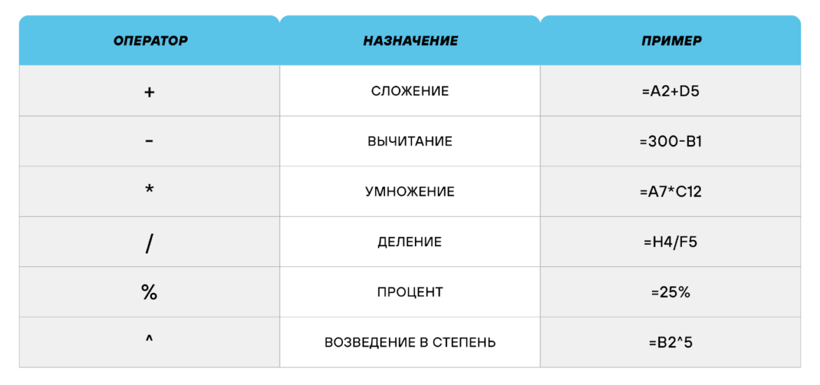
Use arithmetic operators for basic calculations. Microsoft Excel can perform all of the basic arithmetic operations �- addition, subtraction, multiplication, and division -� as well as exponentiation. Some operations use different symbols than are used when writing equations by hand. A list of operators is given below, in the order in which Excel processes arithmetic operations:
- Negation: A minus sign (-). This operation returns the additive inverse of the number represented by the numeric constant or cell reference following the minus sign. (The additive inverse is the value added to a number to produce a value of zero; it’s the same as multiplying the number by -1.)
- Percentage: The percent sign (%). This operation returns the decimal equivalent of the percentage of the numeric constant in front of the number.
- Exponentiation: A caret (^). This operation raises the number represented by the cell reference or constant in front of the caret to the power of the number after the caret.
- Multiplication: An asterisk (*). An asterisk is used for multiplication to avoid confusion with the letter «x.»
- Division: A forward slash (/). Multiplication and division have equal precedence and are performed from left to right.
- Addition: A plus sign (+).
- Subtraction: A minus sign (-). Addition and subtraction have equal precedence and are performed from left to right.
-
4
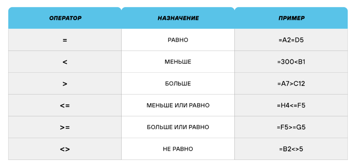
Use comparison operators to compare the values in cells. You’ll use comparison operators most often in formulas with the IF function. You place a cell reference, numeric constant, or function that returns a numeric value on either side of the comparison operator. The comparison operators are listed below:
- Equals: An equal sign (=).
- Is not equal to (<>).
- Less than (<).
- Less than or equal to (<=).
- Greater than (>).
- Greater than or equal to (>=).
-
5
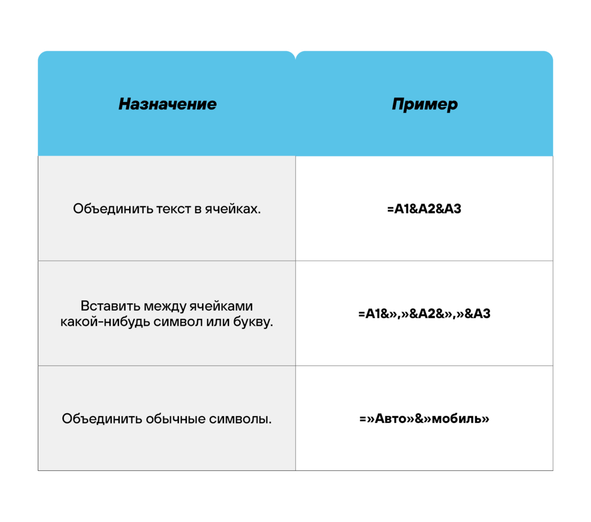
Use an ampersand (&) to join text strings together. The joining of text strings into a single string is called concatenation, and the ampersand is known as a text operator when used to join strings together in Excel formulas. You can use it with text strings or cell references or both; entering «=A1&B2» in Cell C3 will yield «BATMAN» when «BAT» is entered in Cell A1 and «MAN» is entered in Cell B2.
-
6
Use reference operators when working with ranges of cells. You’ll use ranges of cells most often with Excel functions such as SUM, which finds the sum of a range of cells. Excel uses 3 reference operators:
- Range operator: a colon (:). The range operator refers to all cells in a range beginning with the referenced cell in front of the colon and ending with the referenced cell after the colon. All the cells are usually in the same row or column; «=SUM(B6:B12)» displays the result of adding the column of cells from B6 through B12, while «=AVERAGE(B6:F6)» displays the average of the numbers in the row of cells from B6 through F6.
- Union operator: a comma (,). The union operator includes both the cells or ranges of cells named before the comma and those after it; «=SUM(B6:B12, C6:C12)» adds together the cells from B6 through B12 and C6 through C12.
- Intersection operator: a space ( ). The intersection operator identifies cells common to 2 or more ranges; listing the cell ranges «=B5:D5 C4:C6» yields the value in the cell C5, which is common to both ranges.
-
7
Use parentheses to identify the arguments of functions and to override the order of operations. Parentheses serve 2 functions in Excel, to identify the arguments of functions and to specify a different order of operations than the normal order.
- Functions are pre-defined formulas. Some, such as SIN, COS, or TAN, take a single argument, while other functions, such as IF, SUM, or AVERAGE, may take multiple arguments. Multiple arguments within a function are separated by commas, as in «=IF (A4 >=0, «POSITIVE,» «NEGATIVE»)» for the IF function. Functions may be nested within other functions, up to 64 levels deep.
- In mathematical operation formulas, operations within parentheses are performed before those outside it; in «=A4+B4*C4,» B4 is multiplied by C4 before A4 is added to the result, but in «=(A4+B4)*C4,» A4 and B4 are added together first, then the result is multiplied by C4. Parentheses in operations may be nested inside each other; the operation in the innermost set of parentheses will be performed first.
- Whether nesting parentheses in mathematical operations or in nested functions, always be sure to have as many close parentheses in your formula as you do open parentheses, or you’ll receive an error message.


Advertisement
-
1
Select the cell you want to enter the formula in.
-
2
Type an equal sign the cell or in the formula bar. The formula bar is located above the rows and columns of cells and beneath the menu bar or ribbon.
-
3
Type an open parenthesis if necessary. Depending on the structure of your formula, you may need to type several open parentheses.
-
4
Create a cell reference. You can do this in 1 of several ways: Type the cell reference manually.Select a cell or range of cells in the current page of the spreadsheet.Select a cell or range of cells in another page of the spreadsheet.Select a cell or range of cells on a page of a different spreadsheet.
-
5
Enter a mathematical, comparison, text, or reference operator if desired. For most formulas, you’ll use a mathematical operator or 1 of the reference operators.
-
6
Repeat the previous 3 steps as necessary to build your formula.
-
7
Type a close parenthesis for each open parenthesis in your formula.
-
8
Press «Enter» when your formula is the way you want it to be.


Advertisement
Add New Question
-
Question
What is the name of «;»?

It is called a semicolon, which can be used in programming languages to separate the statements or print variables by using one output statement.
-
Question
How do I subtract one cell from another in Excel?
If you want to subtract cell A1 from cell B1, in cell C1 you would type «=A1-B1» and hit enter. You can also use the autosum feature in the far right of the header.
-
Question
How do I type the symbols that are used in Excel?
You click Shift and the number/letter you see the symbol on (for example, if you want the multiplication symbol * you hit Shift+8) when using a keyboard. On a phone you have to switch the keyboard to the special characters one and find the symbol you want.
See more answers
Ask a Question
200 characters left
Include your email address to get a message when this question is answered.
Submit
Advertisement
-
When you first start working with complex formulas, it may be helpful to write the formula out on paper before entering it into Excel. If the formula looks too complex to enter into a single cell, you can break it down into several parts and enter the parts into several cells, and use a simpler formula in another cell to combine the results of the individual formula parts together.
-
Microsoft Excel offers assistance in typing formulas with Formula AutoComplete, a dynamic list of functions, arguments, or other possibilities that appears after you type the equal sign and the first few characters of your formula. Press your «Tab» key or double-click an item in the dynamic list to insert it in your formula; if the item is a function, you will then be prompted to enter its arguments. You can turn this feature on or off by selecting «Formulas» on the «Excel Options» dialog and checking or unchecking the «Formula AutoComplete» box. (You access this dialog by selecting «Options» from the «Tools» menu in Excel 2003, from the «Excel Options» button on the «File» button menu in Excel 2007, and by selecting «Options» on the «File» tab menu in Excel 2010.)
-
When renaming the sheets in a multi-page spreadsheet, make it a practice not to use any spaces in the new sheet name. Excel won’t recognize naked spaces in sheet names in formula references. (You can also get around this problem by substituting an underscore for the space in the sheet name when using it in a formula.)
Thanks for submitting a tip for review!
Advertisement
-
Don’t include formatting such as commas or dollar signs in numbers when entering them in formulas because Excel recognizes commas as argument separators and union operators and dollar signs as absolute reference indicators.
Advertisement
About This Article
Thanks to all authors for creating a page that has been read 302,610 times.
Is this article up to date?
Самая популярная программа для работы с электронными таблицами «Microsoft Excel» упростила жизнь многим пользователям, позволив производить любые расчеты с помощью формул. Она способна автоматизировать даже самые сложные вычисления, но для этого нужно знать принципы работы с формулами. Мы подготовили самую подробную инструкцию по работе с Эксель. Не забудьте сохранить в закладки 😉
Содержание
-
Кому важно знать формулы Excel и где выучить основы.
-
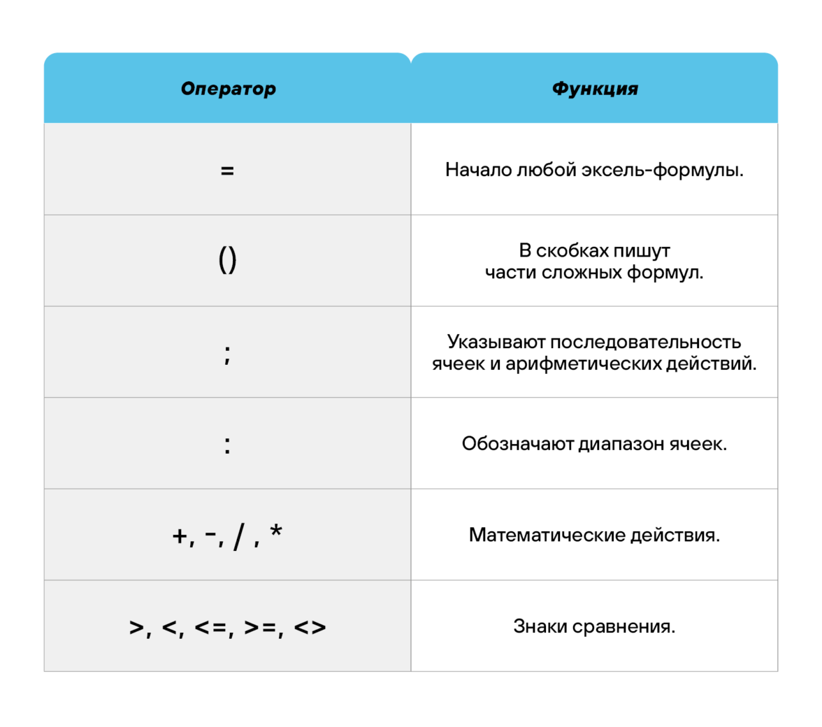
Элементы, из которых состоит формула в Excel.
-
Основные виды.
-
Примеры работ, которые можно выполнять с формулами.
-
22 формулы в Excel, которые облегчат жизнь.
-
Использование операторов.
-
Использование ссылок.
-
Использование имён.
-
Использование функций.
-
Операции с формулами.
-
Как в формуле указать постоянную ячейку.
-
Как поставить «плюс», «равно» без формулы.
-
Самые распространенные ошибки при составлении формул в редакторе Excel.
-
Коды ошибок при работе с формулами.
-
Отличие в версиях MS Excel.
-
Заключение.
Кому важно знать формулы Excel и где изучить основы
Excel — эффективный помощник бухгалтеров и финансистов, владельцев малого бизнеса и даже студентов. Менеджеры ведут базы клиентов, а маркетологи считают в таблицах медиапланы. Аналитики с помощью эксель формул обрабатывают большие объемы данных и строят гипотезы.
Эксель довольно сложная программа, но простые функции и базовые формулы можно освоить достаточно быстро по статьям и видео-урокам. Однако, если ваша профессиональная деятельность подразумевает работу с большим объемом данных и требует глубокого изучения возможностей Excel — стоит пройти специальные курсы, например тут или тут.
Элементы, из которых состоит формула в Excel
Формулы эксель: основные виды
Формулы в Excel бывают простыми, сложными и комбинированными. В таблицах их можно писать как самостоятельно, так и с помощью интегрированных программных функций.
Простые
Позволяют совершить одно простое действие: сложить, вычесть, разделить или умножить. Самой простой является формула=СУММ.
Например:
=СУММ (A1; B1) — это сумма значений двух соседних ячеек.
=СУММ (С1; М1; Р1) — сумма конкретных ячеек.
=СУММ (В1: В10) — сумма значений в указанном диапазоне.
Сложные
Это многосоставные формулы для более продвинутых пользователей. В данную категорию входят ЕСЛИ, СУММЕСЛИ, СУММЕСЛИМН. О них подробно расскажем ниже.
Комбинированные
Эксель позволяет комбинировать несколько функций: сложение + умножение, сравнение + умножение. Это удобно, когда, например, нужно вычислить сумму двух чисел, и, если результат будет больше 100, его нужно умножить на 3, а если меньше — на 6.
Выглядит формула так ↓
=ЕСЛИ (СУММ (A1; B1)<100; СУММ (A1; B1)*3;(СУММ (A1; B1)*6))
Встроенные
Новичкам удобнее пользоваться готовыми, встроенными в программу формулами вместо того, чтобы писать их вручную. Чтобы найти нужную формулу:
-
кликните по нужной ячейке таблицы;
-
нажмите одновременно Shift + F3;
-
выберите из предложенного перечня нужную формулу;
-
в окошко «Аргументы функций» внесите свои данные.
Примеры работ, которые можно выполнять с формулами
Разберем основные действия, которые можно совершить, используя формулы в таблицах Эксель и рассмотрим полезные «фишки» для упрощения работы.
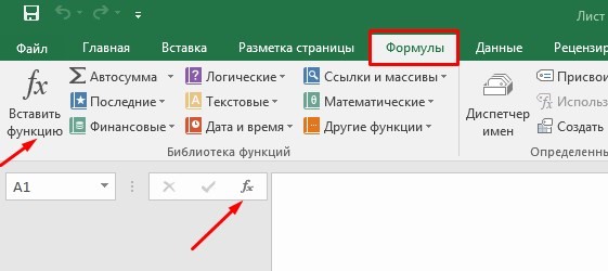
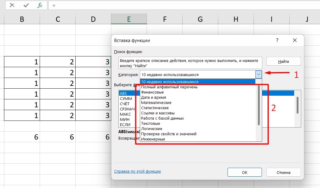
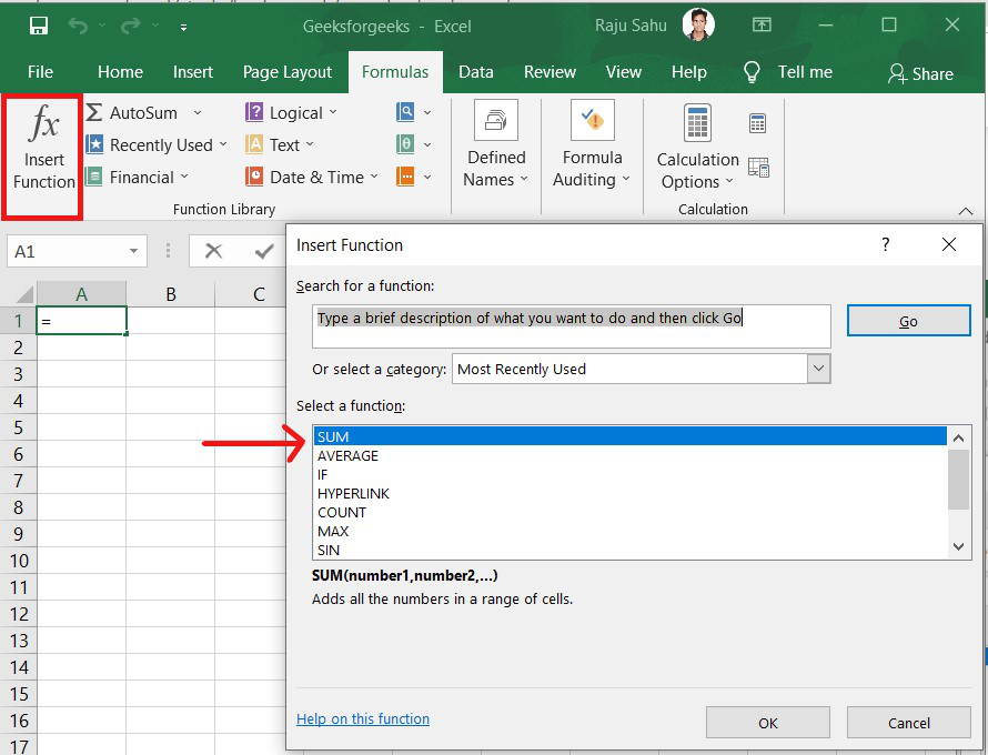
Поиск перечня доступных функций
Перейдите в закладку «Формулы» / «Вставить функцию». Или сразу нажмите на кнопочку «Fx».
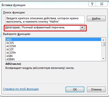
Выберите в категории «Полный алфавитный перечень», после чего в списке отобразятся все доступные эксель-формулы.
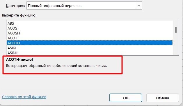
Выберите любую формулу и прочитайте ее описание. А если хотите изучить ее более детально, нажмите на «Справку» ниже.
Вставка функции в таблицу
Вы можете сами писать функции в Excel вручную после «=», или использовать меню, описанное выше. Например, выбрав СУММ, появится окошко, где нужно ввести аргументы (кликнуть по клеткам, значения которых собираетесь складывать):
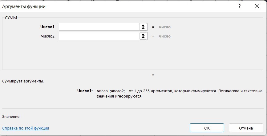
После этого в таблице появится формула в стандартном виде. Ее можно редактировать при необходимости.
Использование математических операций
Начинайте с «=» в ячейке и применяйте для вычислений любые стандартные знаки «*», «/», «^» и т.д. Можно написать номер ячейки самостоятельно или кликнуть по ней левой кнопкой мышки. Например: =В2*М2. После нажатия Enter появится произведение двух ячеек.
Растягивание функций и обозначение константы
Введите функцию =В2*C2, получите результат, а затем зажмите правый нижний уголок ячейки и протащите вниз. Формула растянется на весь выбранный диапазон и автоматически посчитает значения для всех строк от B3*C3 до B13*C13.
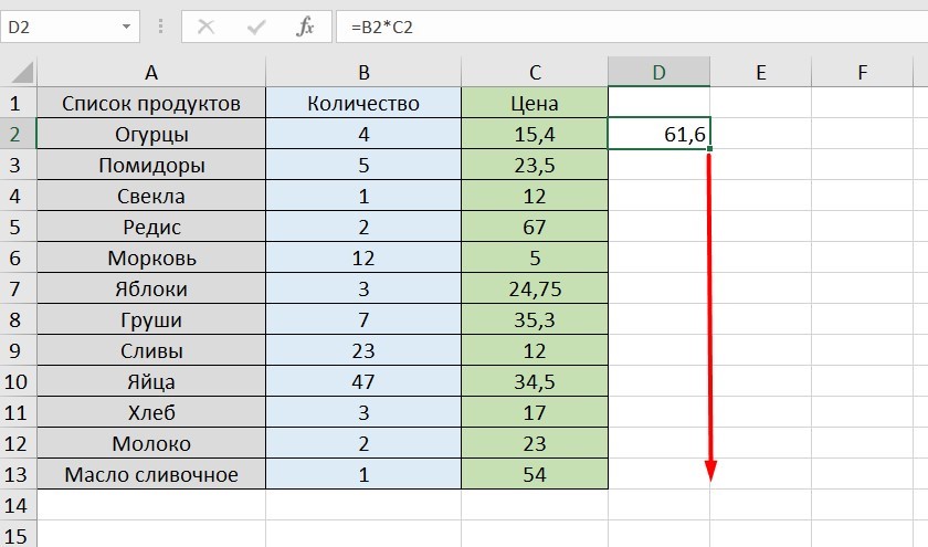
Чтобы обозначить константу (зафиксировать конкретную ячейку/строку/столбец), нужно поставить «$» перед буквой и цифрой ячейки.
Например: =В2*$С$2. Когда вы растяните функцию, константа или $С$2 так и останется неизменяемой, а вот первый аргумент будет меняться.
Подсказка:
-
$С$2 — не меняются столбец и строка.
-
B$2 — не меняется строка 2.
-
$B2 — константой остается только столбец В.
22 формулы в Эксель, которые облегчат жизнь
Собрали самые полезные формулы, которые наверняка пригодятся в работе.
МАКС
=МАКС (число1; [число2];…)
Показывает наибольшее число в выбранном диапазоне или перечне ячейках.
МИН
=МИН (число1; [число2];…)
Показывает самое маленькое число в выбранном диапазоне или перечне ячеек.
СРЗНАЧ
=СРЗНАЧ (число1; [число2];…)
Считает среднее арифметическое всех чисел в диапазоне или в выбранных ячейках. Все значения суммируются, а сумма делится на их количество.
СУММ
=СУММ (число1; [число2];…)
Одна из наиболее популярных и часто используемых функций в таблицах Эксель. Считает сумму чисел всех указанных ячеек или диапазона.
ЕСЛИ
=ЕСЛИ (лог_выражение; значение_если_истина; [значение_если_ложь])
Сложная формула, которая позволяет сравнивать данные.
Например:
=ЕСЛИ (В1>10;”больше 10″;»меньше или равно 10″)
В1 — ячейка с данными;
>10 — логическое выражение;
больше 10 — правда;
меньше или равно 10 — ложное значение (если его не указывать, появится слово ЛОЖЬ).
СУММЕСЛИ
=СУММЕСЛИ (диапазон; условие; [диапазон_суммирования]).
Формула суммирует числа только, если они отвечают критерию.
Например:
=СУММЕСЛИ (С2: С6;»>20″)
С2: С6 — диапазон ячеек;
>20 —значит, что числа меньше 20 не будут складываться.
СУММЕСЛИМН
=СУММЕСЛИМН (диапазон_суммирования; диапазон_условия1; условие1; [диапазон_условия2; условие2];…)
Суммирование с несколькими условиями. Указываются диапазоны и условия, которым должны отвечать ячейки.
Например:
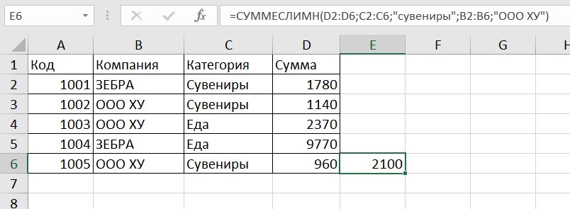
=СУММЕСЛИМН (D2: D6; C2: C6;”сувениры”; B2: B6;”ООО ХУ»)
D2: D6 — диапазон, где суммируются числа;
C2: C6 — диапазон ячеек для категории; сувениры — обязательное условие 1, то есть числа другой категории не учитываются;
B2: B6 — дополнительный диапазон;
ООО XY — условие 2, то есть числа другой компании не учитываются.
Дополнительных диапазонов и условий может быть до 127 штук.
СЧЕТ
=СЧЁТ (значение1; [значение2];…)Формула считает количество выбранных ячеек с числами в заданном диапазоне. Ячейки с датами тоже учитываются.
=СЧЁТ (значение1; [значение2];…)
Формула считает количество выбранных ячеек с числами в заданном диапазоне. Ячейки с датами тоже учитываются.
СЧЕТЕСЛИ и СЧЕТЕСЛИМН
=СЧЕТЕСЛИ (диапазон; критерий)
Функция определяет количество заполненных клеточек, которые подходят под конкретные условия в рамках указанного диапазона.
Например:
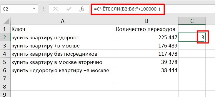
=СЧЁТЕСЛИМН (диапазон_условия1; условие1 [диапазон_условия2; условие2];…)
Эта формула позволяет использовать одновременно несколько критериев.
ЕСЛИОШИБКА
=ЕСЛИОШИБКА (значение; значение_если_ошибка)
Функция проверяет ошибочность значения или вычисления, а если ошибка отсутствует, возвращает его.
ДНИ
=ДНИ (конечная дата; начальная дата)
Функция показывает количество дней между двумя датами. В формуле указывают сначала конечную дату, а затем начальную.
КОРРЕЛ
=КОРРЕЛ (диапазон1; диапазон2)
Определяет статистическую взаимосвязь между разными данными: курсами валют, расходами и прибылью и т.д. Мах значение — +1, min — −1.
ВПР
=ВПР (искомое_значение; таблица; номер_столбца;[интервальный_просмотр])
Находит данные в таблице и диапазоне.
Например:
=ВПР (В1; С1: С26;2)
В1 — значение, которое ищем.
С1: Е26— диапазон, в котором ведется поиск.
2 — номер столбца для поиска.
ЛЕВСИМВ
=ЛЕВСИМВ (текст;[число_знаков])
Позволяет выделить нужное количество символов. Например, она поможет определить, поместится ли строка в лимитированное количество знаков или нет.
ПСТР
=ПСТР (текст; начальная_позиция; число_знаков)
Помогает достать определенное число знаков с текста. Например, можно убрать лишние слова в ячейках.
ПРОПИСН
=ПРОПИСН (текст)
Простая функция, которая делает все литеры в заданной строке прописными.
СТРОЧН
Функция, обратная предыдущей. Она делает все литеры строчными.
ПОИСКПОЗ
=ПОИСКПОЗ (искомое_значение; просматриваемый_массив; тип_сопоставления)
Дает возможность найти нужный элемент в заданном блоке ячеек и указывает его позицию.
ДЛСТР
=ДЛСТР (текст)
Данная функция определяет длину заданной строки. Пример использования — определение оптимальной длины описания статьи.
СЦЕПИТЬ
=СЦЕПИТЬ (текст1; текст2; текст3)
Позволяет сделать несколько строчек из одной и записать до 255 элементов (8192 символа).
ПРОПНАЧ
=ПРОПНАЧ (текст)
Позволяет поменять местами прописные и строчные символы.
ПЕЧСИМВ
=ПЕЧСИМВ (текст)
Можно убрать все невидимые знаки из текста.
Использование операторов
Операторы в Excel указывают, какие конкретно операции нужно выполнить над элементами формулы. В вычислениях всегда соблюдается математический порядок:
-
скобки;
-
экспоненты;
-
умножение и деление;
-
сложение и вычитание.
Арифметические
Операторы сравнения
Оператор объединения текста
Операторы ссылок

Использование ссылок
Начинающие пользователи обычно работают только с простыми ссылками, но мы расскажем обо всех форматах, даже продвинутых.
Простые ссылки A1
Они используются чаще всего. Буква обозначает столбец, цифра — строку.
Примеры:
-
диапазон ячеек в столбце С с 1 по 23 строку — «С1: С23»;
-
диапазон ячеек в строке 6 с B до Е– «B6: Е6»;
-
все ячейки в строке 11 — «11:11»;
-
все ячейки в столбцах от А до М — «А: М».
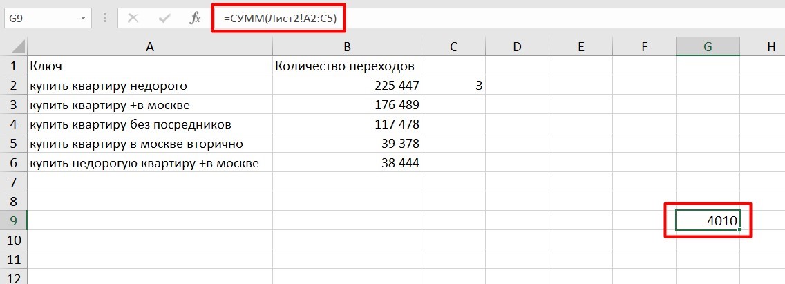
Ссылки на другой лист
Если необходимы данные с других листов, используется формула: =СУММ (Лист2! A5: C5)
Выглядит это так:
Абсолютные и относительные ссылки
Относительные ссылки
Рассмотрим, как они работают на примере: Напишем формулу для расчета суммы первой колонки. =СУММ (B4: B9)
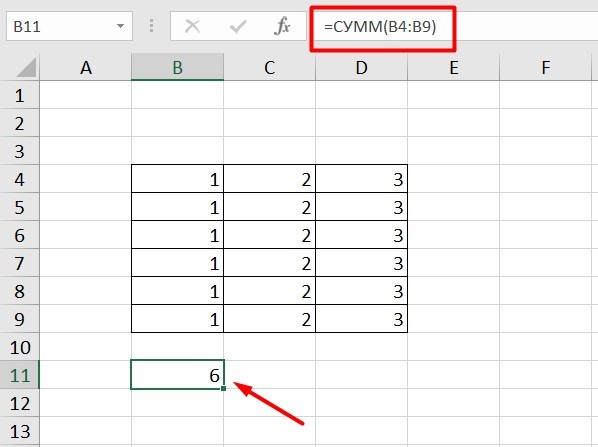
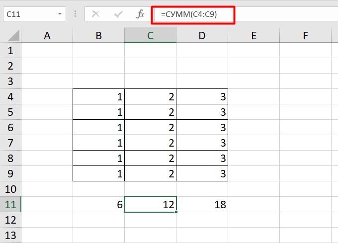
Нажимаем на Ctrl+C. Чтобы перенести формулу на соседнюю клетку, переходим туда и жмем на Ctrl+V. Или можно просто протянуть ячейку с формулой, как мы описывали выше.
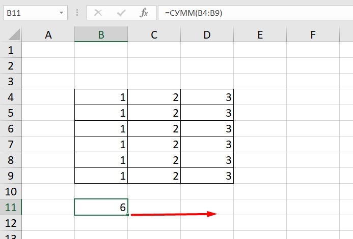
Индекс таблицы изменится автоматически и новые формулы будут выглядеть так:
Абсолютные ссылки
Чтобы при переносе формул ссылки сохранялись неизменными, требуются абсолютные адреса. Их пишут в формате «$B$2».
Например, есть поставить знак доллара в предыдущую формулу, мы получим: =СУММ ($B$4:$B$9)
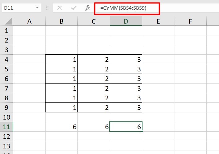
Как видите, никаких изменений не произошло.
Смешанные ссылки
Они используются, когда требуется зафиксировать только столбец или строку:
-
$А1– сохраняются столбцы;
-
А$1 — сохраняются строки.
Смешанные ссылки удобны, когда приходится работать с одной постоянной строкой данных и менять значения в столбцах. Или, когда нужно рассчитать результат в ячейках, не расположенных вдоль линии.
Трёхмерные ссылки
Это те, где указывается диапазон листов.
Формула выглядит примерно так: =СУММ (Лист1: Лист5! A6)
То есть будут суммироваться все ячейки А6 на всех листах с первого по пятый.
Ссылки формата R1C1
Номер здесь задается как по строкам, так и по столбцам.
Например:
-
R9C9 — абсолютная ссылка на клетку, которая расположена на девятой строке девятого столбца;
-
R[-2] — ссылка на строчку, расположенную выше на 2 строки;
-
R[-3]C — ссылка на клетку, которая расположена на 3 ячейки выше;
-
R[4]C[4] — ссылка на ячейку, которая распложена на 4 клетки правее и 4 строки ниже.
Использование имён
Функционал Excel позволяет давать собственные уникальные имена ячейкам, таблицам, константам, выражениям, даже диапазонам ячеек. Эти имена можно использовать для совершения любых арифметических действий, расчета налогов, процентов по кредиту, составления сметы и табелей, расчётов зарплаты, скидок, рабочего стажа и т.д.
Все, что нужно сделать — заранее дать имя ячейкам, с которыми планируете работать. В противном случае программа Эксель ничего не будет о них знать.
Как присвоить имя:
-
Выделите нужную ячейку/столбец.
-
Правой кнопкой мышки вызовите меню и перейдите в закладку «Присвоить имя».
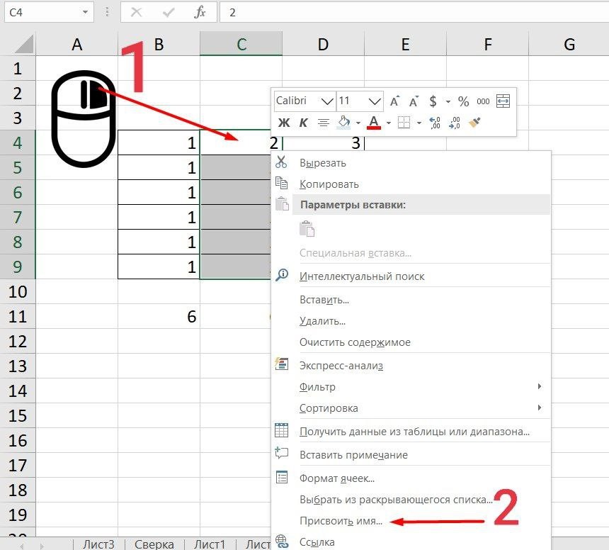
-
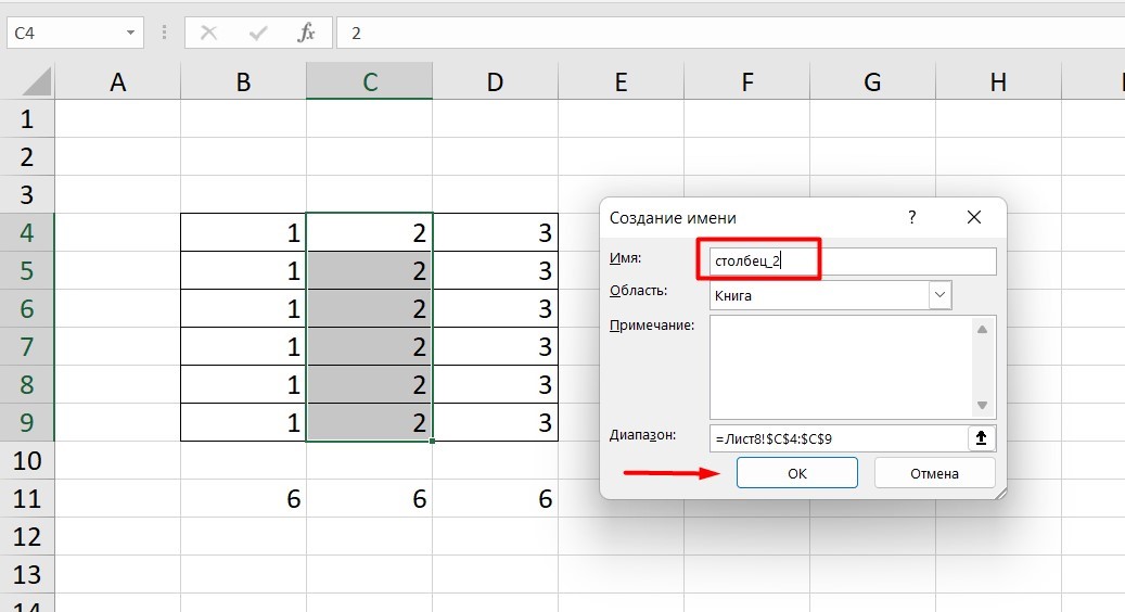
Напишите желаемое имя, которое должно быть уникальным и не повторяться в одной книге.
-
Сохраните, нажав Ок.
Использование функций
Чтобы вставить необходимую функцию в эксель-таблицах, можно использовать три способа: через панель инструментов, с помощью опции Вставки и вручную. Рассмотрим подробно каждый способ.
Ручной ввод
Этот способ подойдет тем, кто хорошо разбирается в теме и умеет создавать формулы прямо в строке. Для начинающих пользователей и новичков такой вариант покажется слишком сложным, поскольку надо все делать руками.
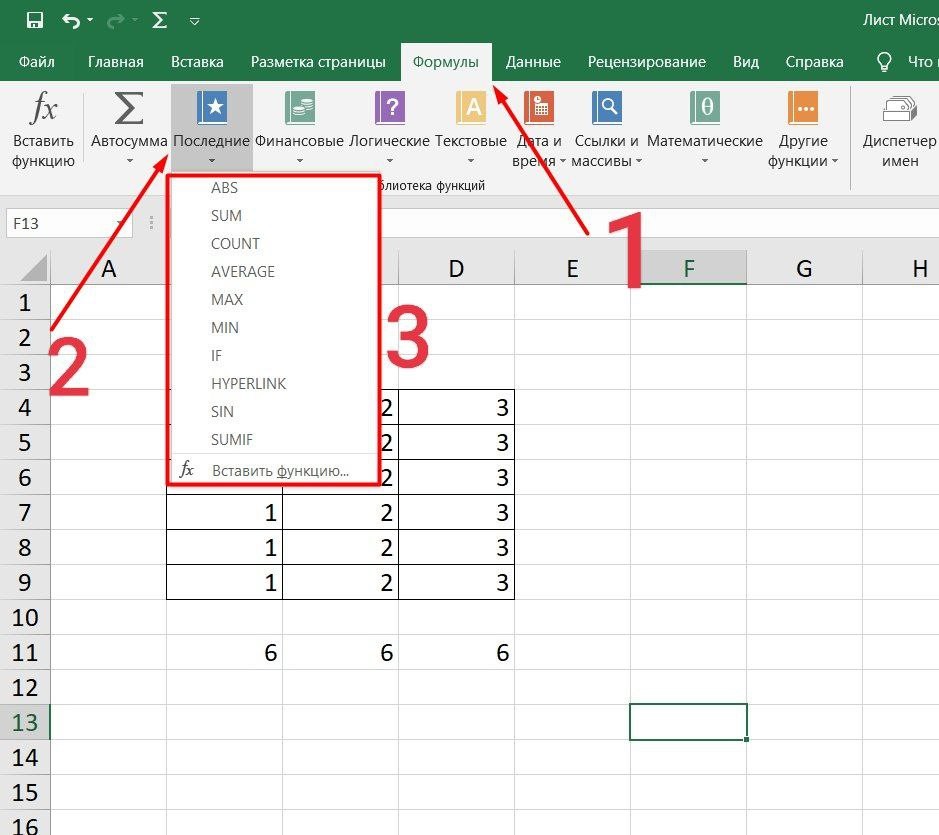
Панель инструментов
Это более упрощенный способ. Достаточно перейти в закладку «Формулы», выбрать подходящую библиотеку — Логические, Финансовые, Текстовые и др. (в закладке «Последние» будут наиболее востребованные формулы). Остается только выбрать из перечня нужную функцию и расставить аргументы.
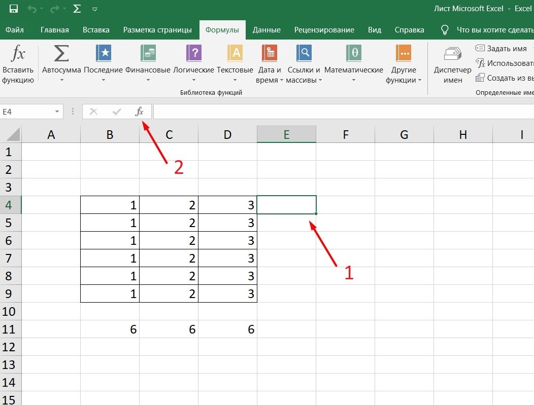
Мастер подстановки
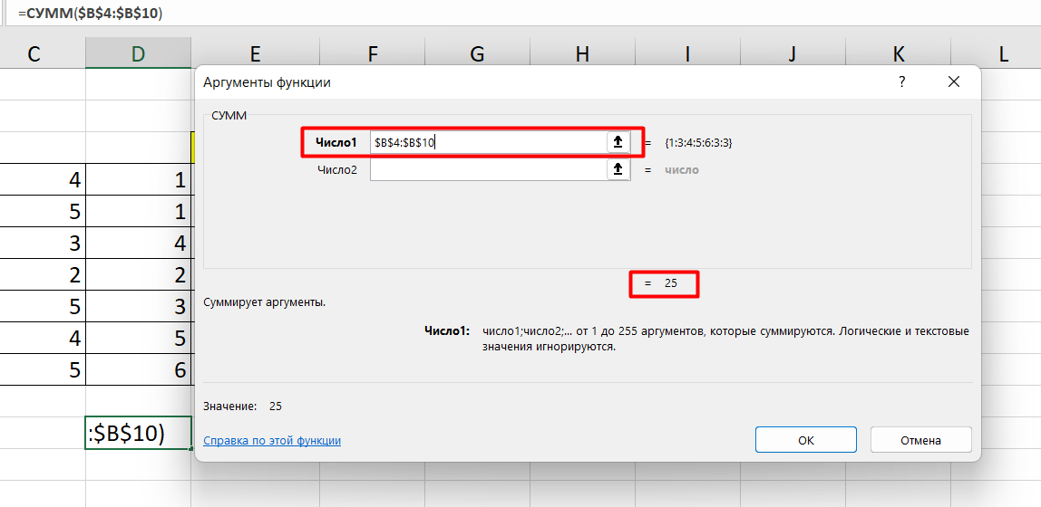
Кликните по любой ячейке в таблице. Нажмите на иконку «Fx», после чего откроется «Вставка функций».
Выберите из перечня нужную категорию формул, а затем кликните по функции, которую хотите применить и задайте необходимые для расчетов аргументы.
Вставка функции в формулу с помощью мастера
Рассмотрим эту опцию на примере:
-
Вызовите окошко «Вставка функции», как описывалось выше.
-
В перечне доступных функций выберите «Если».
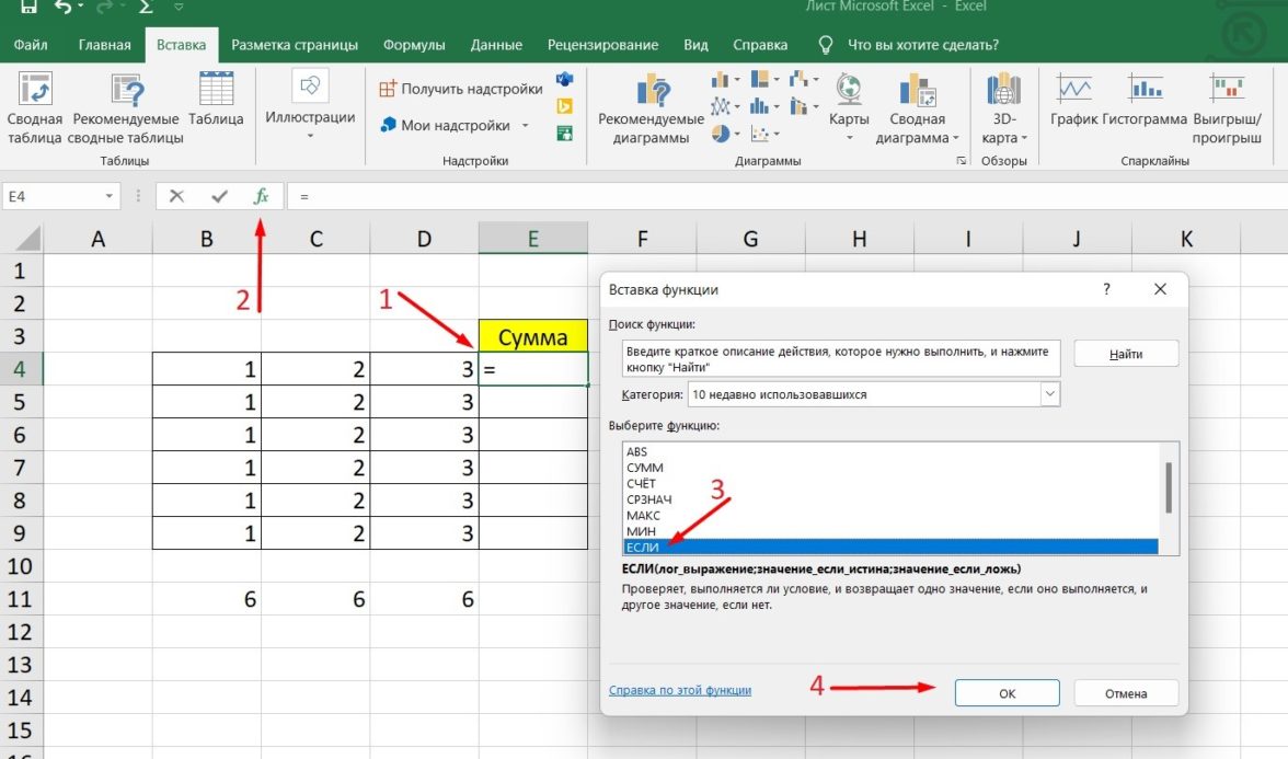
Теперь составим выражение, чтобы проверить, будет ли сумма трех ячеек больше 10. При этом Правда — «Больше 10», а Ложь — «Меньше 10».
=ЕСЛИ (СУММ (B3: D3)>10;”Больше 10″;»Меньше 10″)
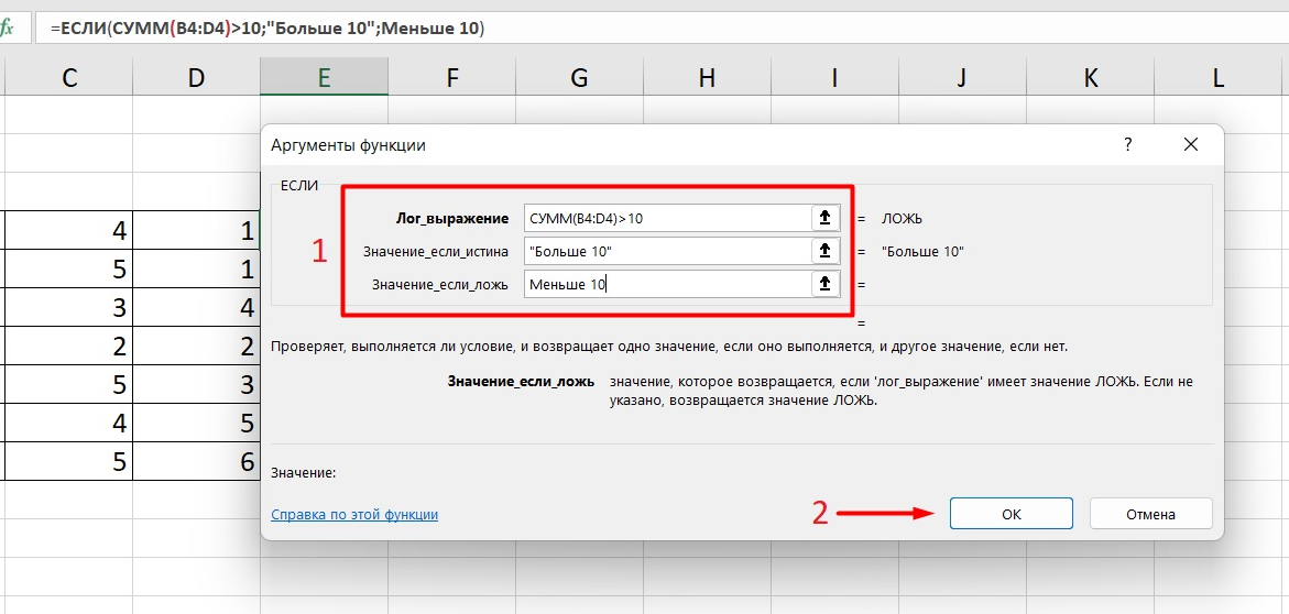
Программа посчитала, что сумма ячеек меньше 10 и выдала нам результат:
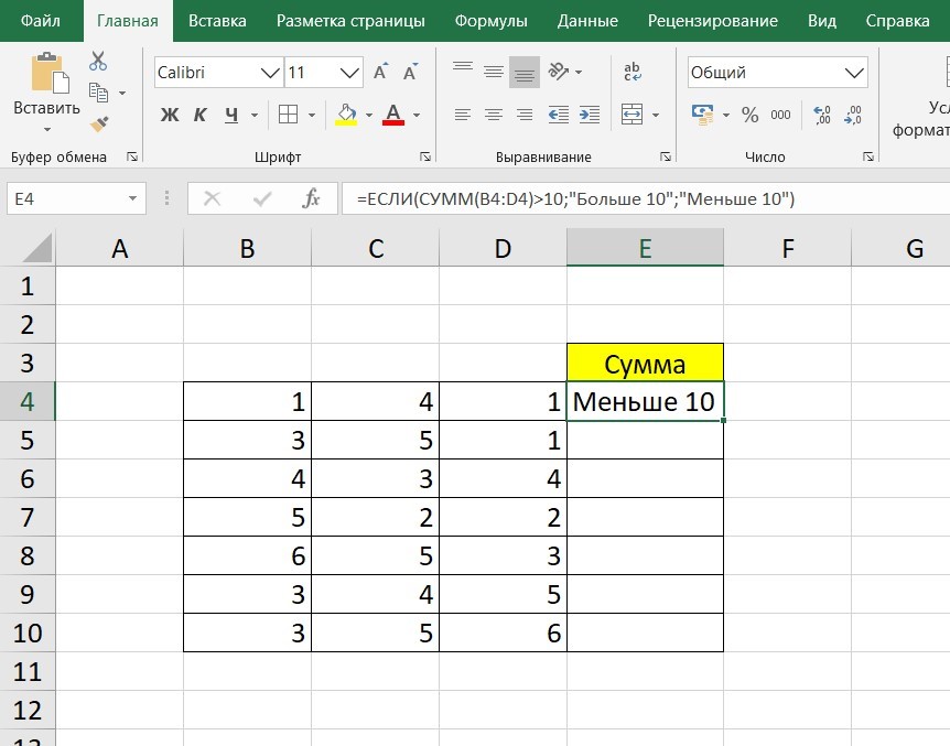
Чтобы получить значение в следующих ячейках столбца, нужно растянуть формулу (за правый нижний уголок). Получится следующее:
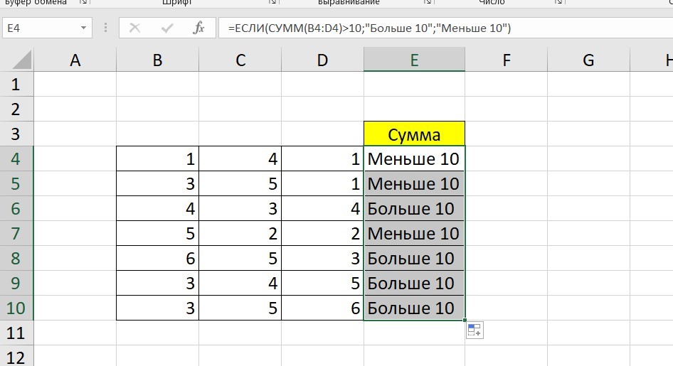
Мы использовали относительные ссылки, поэтому программа пересчитала выражение для всех строк корректно. Если бы нам нужно было зафиксировать адреса в аргументах, тогда мы бы применяли абсолютные ссылки, о которых писали выше.
Редактирование функций с помощью мастера
Чтобы отредактировать функцию, можно использовать два способа:
-
Строка формул. Для этого требуется перейти в специальное поле и вручную ввести необходимые изменения.
-
Специальный мастер. Нажмите на иконку «Fx» и в появившемся окошке измените нужные вам аргументы. И тут же, кстати, сможете узнать результат после редактирования.
Операции с формулами
С формулами можно совершать много операций — копировать, вставлять, перемещать. Как это делать правильно, расскажем ниже.
Копирование/вставка формулы
Чтобы скопировать формулу из одной ячейки в другую, не нужно изобретать велосипед — просто нажмите старую-добрую комбинацию (копировать), а затем кликните по новой ячейке и нажмите (вставить).
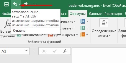
Отмена операций
Здесь вам в помощь стандартная кнопка «Отменить» на панели инструментов. Нажмите на стрелочку возле нее и выберите из контекстного меню те действия. которые хотите отменить.
Повторение действий
Если вы выполнили команду «Отменить», программа сразу активизирует функцию «Вернуть» (возле стрелочки отмены на панели). То есть нажав на нее, вы повторите только что отмененную вами операцию.
Стандартное перетаскивание
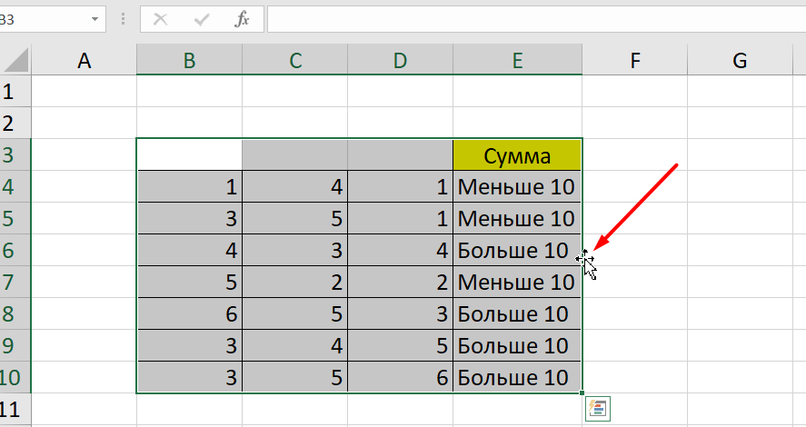
Выделенные ячейки переносятся с помощью указателя мышки в другое место листа. Делается это так:
-
Выделите фрагмент ячеек, которые нужно переместить.
-
Поместите указатель мыши над одну из границ фрагмента.
-
Когда указатель мыши станет крестиком с 4-мя стрелками, можете перетаскивать фрагмент в другое место.
Копирование путем перетаскивания
Если вам нужно скопировать выделенный массив ячеек в другое место рабочего листа с сохранением данных, делайте так:
-
Выделите диапазон ячеек, которые нужно скопировать.
-
Зажмите клавишу и поместите указатель мыши на границу выбранного диапазона.
-
Он станет похожим на крестик +. Это говорит о том, что будет выполняться копирование, а не перетаскивание.
-
Перетащите фрагмент в нужное место и отпустите мышку. Excel задаст вопрос — хотите вы заменить содержимое ячеек. Выберите «Отмена» или ОК.
Особенности вставки при перетаскивании
Если содержимое ячеек перемещается в другое место, оно полностью замещает собой существовавшие ранее записи. Если вы не хотите замещать прежние данные, удерживайте клавишу в процессе перетаскивания и копирования.
Автозаполнение формулами
Если необходимо скопировать одну формулу в массив соседних ячеек и выполнить массовые вычисления, используется функция автозаполнения.
Чтобы выполнить автозаполнение формулами, нужно вызвать специальный маркер заполнения. Для этого наведите курсор на нижний правый угол, чтобы появился черный крестик. Это и есть маркер заполнения. Его нужно зажать левой кнопкой мыши и протянуть вдоль всех ячеек, в которых вы хотите получить результат вычислений.
Как в формуле указать постоянную ячейку
Когда вам нужно протянуть формулу таким образом, чтобы ссылка на ячейку оставалась неизменной, делайте следующее:
-
Кликните на клетку, где находится формула.
-
Наведите курсор в нужную вам ячейку и нажмите F4.
-
В формуле аргумент с номером ячейки станет выглядеть так: $A$1 (абсолютная ссылка).
-
Когда вы протяните формулу, ссылка на ячейку $A$1 останется фиксированной и не будет меняться.
Как поставить «плюс», «равно» без формулы
Когда нужно указать отрицательное значение, поставить = или написать температуру воздуха, например, +22 °С, делайте так:
-
Кликаете правой кнопкой по ячейке и выбираете «Формат ячеек».
-
Отмечаете «Текстовый».
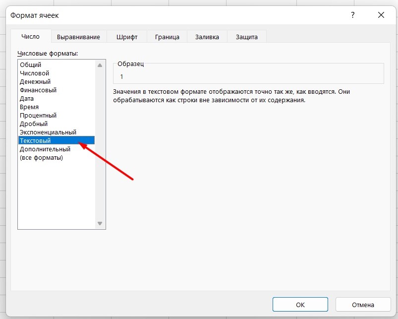
Теперь можно ставить = или +, а затем нужное число.
Самые распространенные ошибки при составлении формул в редакторе Excel
Новички, которые работают в редакторе Эксель совсем недавно, часто совершают элементарные ошибки. Поэтому рекомендуем ознакомиться с перечнем наиболее распространенных, чтобы больше не ошибаться.
-
Слишком много вложений в выражении. Лимит 64 штуки.
-
Пути к внешним книгам указаны не полностью. Проверяйте адреса более тщательно.
-
Неверно расставленные скобочки. В редакторе они обозначены разными цветами для удобства.
-
Указывая имена книг и листов, пользователи забывают брать их в кавычки.
-
Числа в неверном формате. Например, символ $ в Эксель — это не знак доллара, а формат абсолютных ссылок.
-
Неправильно введенные диапазоны ячеек. Не забывайте ставить «:».
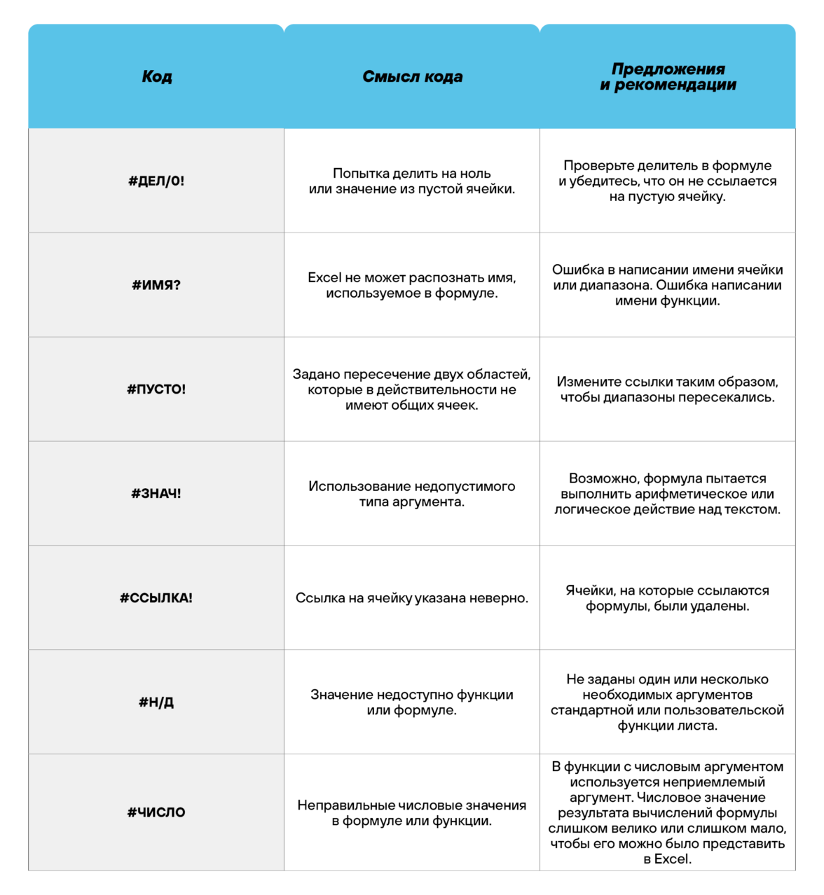
Коды ошибок при работе с формулами
Если вы сделаете ошибку в записи формулы, программа укажет на нее специальным кодом. Вот самые распространенные:
Отличие в версиях MS Excel
Всё, что написано в этом гайде, касается более современных версий программы 2007, 2010, 2013 и 2016 года. Устаревший Эксель заметно уступает в функционале и количестве доступных инструментов. Например, функция СЦЕП появилась только в 2016 году.
Во всем остальном старые и новые версии Excel не отличаются — операции и расчеты проводятся по одинаковым алгоритмам.
Заключение
Мы написали этот гайд, чтобы вам было легче освоить Excel. Доступным языком рассказали о формулах и о тех операциях, которые можно с ними проводить.
Надеемся, наша шпаргалка станет полезной для вас. Не забудьте сохранить ее в закладки и поделиться с коллегами.
Excel formulas allow you to identify relationships between values in your spreadsheet’s cells, perform mathematical calculations with those values, and return the resulting value in the cell of your choice. Sum, subtraction, percentage, division, average, and even dates/times are among the formulas that can be performed automatically. For example, =A1+A2+A3+A4+A5, which finds the sum of the range of values from cell A1 to cell A5.
Excel Functions: A formula is a mathematical expression that computes the value of a cell. Functions are predefined formulas that are already in Excel. Functions carry out specific calculations in a specific order based on the values specified as arguments or parameters. For example, =SUM (A1:A10). This function adds up all the values in cells A1 through A10.
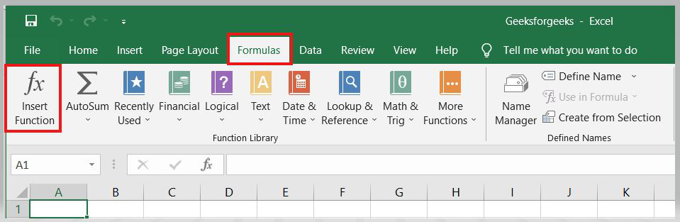
How to Insert Formulas in Excel?
This horizontal menu, shown below, in more recent versions of Excel allows you to find and insert Excel formulas into specific cells of your spreadsheet. On the Formulas tab, you can find all available Excel functions in the Function Library:
The more you use Excel formulas, the easier it will be to remember and perform them manually. Excel has over 400 functions, and the number is increasing from version to version. The formulas can be inserted into Excel using the following method:
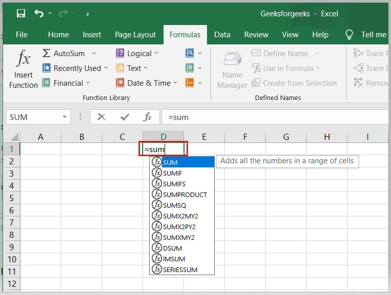
1. Simple insertion of the formula(Typing a formula in the cell):
Typing a formula into a cell or the formula bar is the simplest way to insert basic Excel formulas. Typically, the process begins with typing an equal sign followed by the name of an Excel function. Excel is quite intelligent in that it displays a pop-up function hint when you begin typing the name of the function.
2. Using the Insert Function option on the Formulas Tab:
If you want complete control over your function insertion, use the Excel Insert Function dialogue box. To do so, go to the Formulas tab and select the first menu, Insert Function. All the functions will be available in the dialogue box.
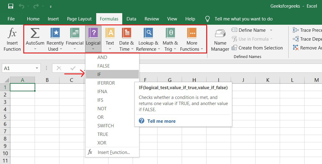
3. Choosing a Formula from One of the Formula Groups in the Formula Tab:
This option is for those who want to quickly dive into their favorite functions. Navigate to the Formulas tab and select your preferred group to access this menu. Click to reveal a sub-menu containing a list of functions. You can then choose your preference. If your preferred group isn’t on the tab, click the More Functions option — it’s most likely hidden there.
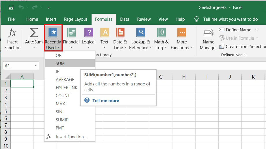
4. Use Recently Used Tabs for Quick Insertion:
If retyping your most recent formula becomes tedious, use the Recently Used menu. It’s on the Formulas tab, the third menu option after AutoSum.
Basic Excel Formulas and Functions:
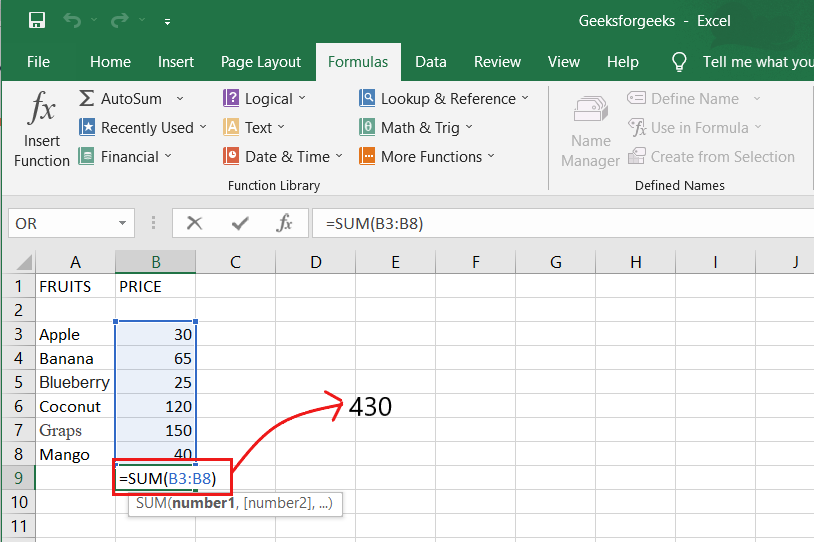
1. SUM:
The SUM formula in Excel is one of the most fundamental formulas you can use in a spreadsheet, allowing you to calculate the sum (or total) of two or more values. To use the SUM formula, enter the values you want to add together in the following format: =SUM(value 1, value 2,…..).
Example: In the below example to calculate the sum of price of all the fruits, in B9 cell type =SUM(B3:B8). this will calculate the sum of B3, B4, B5, B6, B7, B8 Press “Enter,” and the cell will produce the sum: 430.
2. SUBTRACTION:
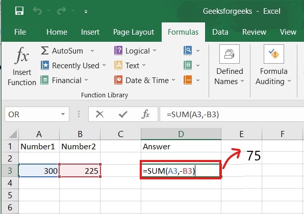
To use the subtraction formula in Excel, enter the cells you want to subtract in the format =SUM (A1, -B1). This will subtract a cell from the SUM formula by appending a negative sign before the cell being subtracted.
For example, if A3 was 300 and B3 was 225, =SUM(A1, -B1) would perform 300 + -225, returning a value of 75 in D3 cell.
3. MULTIPLICATION:
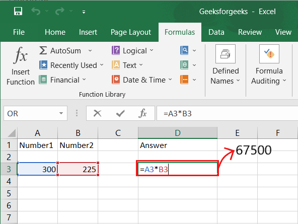
In Excel, enter the cells to be multiplied in the format =A3*B3 to perform the multiplication formula. An asterisk is used in this formula to multiply cell A3 by cell B3.
For example, if A3 was 300 and B3 was 225, =A1*B1 would return a value of 67500.
Highlight an empty cell in an Excel spreadsheet to multiply two or more values. Then, in the format =A1*B1…, enter the values or cells you want to multiply together. The asterisk effectively multiplies each value in the formula.
To return your desired product, press Enter. Take a look at the screenshot above to see how this looks.
4. DIVISION:
To use the division formula in Excel, enter the dividing cells in the format =A3/B3. This formula divides cell A3 by cell B3 with a forward slash, “/.”
For example, if A3 was 300 and B3 was 225, =A3/B3 would return a decimal value of 1.333333333.
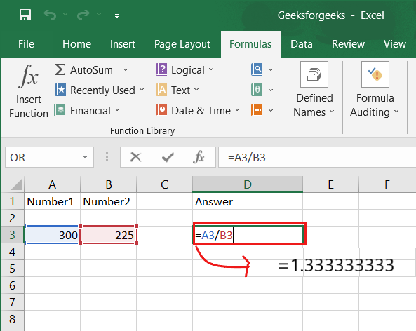
Division in Excel is one of the most basic functions available. To do so, highlight an empty cell, enter an equals sign, “=,” and then the two (or more) values you want to divide, separated by a forward slash, “/.” The output should look like this: =A3/B3, as shown in the screenshot above.
5. AVERAGE:
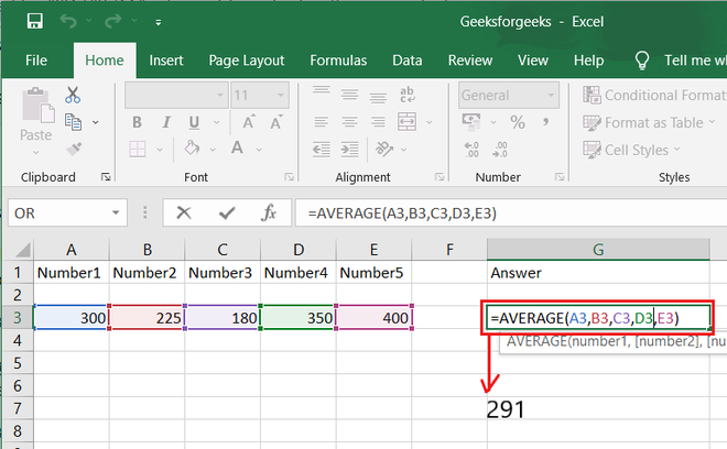
The AVERAGE function finds an average or arithmetic mean of numbers. to find the average of the numbers type = AVERAGE(A3.B3,C3….) and press ‘Enter’ it will produce average of the numbers in the cell.
For example, if A3 was 300, B3 was 225, C3 was 180, D3 was 350, E3 is 400 then =AVERAGE(A3,B3,C3,D3,E3) will produce 291.
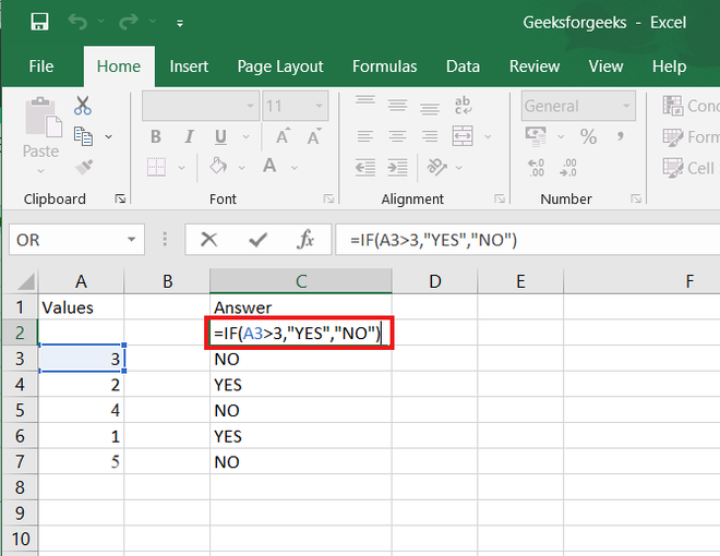
6. IF formula:
In Excel, the IF formula is denoted as =IF(logical test, value if true, value if false). This lets you enter a text value into a cell “if” something else in your spreadsheet is true or false.
For example, You may need to know which values in column A are greater than three. Using the =IF formula, you can quickly have Excel auto-populate a “yes” for each cell with a value greater than 3 and a “no” for each cell with a value less than 3.
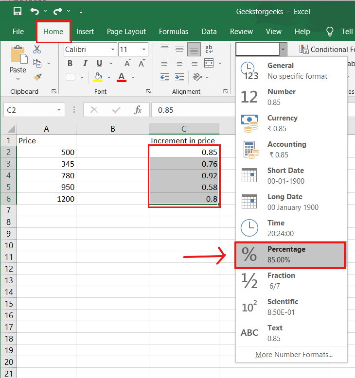
7. PERCENTAGE:
To use the percentage formula in Excel, enter the cells you want to calculate the percentage for in the format =A1/B1. To convert the decimal value to a percentage, select the cell, click the Home tab, and then select “Percentage” from the numbers dropdown.
There isn’t a specific Excel “formula” for percentages, but Excel makes it simple to convert the value of any cell into a percentage so you don’t have to calculate and reenter the numbers yourself.
The basic setting for converting a cell’s value to a percentage is found on the Home tab of Excel. Select this tab, highlight the cell(s) you want to convert to a percentage, and then select Conditional Formatting from the dropdown menu (this menu button might say “General” at first). Then, from the list of options that appears, choose “Percentage.” This will convert the value of each highlighted cell into a percentage. This feature can be found further down.
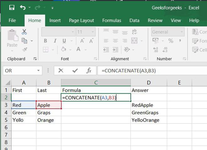
8. CONCATENATE:
CONCATENATE is a useful formula that combines values from multiple cells into the same cell.
For example , =CONCATENATE(A3,B3) will combine Red and Apple to produce RedApple.
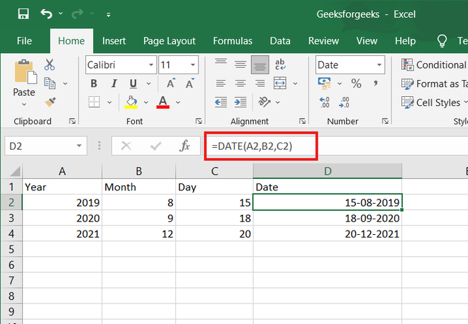
9. DATE:
DATE is the Excel DATE formula =DATE(year, month, day). This formula will return a date corresponding to the values entered in the parentheses, including values referred to from other cells.. For example, if A2 was 2019, B2 was 8, and C1 was 15, =DATE(A1,B1,C1) would return 15-08-2019.
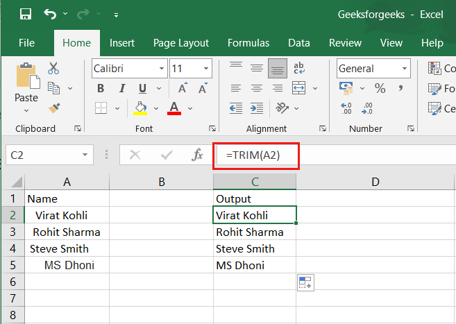
10. TRIM:
The TRIM formula in Excel is denoted =TRIM(text). This formula will remove any spaces that have been entered before and after the text in the cell. For example, if A2 includes the name ” Virat Kohli” with unwanted spaces before the first name, =TRIM(A2) would return “Virat Kohli” with no spaces in a new cell.
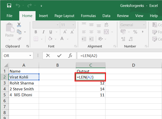
11. LEN:
LEN is the function to count the number of characters in a specific cell when you want to know the number of characters in that cell. =LEN(text) is the formula for this. Please keep in mind that the LEN function in Excel counts all characters, including spaces:
For example,=LEN(A2), returns the total length of the character in cell A2 including spaces.

How to Create a Simple Formula in Excel
To create a formula in excel must start with the equal sign “=”. If there is no equals sign, then whatever is typed in the cell will not be regarded as a formula.
Here’s how to create a simple formula, which is a formula for addition, subtraction, multiplication, and division. An addition formula using the plus sign “+”, subtraction formula using the negative sign “-“, a multiplication formula using an asterisk sign “*” and division formula using the slash “/”.
Addition Formula
There are two numbers in cell B1 and B2. How to create a formula in excel to add both of them?

There are several ways of writing a formula. The first way is using the keyboard and the arrow keys, the second way using the keyboard and mouse and a third way to use the keyboard by typing directly the formula and the address of cell involved.
For the above addition, the formula will be used the first way.
- Place the cursor in cell B4 and then type the equals sign “=”

- Press the up arrow button, point to cell B1, the cursor turns into dashed line.

- Type the plus sign “+” for the addition operation

- Press the up arrow button again, point to cell B2

- Press the ENTER key
The result is as shown below

Subtraction Formula
How to write a formula in excel for subtracting number1 by number2?. The reduction formula to use the second way, i.e. using the keyboard and mouse.
- Place the cursor in cell B5 and then type the equals sign “=”
- Click cell B1 using the mouse
- Type the negative sign “-” for the subtraction operation
- Click cell B2 using the mouse
- Press the ENTER key
For more details, you can see the animation below.
Multiplication Formula
How to make a formula in excel to multiply number1 by number2. For the multiplication formula using the third way of using the keyboard by writing directly the formula and the address of the cell involved.
- Place the cursor in cell B6 and then type the equals sign “=”
- Type B1
- Type an asterisk “*” for multiplication operations
- Type B2
- Press the ENTER key
For more details, you can see the animation below.
Division Formula
How to do formulas in excel to divide number1 with number2.
- Place the cursor in cell B7 and then type the equals sign “=”
- Point the cursor to cell B1
- Type a slash mark “/” for the division operation
- Point the cursor to cell B2
- Press the ENTER key
The result is as shown below

How to View Formulas in Excel
The easiest way to see the formula in a cell is to look at the formula bar. Point the cursor to a cell that contains a formula, then the formula bar will display the formula in the cell. The location of the formula bar is below the ribbon menu.

The picture above shows the formula contained in cell B4. To see formulas in other cells just move the cursor to the desired cell and see the formula in the formula bar.
Formula bar can only display formulas in the active cell, meaning only one formula can be shown. To be able to display all the formulas in a worksheet, please read the article below “How to Display Cell Formulas in Excel”
How to Edit Formula in Excel
There are two ways to edit a formula, using the F2 key or using a formula bar.
Editing with the F2 key
Place the cursor in the cell containing the formula, then press the F2 key. The contents of the formula will appear, and the cells involved in the formula will be marked with a colored box.
The picture below shows the existing addition formula in cell B4. There are two cells involved in the formula: cell B1 and B2. The address of the cell B1 light blue colored then the cell B1 will be surrounded with the same colored line, likewise with cell B2, the color of lines around it is same as cell B2 address color.

For example, the formula will be edited by adding the number 2. Type the plus sign “+”, number 2 and then press the ENTER key.
The results are as shown below. The formula in cell B4 has changed.

Editing with the formula bar
Place the cursor in the cell containing the formula, then click on the formula bar section. The formula in the cell will appear automatically. The display will be the same as when pressing the F2 key.
The picture below shows the existing subtraction formula in cell B5. For example, the formula will be edited by subtracting the number 2. Type a negative sign “-” number 2, then press the ENTER key.
How to Copy Formula in Excel
The cell that contains the formula can be copied like any other data. The difference, which is copied is the formula, not the value of the cell and the cell address forming the formula will be changed according to the location.
See image below. Cell B4 contains a formula that adds the value of cell B1 and B2. The formula will be copied and placed in the range C4: F4.

Place the cursor in cell B4. Do a copy (CTRL + C). Select C4: F4 range, then paste it (CTRL + V).
The result is as shown below.

The value of cell C4 to F4 is not equal to the value of cell B4, because excel copied the formula, not the cell value. Cell C4 contains a formula that adds C1 and C2 values, as well as cell D4 until F4; all contain a formula that adds cell values in row 1 and row 2 in the same column.
Another way to copy formula in excel
In addition to using the keyboard, there is another way to copy the formula, which is using the mouse. Eg formula in cell B5 will be copied. Click cell B5, point mouse to bottom right of cell B5 until the cursor change shape become thinner. Click and hold, then drag the cursor until cell F5. The result is as shown below.
Is there any other way to copy the formula with the mouse, of course 😊. For example, the formula in range B6: B7 will be copied. Select range B6: B7, then right click select copy. Select range C6: F7, right click, select Paste. The result as shown below.
How to Paste Special in Excel
If the cell that contains the formula is copied, the formulas are copied, not its value. The question is what if you want to copy the value, not the formulas. The solution is using Paste Special.
For example, there are data like the image above. Range A4:F7 mostly contains the formula, what if the range is copied and placed on the range A9:F11?.
Select range A4:F7. Do a copy (CTRL+C). Place the cursor in cell A9, and then do a paste (CTRL + V). The results are as shown below.

The results are different. If checked, cell B9 contains formula =B6+B7, as well as other cells in range B9:F12, all containing formulas.
For copying its value only. Select range A4:F7. Do a copy (CTRL+C). Place the cursor in cell A9, and then do a paste special (CTRL+ALT+V). A dialog box appears as shown below. Select “Values”, then click OK.

The results are shown below.

The results are equal to the range A4: F7. If rechecked, the content of cell B9 and other cells in the range B9:F12 is not a formula but a number.
How to Display Cell Formulas in Excel
To see the existing formula in a cell already discussed earlier. There is one drawback, only can see the formula in one cell only. If you want to see all the formulas that exist in the worksheet, the only way is to use the “Show Formulas” command.
The location is on Ribbon Menu, Formulas tab, auditing group formula. Click once, then all data generated from formula will show its formula. Click once again; it will return to its original state.
If you want to use the Show Formulas command faster, use the shortcut CTRL + ` (grave accent, in the left position of keyboard 1 and above the left tab)