

Use the Find and Replace features in Excel to search for something in your workbook, such as a particular number or text string. You can either locate the search item for reference, or you can replace it with something else. You can include wildcard characters such as question marks, tildes, and asterisks, or numbers in your search terms. You can search by rows and columns, search within comments or values, and search within worksheets or entire workbooks.

Find
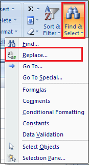
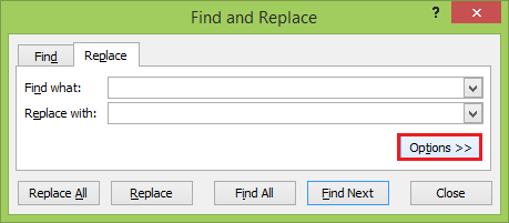
To find something, press Ctrl+F, or go to Home > Editing > Find & Select > Find.
Note: In the following example, we’ve clicked the Options >> button to show the entire Find dialog. By default, it will display with Options hidden.

-
In the Find what: box, type the text or numbers you want to find, or click the arrow in the Find what: box, and then select a recent search item from the list.
Tips: You can use wildcard characters — question mark (?), asterisk (*), tilde (~) — in your search criteria.
-
Use the question mark (?) to find any single character — for example, s?t finds «sat» and «set».
-
Use the asterisk (*) to find any number of characters — for example, s*d finds «sad» and «started».
-
Use the tilde (~) followed by ?, *, or ~ to find question marks, asterisks, or other tilde characters — for example, fy91~? finds «fy91?».
-
-
Click Find All or Find Next to run your search.
Tip: When you click Find All, every occurrence of the criteria that you are searching for will be listed, and clicking a specific occurrence in the list will select its cell. You can sort the results of a Find All search by clicking a column heading.
-
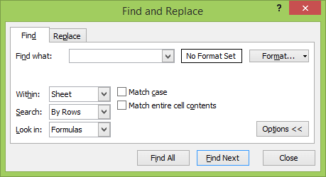
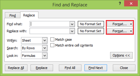
Click Options>> to further define your search if needed:
-
Within: To search for data in a worksheet or in an entire workbook, select Sheet or Workbook.
-
Search: You can choose to search either By Rows (default), or By Columns.
-
Look in: To search for data with specific details, in the box, click Formulas, Values, Notes, or Comments.
Note: Formulas, Values, Notes and Comments are only available on the Find tab; only Formulas are available on the Replace tab.
-
Match case — Check this if you want to search for case-sensitive data.
-
Match entire cell contents — Check this if you want to search for cells that contain just the characters that you typed in the Find what: box.
-
-
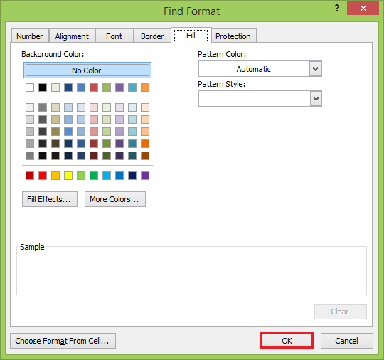
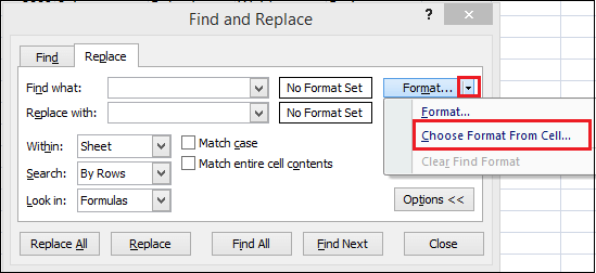
If you want to search for text or numbers with specific formatting, click Format, and then make your selections in the Find Format dialog box.
Tip: If you want to find cells that just match a specific format, you can delete any criteria in the Find what box, and then select a specific cell format as an example. Click the arrow next to Format, click Choose Format From Cell, and then click the cell that has the formatting that you want to search for.
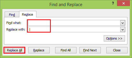
Replace
To replace text or numbers, press Ctrl+H, or go to Home > Editing > Find & Select > Replace.
Note: In the following example, we’ve clicked the Options >> button to show the entire Find dialog. By default, it will display with Options hidden.

-
In the Find what: box, type the text or numbers you want to find, or click the arrow in the Find what: box, and then select a recent search item from the list.
Tips: You can use wildcard characters — question mark (?), asterisk (*), tilde (~) — in your search criteria.
-
Use the question mark (?) to find any single character — for example, s?t finds «sat» and «set».
-
Use the asterisk (*) to find any number of characters — for example, s*d finds «sad» and «started».
-
Use the tilde (~) followed by ?, *, or ~ to find question marks, asterisks, or other tilde characters — for example, fy91~? finds «fy91?».
-
-
In the Replace with: box, enter the text or numbers you want to use to replace the search text.
-
Click Replace All or Replace.
Tip: When you click Replace All, every occurrence of the criteria that you are searching for will be replaced, while Replace will update one occurrence at a time.
-
Click Options>> to further define your search if needed:
-
Within: To search for data in a worksheet or in an entire workbook, select Sheet or Workbook.
-
Search: You can choose to search either By Rows (default), or By Columns.
-
Look in: To search for data with specific details, in the box, click Formulas, Values, Notes, or Comments.
Note: Formulas, Values, Notes and Comments are only available on the Find tab; only Formulas are available on the Replace tab.
-
Match case — Check this if you want to search for case-sensitive data.
-
Match entire cell contents — Check this if you want to search for cells that contain just the characters that you typed in the Find what: box.
-
-
If you want to search for text or numbers with specific formatting, click Format, and then make your selections in the Find Format dialog box.
Tip: If you want to find cells that just match a specific format, you can delete any criteria in the Find what box, and then select a specific cell format as an example. Click the arrow next to Format, click Choose Format From Cell, and then click the cell that has the formatting that you want to search for.
There are two distinct methods for finding or replacing text or numbers on the Mac. The first is to use the Find & Replace dialog. The second is to use the Search bar in the ribbon.
Find & Replace dialog
Search bar and options

-
Press Ctrl+F or go to Home > Find & Select > Find.
-
In Find what: type the text or numbers you want to find.
-
Select Find Next to run your search.
-
You can further define your search:
-
Within: To search for data in a worksheet or in an entire workbook, select Sheet or Workbook.
-
Search: You can choose to search either By Rows (default), or By Columns.
-
Look in: To search for data with specific details, in the box, click Formulas, Values, Notes, or Comments.
-
Match case — Check this if you want to search for case-sensitive data.
-
Match entire cell contents — Check this if you want to search for cells that contain just the characters that you typed in the Find what: box.
-
Tips: You can use wildcard characters — question mark (?), asterisk (*), tilde (~) — in your search criteria.
-
Use the question mark (?) to find any single character — for example, s?t finds «sat» and «set».
-
Use the asterisk (*) to find any number of characters — for example, s*d finds «sad» and «started».
-
Use the tilde (~) followed by ?, *, or ~ to find question marks, asterisks, or other tilde characters — for example, fy91~? finds «fy91?».

-
Press Ctrl+F or go to Home > Find & Select > Find.
-
In Find what: type the text or numbers you want to find.
-
Select Find All to run your search for all occurrences.

Note: The dialog box expands to show a list of all the cells that contain the search term, and the total number of cells in which it appears.
-
Select any item in the list to highlight the corresponding cell in your worksheet.
Note: You can edit the contents of the highlighted cell.

-
Press Ctrl+H or go to Home > Find & Select > Replace.
-
In Find what, type the text or numbers you want to find.
-
You can further define your search:
-
Within: To search for data in a worksheet or in an entire workbook, select Sheet or Workbook.
-
Search: You can choose to search either By Rows (default), or By Columns.
-
Match case — Check this if you want to search for case-sensitive data.
-
Match entire cell contents — Check this if you want to search for cells that contain just the characters that you typed in the Find what: box.
Tips: You can use wildcard characters — question mark (?), asterisk (*), tilde (~) — in your search criteria.
-
Use the question mark (?) to find any single character — for example, s?t finds «sat» and «set».
-
Use the asterisk (*) to find any number of characters — for example, s*d finds «sad» and «started».
-
Use the tilde (~) followed by ?, *, or ~ to find question marks, asterisks, or other tilde characters — for example, fy91~? finds «fy91?».
-
-
-
In the Replace with box, enter the text or numbers you want to use to replace the search text.
-
Select Replace or Replace All.
Tips:
-
When you select Replace All, every occurrence of the criteria that you are searching for is replaced.
-
When you select Replace, you can replace one instance at a time by selecting Next to highlight the next instance.
-
-
Select any cell to search the entire sheet or select a specific range of cells to search.
-
Press Command + F or select the magnifying glass to expand the Search bar and type the text or number you want to find in the search field.
Tips: You can use wildcard characters — question mark (?), asterisk (*), tilde (~) — in your search criteria.
-
Use the question mark (?) to find any single character — for example, s?t finds «sat» and «set».
-
Use the asterisk (*) to find any number of characters — for example, s*d finds «sad» and «started».
-
Use the tilde (~) followed by ?, *, or ~ to find question marks, asterisks, or other tilde characters — for example, fy91~? finds «fy91?».
-
-
Press return.
Notes:
-
To find the next instance of the item you are searching for, press return again or use the Find dialog box and select Find Next.
-
To specify additional search options, select the magnifying glass and select Search in Sheet or Search in Workbook. You can also select the Advanced option, which launches the Find dialog.
Tip: You can cancel a search in progress by pressing ESC.
-
Find
To find something, press Ctrl+F, or go to Home > Editing > Find & Select > Find.
Note: In the following example, we’ve clicked > Search Options to show the entire Find dialog. By default, it will display with Search Options hidden.

-
In the Find what: box, type the text or numbers you want to find.
Tips: You can use wildcard characters — question mark (?), asterisk (*), tilde (~) — in your search criteria.
-
Use the question mark (?) to find any single character — for example, s?t finds «sat» and «set».
-
Use the asterisk (*) to find any number of characters — for example, s*d finds «sad» and «started».
-
Use the tilde (~) followed by ?, *, or ~ to find question marks, asterisks, or other tilde characters — for example, fy91~? finds «fy91?».
-
-
Click Find Next or Find All to run your search.
Tip: When you click Find All, every occurrence of the criteria that you are searching for will be listed, and clicking a specific occurrence in the list will select its cell. You can sort the results of a Find All search by clicking a column heading.
-
Click > Search Options to further define your search if needed:
-
Within: To search for data within a certain selection, choose Selection. To search for data in a worksheet or in an entire workbook, select Sheet or Workbook.
-
Direction: You can choose to search either Down (default), or Up.
-
Match case — Check this if you want to search for case-sensitive data.
-
Match entire cell contents — Check this if you want to search for cells that contain just the characters that you typed in the Find what box.
-
Replace
To replace text or numbers, press Ctrl+H, or go to Home > Editing > Find & Select > Replace.
Note: In the following example, we’ve clicked > Search Options to show the entire Find dialog. By default, it will display with Search Options hidden.

-
In the Find what: box, type the text or numbers you want to find.
Tips: You can use wildcard characters — question mark (?), asterisk (*), tilde (~) — in your search criteria.
-
Use the question mark (?) to find any single character — for example, s?t finds «sat» and «set».
-
Use the asterisk (*) to find any number of characters — for example, s*d finds «sad» and «started».
-
Use the tilde (~) followed by ?, *, or ~ to find question marks, asterisks, or other tilde characters — for example, fy91~? finds «fy91?».
-
-
In the Replace with: box, enter the text or numbers you want to use to replace the search text.
-
Click Replace or Replace All.
Tip: When you click Replace All, every occurrence of the criteria that you are searching for will be replaced, while Replace will update one occurrence at a time.
-
Click > Search Options to further define your search if needed:
-
Within: To search for data within a certain selection, choose Selection. To search for data in a worksheet or in an entire workbook, select Sheet or Workbook.
-
Direction: You can choose to search either Down (default), or Up.
-
Match case — Check this if you want to search for case-sensitive data.
-
Match entire cell contents — Check this if you want to search for cells that contain just the characters that you typed in the Find what box.
-
Need more help?
You can always ask an expert in the Excel Tech Community or get support in the Answers community.
Recommended articles
Merge and unmerge cells
REPLACE, REPLACEB functions
Apply data validation to cells
How to Replace Text in Excel with the REPLACE function (2023)
Need to replace text in multiple cells?
Excel’s REPLACE and SUBSTITUTE functions make the process much easier.
Let’s take a look at how the two functions work, how they differ, and how you put them to use in a real spreadsheet🔍
If you want to follow along with what I show you, download my workbook here.
Replacing characters in text with the REPLACE function
The REPLACE function substitutes a text string with another text string.
Let’s say your boss tells you that the product IDs for a product line must be changed.
But only a part of the product ID should be changed – not all of it.

Here, the “29FA” part of all the product IDs needs to be changed to “39LU”.
To do that with the REPLACE function, we’ll walk through the syntax of the REPLACE function, which goes like this:
=REPLACE(old_text, start_num, num_chars, new_text)
Don’t worry, it’s not as daunting as it looks. It’s actually pretty straightforward👍
Step 1: Old text
The old text argument is a reference to the cell where you want to replace some text. Write:
=REPLACE(A2

And put a comma to wrap up the first argument, and let’s move on to the next.
Step 2: Start num
The start_num argument determines where the REPLACE function should start replacing characters from.
In our case, the “29FA” part starts on the 3rd character in the text.

So, write:
=REPLACE(A2, 3,
Now, we’ve established where the REPLACE function should start to replace text.
Still with me? Then let’s dive into the next argument of the REPLACE syntax🤿
Step 3: Num chars
Also called the “number of characters” argument, this determines how many characters should be replaced with the new text.
Typically, this should be the length of the text you want to replace the old text with.
So, it ties together with the next argument.
If you want to replace “29FA” with “39LU”, then you’re replacing the next 4 characters.
Write:
=REPLACE(A2, 3, 4

And wrap it up with a comma🎁
There are situations where this num_chars argument should be a different length than the new_text argument. I’ll tell you more about that later.
Step 4: New text
The new_text argument is the replacement text for the old text.
So, simply write the new characters that should replace the old 4 characters:
=REPLACE(A2, 3, 4, “39LU”

Remember the double quotes when the replacement text is letters or a combination of numbers and letters.
Wrap up the formula with an end parenthesis and press Enter.
Now, the “29FA” part of the old product ID is replaced with “39LU”.

PRO TIP: Length of num_chars vs new_text
If you need the replacement text to be shorter or longer than the text it’s replacing, you can have a different length in the 3rd and 4th argument of REPLACE. Let me give you a few formula examples of that:
If you wanted to replace the “29FA” with “39L” instead, you’d write:
=REPLACE(A2, 3, 4, “39L”)
But the length of the 4th argument would be shorter than the 4 characters defined in the 3rd argument.
On the other hand, if you wanted to replace “FA” with “LLUU”, you’d write this:
=REPLACE(A2, 5, 2, “LLUU”)

Replacing text strings with the SUBSTITUTE function
If the string you want to replace doesn’t always appear in the same place, you’re better off using the SUBSTITUTE function.
The syntax of SUBSTITUTE goes like this:
=SUBSTITUTE(text, old_text, new_text, [instance_num])
This is a little different from the last syntax of the REPLACE function, so be careful not to get them mixed up⚠️
Step 1: Text
The text argument is just a cell reference to the cell where you want to replace text.
Write:
=SUBSTITUTE(A2

And of course, put a comma to go to the next argument.
Step 2: Old text
The SUBSTITUTE function doesn’t replace characters from a fixed position in a cell.
Instead, it cleverly searches for a text string and begins replacing characters from there🔍
So, if you want to replace the “FA” part of the product ID with “LU”, write:
=SUBSTITUTE(A2, “FU”

Step 3: New text
The new_text argument is what the old text should be replaced with.
For this example, that’s “LU”.
=SUBSTITUTE(A2, “FA”, “LU”

The new text doesn’t have to be the same length as the old text.
Step 4: Instance num
The optional instance num argument decides how many times the text should be replaced.
This is relevant if there is more than one instance of the old text.
The instance_num argument is optional. If you leave it blank, every instance of the old text is replaced by the new text😊
In the following formula example, the first 2 product IDs each have 2 instances of the “FA”. So, the instance num argument determines whether only the first instance of “FA” is replaced with “LU” or both instances of “FA” is replaced with “LU”.
As you can see from the picture below, write 1 if you want only the first instance of “FA” to be replaced.
=SUBSTITUTE(A2, “FA”, “LU”, 1)
Or don’t use the instance num argument if every instance of “FA” should be replaced:
=SUBSTITUTE(A2, “FA”, “LU”)

And that’s how to replace text dynamically based on the location of the text you want to replace.
The difference between REPLACE and SUBSTITUTE
There are a few subtle differences between these two “replace functions”.
Both of them replace one or more characters in a text string with another text string.
The difference lies in how the first string is identified.
REPLACE selects the first string based on the position. So you might replace four characters, starting with the sixth character in the string.
SUBSTITUTE selects based on whether the string matches a predefined search. You might tell Excel to replace any instance of “FA” with “LU” for example.
Other than that, the two functions are identical👬🏻
Replace text using Find and Replace
Another way to replace text is with the ‘Find and Replace’ feature of Excel.
It’s a way to substitute characters in the original cell instead of having to add additional columns with formulas.
1. Select all the cells that contain the text to replace.
2. From the ‘Home’ tab, click ‘ Find and Select’.

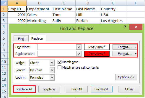
3. From the Find and Replace dialog box (in the replace tab) write the text you want to replace, in the ‘Find what:’ field.
4. Still within the ‘Find and Replace’ dialog box, write the new text to replace the old text with in the ‘Replace with:’ field.

5. When you click the ‘Replace all’ button, Excel replaces all instances of the old text with the new text, in the selected cells.
If you instead want to replace all instances of the text within the entire workbook, just select a single cell before opening the ‘Find and Replace’ dialog box.
(Instead of selecting multiple cells).
That’s it – Now what?
With the REPLACE and SUBSTITUTE functions, you can replace very specific strings with other strings. You can use letters, numbers, or other characters.
In short, you can replace text with extreme accuracy. And that saves you a great deal of time when you need to make a lot of edits.
Additionally, you can use the Find and Replace tool, which is the most underrated feature of Excel.
But no one got a job offer just based on their skills to replace characters in a text in Microsoft Excel.
Luckily, there are other areas of Excel that are magnets for job offers🧲
Click here to learn IF, SUMIF, VLOOKUP, and pivot tables (yup, that’s the magnets) for FREE in my 30-minute online Excel course.
Other resources
Replacing text is often used to clean up data so it’s ready for analysis, formulas, pivot tables, etc.
Other ways of cleaning up data are with other important Excel functions like LEFT, RIGHT, MID, and LEN.
Or with one of the two ways of deleting blank rows (one better than the other). Read all about it here.
Kasper Langmann2023-01-19T12:24:59+00:00
Page load link
When working with massive Excel data, it can be difficult and time-consuming to locate specific information or data.
In Excel, you can use the Find and Replace features to search for something in your workbooks, such as a particular number or text string. You can either locate the search item for reference or replace it with something else.
You can include wildcard characters such as question marks, tildes, asterisks, or numbers in your search terms. You can search by rows and columns, search within comments or values, and search within worksheets or entire workbooks.
How to use Find Feature
The following steps show you how to find specific characters, text, numbers, or dates in a range of cells, worksheets, or the entire workbook.
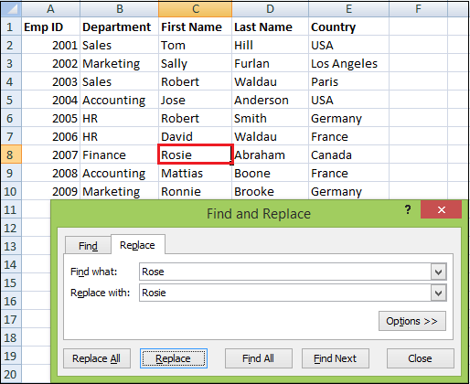
Consider an example in which we use the Find command to locate a specific department in this list.
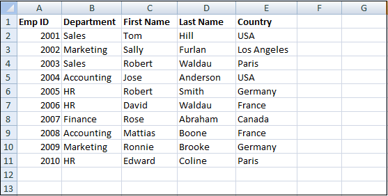
Step 1: Select the range of cells where you want to replace text or numbers. To replace characters across the entire worksheet, click any cell on the active sheet.
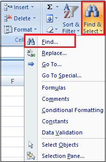
Step 2: Go to the Home tab and click on the Find & Select button in the ribbon’s Editing group.
Or you can open the Excel Find and Replace dialog by pressing the Ctrl + F shortcut key.
Step 3: The Find and Replace dialog box will appear.
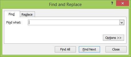
Step 4: In the Find what box, type the characters (text or number) you are looking for.
Step 5: Click either Find All or Find Next. If the content is found, then you will select the cell containing that content.
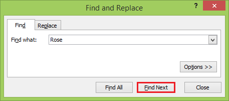
When you click Find Next, Excel selects the first occurrence of the search value on the sheet; the second click selects the second occurrence, and so on.
When you click Find All, Excel opens a list of all the occurrences, and you can click any item in the list to navigate to the corresponding cell.

Step 6: When you are finished, click Close to exit the Find and Replace dialog box.
Additional Options in Find Dialog Box
To fine-tune your search, click Options in the right-hand corner of the Excel Find & Replace dialog. It allows doing the following tasks, such as:
- To search for the specified value in the current worksheet or entire workbook, select Sheetor Workbook in the Within
- To search from the active cell from left to right (row-by-row), select By Rowsin the Search To search from top to bottom (column-by-column), select By Columns.
- To search among specific data types, select Formulas, Values, or Commentsin the Look in
- For a case-sensitive search, check the Match case check.
- To search for cells that contain only the characters you’ve entered in the Find whatfield, select the Match entire cell contents.
NOTE: If you want to find a given value in a range, column, or row, select that range, columns, or rows before opening Find and Replace in Excel. For example, limit your search to a specific column, select that column first, and then open the Find and Replace dialog.
How to Use Replace Feature
At times, you may discover that you’ve repeatedly made a mistake throughout your workbook, such as misspelling someone’s name or that you need to exchange a particular word or phrase for another. You can use Excel’s Find and Replace feature to make quick revisions.
To replace certain characters, texts, or numbers in an Excel sheet, use the Replace tab of the Excel Find & Replace dialog. You need to follow the following steps:
Step 1: Select the range of cells where you want to replace text or numbers. To replace characters across the entire worksheet, click any cell on the active sheet.
Step 2: Go to the Home tab, click on the Find & Select button and select the Replace feature.
Or Press the Ctrl + H shortcut key to open the Replace tab of the Excel Find and Replace dialog.

If you’ve just used the Excel Find feature, then switch to the Replace tab.
Step 3: In the Find what box, write the value to search for. And in the Replace with box, type the value to replace with.
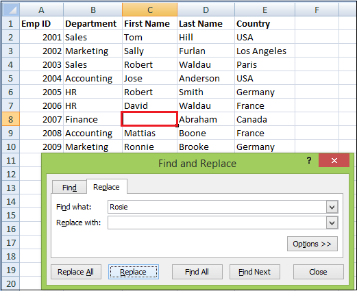
Step 4: Now, click either Replace to replace the found occurrences one by one or Replace All to swap all the entries in one fell swoop.
Step 5: When you are finished, click Close to exit the Find and Replace dialog box.
NOTE: If something has gone wrong and you got the result different from what you’d expected, click the Undo button or press Ctrl + Z to restore the original values.
Replace Data with Nothing
To replace all occurrences of a specific value with nothing, type the characters to search for in the Find what box, leave the Replace with box blank, and click the Replace All button.
How to Find or Replace a Line Break in Excel
To replace a line break with space or any other separator, enter the line break character in the Find what filed by pressing Ctrl + J. This shortcut is the ASCII control code for character 10 (line break or line feed).
After pressing Ctrl + J, the Find what box will look empty at first sight, but upon a closer look, you will notice a tiny flickering dot like in the screenshot below. Enter the replacement character in the Replace with box, e.g., a space character, and click Replace All.
To replace some character with a line break, do the opposite — enter the current character in the Find what box and the line break (Ctrl + J) in Replace with.
Excel Find and Replace with Wildcards
The use of wildcard characters in your search criteria can automate many finds and replace tasks in Excel:
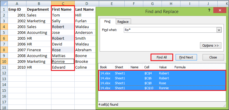
- Use the asterisk(*) to find any string of characters. For example, Ro* finds «Robert» and «Ronnie«.
- Use the question mark(?) to find any single character. For example, ?ose finds «Rose» and «Jose«.
For example, to get a list of first names that begin with «Ro«, use «Ro*» for the search criteria. Also, with the default options, Excel will search for the criteria anywhere in a cell.
In our worksheet, it would return all the cells that have «Ro» in any position. To prevent this from happening, click the Options button and check the Match entire cell contents box. This will force Excel to return only the values beginning with «ad«, as shown in the below screenshot.
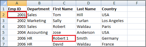
If you need to find actual asterisks or question marks in your Excel worksheet, type the tilde character (~) before them.
For example, to find cells that contain asterisks, you would type ~* in the Find what box. To find cells that have question marks, use ~? as your search criteria.
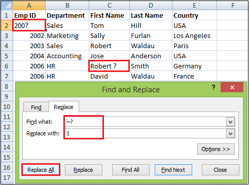
As you can see below, Excel successfully finds and replaces wildcards both in text and numeric values.
How to change cell formatting on the sheet
Excel Replace allows you to take a step further and change all cells’ formatting on the sheet or in the entire workbook. You have to follow the following steps:
Step 1: Click on the Find and Select button, and select the Replace feature.
Step 2: And click the Options button.
Step 3: Click on the Format button.
And specify the formatting you want to find or replace. Click the Ok button.
Or
Next to the Find what box, click on the arrow of the Format button.
Step 4: Select Choose Format From Cell and click on any cell with the format you want to change.
Step 5: Next to the Replace with box, either click the Format button and set the new format using the Excel Replace Format dialog box, or click the arrow of the Format button, select Choose Format From Cell, and click on any cell with the desired format.
Suppose you want to replace the formatting on the entire workbook, select workbook in the Within box. If you’re going to replace formatting on the active sheet only, leave the default selection.
Step 6: Finally, click the Replace All button and verify the result.
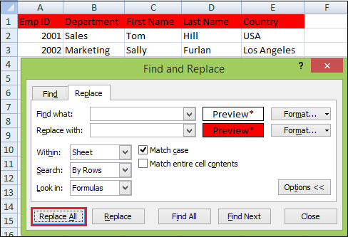
As a result, it replaced the entire first-row background with the selected red color font background.
NOTE: This method changes the formats applied manually. It will not work for conditionally formatted cells.
Advanced Find and Replace Features
In Excel, Advance Find and Replace are used to find and replace in all open workbooks, add-in by Ablebits. The following Advanced Find and Replace features make a search in Excel even more powerful, such as:
- Find and Replace in all open workbooksor selected workbooks & worksheets.
- Simultaneous search in values, formulas, hyperlinks, and comments.
- We are exporting search results to a new workbook.
Follows the following steps to run the Advanced Find and Replace add-in in Excel:
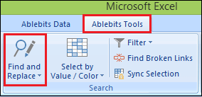
Step 1: Click on the Excel ribbon icon, which resides on the Ablebits Tools tab.
Step 2: Go to the Search group and click the Find and Replace button. You can also press Ctrl + Alt + F or even configure it to open by the familiar Ctrl + F shortcut.
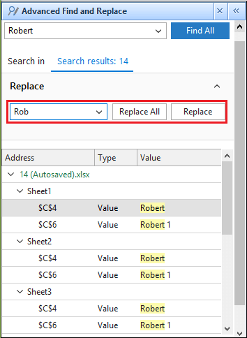
The Advanced Find and Replace pane will open, and you do the following:
- Type the characters (text or number) to search for in the Find what
- Select which workbooks and worksheets you want to search. By default, all sheets in all open workbooks are selected.
- Choose what data types to look in: values, formulas, comments, or hyperlinks. By default, all data types are selected.
- Select the Match caseoption to look for case-sensitive data.
- Select the Entire cell check box to search for an exact and complete match, i.e., find cells that contain only the characters you’ve typed in the Find what
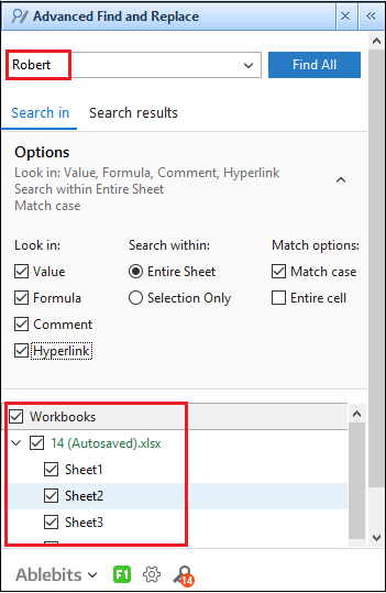
Step 3: Click the Find All button, and you will see a list of found entries on the search results tab.
Step 4: And now, you can replace all or selected occurrences with some other value or export the found cells, rows, or columns to a new workbook.
Step 5: Click on the Replace All button.
Step 6: Click on the Export all button or select according to your need.
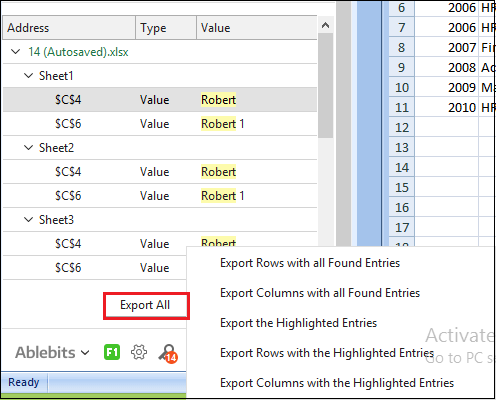
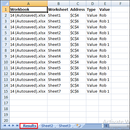
As a result, it creates a result workbook, as shown below.
Replace Function in Excel
The REPLACE function in Excel allows you to swap one or several characters in a text string with another character or a set of characters. Below is the basic syntax of Replace function.
The Excel REPLACE function has four arguments, all of which are required.
- Old_text: The original text or a reference to a cell with the original text in which you want to replace some characters.
- Start_num: The position of the first character within old_text that you want to replace.
- Num_chars: The number of characters you want to replace.
- New_text: The replacement text.
NOTE: If the start_num or num_chars argument is negative or non-numeric, an Excel Replace formula returns the error (#VALUE!).
Содержание
- Examples of working with text function REPLACE in Excel
- How does the REPLACE function in Excel work?
- REPLACE function in Excel and examples of its use
- How to REPLACE a piece of text in Excel cell?
- REPLACE, REPLACEB functions
- Description
- Syntax
- Example
- Find or replace text and numbers on a worksheet
- Replace
- SUBSTITUTE Function
- Related functions
- Summary
- Purpose
- Return value
- Arguments
- Syntax
- Usage notes
- Examples
- Related functions
- How to find and replace multiple values at once in Excel (bulk replace)
- Find and replace multiple values with nested SUBSTITUTE
- Search and replace multiple entries with XLOOKUP
- Multiple replace using recursive LAMBDA function
- Example 1. Search and replace multiple words / strings at once
- Example 2. Replace multiple characters in Excel
- Mass find and replace with UDF
- Bulk replace in Excel with VBA macro
- How to use the macro
- Multiple find and replace in Excel with Substring tool
Examples of working with text function REPLACE in Excel
REPLACE function is included in the text functions of MS Excel and is intended to replace a specific area of the text string containing the source text on the specified text line (new text).
How does the REPLACE function in Excel work?
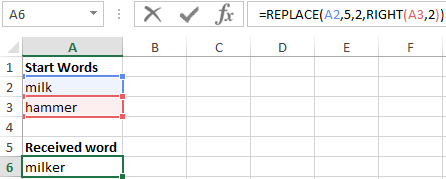
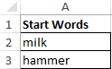
Example 1. In order to study in detail the operation of this function, we consider one of the simplest examples. Suppose we have several words in different columns, we need to get new words using the original ones. For this example, in addition to our main function REPLACE, we also use the RIGHT function — this function serves to return a certain number of characters from the end of a line of text. That is, for example, we have two words: milk and a skating rink, as a result we must get the word hammer.
REPLACE function in Excel and examples of its use
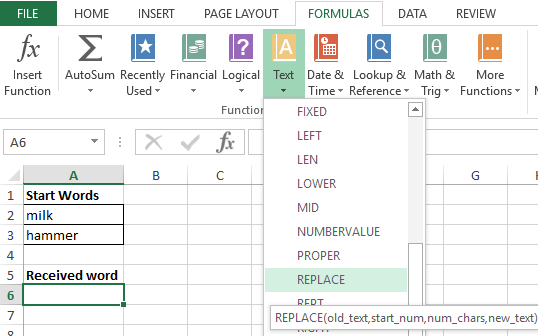
- Create a table with words on the sheet of the Excel spreadsheet workbook, as shown in the figure:
- Next, on the sheet of the workbook, we will prepare an area for placing our result — the resulting word “hammer”, as shown below. Place the cursor in cell A6 and call the function REPLACE:
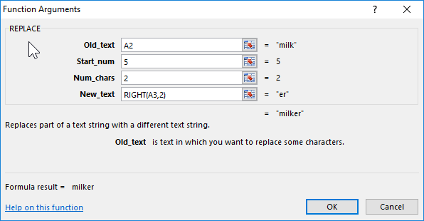
- Fill the function with the arguments shown in the figure:
Let us explain the choice of these parameters as follows: cell A2 was chosen as the beginning of the text, the number 5 was set as beginning_, since it is from the fifth position of the word “Milk” we don’t take characters for our final word, the number_ of signs was set equal to 2, since this number It is not taken into account in the new word, as the new text, the set option RIGHT with the parameters of the cell A3 and taking the last two characters «ok».
Next, click on the «OK» button and get the result:
How to REPLACE a piece of text in Excel cell?
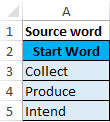
Example 2. Consider another small example. Suppose we have columns of words in the cells of the Excel spreadsheet. It is necessary to replace their letters in certain places so as to convert them.
- Let’s create a tablet with words on the sheet of an Excel workbook, as shown in the figure:
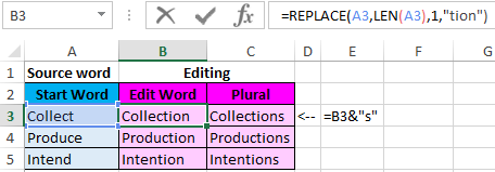
- Further, on the same sheet of the working book we will prepare an area for placing our result — modified words. Fill the cells with two types of formulas as shown in the picture:
Note! In the second formula, we use the operator “&” to add the character «s» to the male surname to convert it to the female. To solve this problem, one could use the function =CONCATENATE(B3,»s») instead of the formula =B3&»s» — the result is identical. But today it is strongly recommended to abandon this formula as it has its limitations and is more demanding on resources in comparison with a simple and convenient ampersand operator.
Источник
REPLACE, REPLACEB functions
This article describes the formula syntax and usage of the REPLACE and REPLACEB function in Microsoft Excel.
Description
REPLACE replaces part of a text string, based on the number of characters you specify, with a different text string.
REPLACEB replaces part of a text string, based on the number of bytes you specify, with a different text string.
These functions may not be available in all languages.
REPLACE is intended for use with languages that use the single-byte character set (SBCS), whereas REPLACEB is intended for use with languages that use the double-byte character set (DBCS). The default language setting on your computer affects the return value in the following way:
REPLACE always counts each character, whether single-byte or double-byte, as 1, no matter what the default language setting is.
REPLACEB counts each double-byte character as 2 when you have enabled the editing of a language that supports DBCS and then set it as the default language. Otherwise, REPLACEB counts each character as 1.
The languages that support DBCS include Japanese, Chinese (Simplified), Chinese (Traditional), and Korean.
Syntax
REPLACE(old_text, start_num, num_chars, new_text)
REPLACEB(old_text, start_num, num_bytes, new_text)
The REPLACE and REPLACEB function syntax has the following arguments:
Old_text Required. Text in which you want to replace some characters.
Start_num Required. The position of the character in old_text that you want to replace with new_text.
Num_chars Required. The number of characters in old_text that you want REPLACE to replace with new_text.
Num_bytes Required. The number of bytes in old_text that you want REPLACEB to replace with new_text.
New_text Required. The text that will replace characters in old_text.
Example
Copy the example data in the following table, and paste it in cell A1 of a new Excel worksheet. For formulas to show results, select them, press F2, and then press Enter. If you need to, you can adjust the column widths to see all the data.
Источник
Find or replace text and numbers on a worksheet
Use the Find and Replace features in Excel to search for something in your workbook, such as a particular number or text string. You can either locate the search item for reference, or you can replace it with something else. You can include wildcard characters such as question marks, tildes, and asterisks, or numbers in your search terms. You can search by rows and columns, search within comments or values, and search within worksheets or entire workbooks.
Tip: You can also use formulas to replace text. Check out the SUBSTITUTE function or REPLACE, REPLACEB functions to learn more.
To find something, press Ctrl+F, or go to Home > Editing > Find & Select > Find.
Note: In the following example, we’ve clicked the Options >> button to show the entire Find dialog. By default, it will display with Options hidden.
In the Find what: box, type the text or numbers you want to find, or click the arrow in the Find what: box, and then select a recent search item from the list.
Tips: You can use wildcard characters — question mark ( ?), asterisk ( *), tilde (
) — in your search criteria.
Use the question mark (?) to find any single character — for example, s?t finds «sat» and «set».
Use the asterisk (*) to find any number of characters — for example, s*d finds «sad» and «started».
) followed by ?, *, or
to find question marks, asterisks, or other tilde characters — for example, fy91
Click Find All or Find Next to run your search.
Tip: When you click Find All, every occurrence of the criteria that you are searching for will be listed, and clicking a specific occurrence in the list will select its cell. You can sort the results of a Find All search by clicking a column heading.
Click Options>> to further define your search if needed:
Within: To search for data in a worksheet or in an entire workbook, select Sheet or Workbook.
Search: You can choose to search either By Rows (default), or By Columns.
Look in: To search for data with specific details, in the box, click Formulas, Values, Notes, or Comments.
Note: Formulas, Values, Notes and Comments are only available on the Find tab; only Formulas are available on the Replace tab.
Match case — Check this if you want to search for case-sensitive data.
Match entire cell contents — Check this if you want to search for cells that contain just the characters that you typed in the Find what: box.
If you want to search for text or numbers with specific formatting, click Format, and then make your selections in the Find Format dialog box.
Tip: If you want to find cells that just match a specific format, you can delete any criteria in the Find what box, and then select a specific cell format as an example. Click the arrow next to Format, click Choose Format From Cell, and then click the cell that has the formatting that you want to search for.
Replace
To replace text or numbers, press Ctrl+H, or go to Home > Editing > Find & Select > Replace.
Note: In the following example, we’ve clicked the Options >> button to show the entire Find dialog. By default, it will display with Options hidden.
In the Find what: box, type the text or numbers you want to find, or click the arrow in the Find what: box, and then select a recent search item from the list.
Tips: You can use wildcard characters — question mark ( ?), asterisk ( *), tilde (
) — in your search criteria.
Use the question mark (?) to find any single character — for example, s?t finds «sat» and «set».
Use the asterisk (*) to find any number of characters — for example, s*d finds «sad» and «started».
) followed by ?, *, or
to find question marks, asterisks, or other tilde characters — for example, fy91
In the Replace with: box, enter the text or numbers you want to use to replace the search text.
Click Replace All or Replace.
Tip: When you click Replace All, every occurrence of the criteria that you are searching for will be replaced, while Replace will update one occurrence at a time.
Click Options>> to further define your search if needed:
Within: To search for data in a worksheet or in an entire workbook, select Sheet or Workbook.
Search: You can choose to search either By Rows (default), or By Columns.
Look in: To search for data with specific details, in the box, click Formulas, Values, Notes, or Comments.
Note: Formulas, Values, Notes and Comments are only available on the Find tab; only Formulas are available on the Replace tab.
Match case — Check this if you want to search for case-sensitive data.
Match entire cell contents — Check this if you want to search for cells that contain just the characters that you typed in the Find what: box.
If you want to search for text or numbers with specific formatting, click Format, and then make your selections in the Find Format dialog box.
Tip: If you want to find cells that just match a specific format, you can delete any criteria in the Find what box, and then select a specific cell format as an example. Click the arrow next to Format, click Choose Format From Cell, and then click the cell that has the formatting that you want to search for.
There are two distinct methods for finding or replacing text or numbers on the Mac. The first is to use the Find & Replace dialog. The second is to use the Search bar in the ribbon.
Источник
SUBSTITUTE Function
Summary
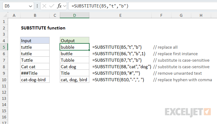
The Excel SUBSTITUTE function replaces text in a given string by matching. For example =SUBSTITUTE(«952-455-7865″,»-«,»») returns «9524557865»; the dash is stripped. SUBSTITUTE is case-sensitive and does not support wildcards.
Purpose
Return value
Arguments
- text — The text to change.
- old_text — The text to replace.
- new_text — The text to replace with.
- instance — [optional] The instance to replace. If not supplied, all instances are replaced.
Syntax
Usage notes
The Excel SUBSTITUTE function can replace text by matching. Use the SUBSTITUTE function when you want to replace text based on matching, not position. Optionally, you can specify the instance of found text to replace (i.e. first instance, second instance, etc.).
SUBSTITUTE is case-sensitive. To replace one or more characters with nothing, enter an empty string («»).
Examples
Below are the formulas used in the example shown above:
The SUBSTITUTE function cannot replace more than one string at a time. However, SUBSTITUTE can be nested inside of itself to accomplish the same thing. For example, with the text «a (dog)» in cell A1, the formula below will strip parentheses () from text:
This same approach can be used in a more complex formula to normalize telephone numbers.
Use the REPLACE function to replace text at a known location in a text string. Use the SUBSTITUTE function to replace text by searching when the location is not known. Use FIND or SEARCH to determine the location of specific text.
Источник
How to find and replace multiple values at once in Excel (bulk replace)
 by Svetlana Cheusheva, updated on March 13, 2023
In this tutorial, we will look at several ways to find and replace multiple words, strings, or individual characters, so you can choose the one that best suits your needs.
How do people usually search in Excel? Mostly, by using the Find & Replace feature, which works fine for single values. But what if you have tens or even hundreds of items to replace? Surely, no one would want to make all those replacements manually one-by-one, and then do it all over again when the data changes. Luckily, there are a few more effective methods to do mass replace in Excel, and we are going to investigate each of them in detail.
Find and replace multiple values with nested SUBSTITUTE
The easiest way to find and replace multiple entries in Excel is by using the SUBSTITUTE function.
The formula’s logic is very simple: you write a few individual functions to replace an old value with a new one. And then, you nest those functions one into another, so that each subsequent SUBSTITUTE uses the output of the previous SUBSTITUTE to look for the next value.
In the list of locations in A2:A10, suppose you want to replace the abbreviated country names (such as FR, UK and USA) with full names.
To have it done, enter the old values in D2:D4 and the new values in E2:E4 like shown in the screenshot below. And then, put the below formula in B2 and press Enter:
=SUBSTITUTE(SUBSTITUTE(SUBSTITUTE(A2:A10, D2, E2), D3, E3), D4, E4)
…and you will have all the replacements done at once: 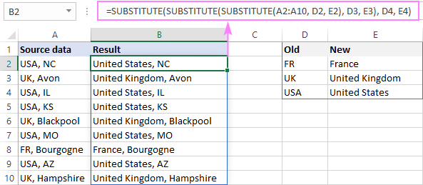
Please note, the above approach only works in Excel 365 that supports dynamic arrays.
In pre-dynamic versions of Excel 2019, Excel 2016 and earlier, the formula needs to be written for the topmost cell (B2), and then copied to the below cells:
=SUBSTITUTE(SUBSTITUTE(SUBSTITUTE(A2, $D$2, $E$2), $D$3, $E$3), $D$4, $E$4)
Please pay attention that, in this case, we lock the replacement values with absolute cell references, so they won’t shift when copying the formula down. 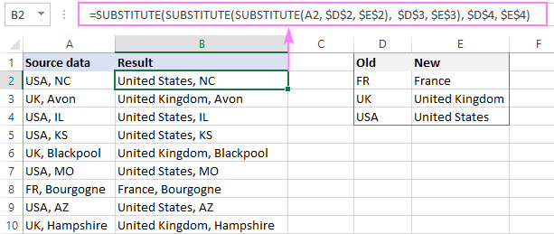
Note. The SUBSTITUTE function is case-sensitive, meaning you should type the old values (old_text) in the same letter case as they appear in the original data.
As easy as it could possibly be, this method has a significant drawback — when you have dozens of items to replace, nested functions become quite difficult to manage.
Advantages: easy-to-implement; supported in all Excel versions
Drawbacks: best to be used for a limited number of find/replace values
Search and replace multiple entries with XLOOKUP
In situation when you are looking to replace the entire cell content, not its part, the XLOOKUP function comes in handy.
Let’s say you have a list of countries in column A and aim to replace all the abbreviations with the corresponding full names. Like in the previous example, you start with inputting the «Find» and «Replace» items in separate columns (D and E respectively), and then enter this formula in B2:
=XLOOKUP(A2, $D$2:$D$4, $E$2:$E$4, A2)
Translated from the Excel language into the human language, here’s what the formula does:
Search for the A2 value (lookup_value) in D2:D4 (lookup_array) and return a match from E2:E4 (return_array). If not found, pull the original value from A2.
Double-click the fill handle to get the formula copied to the below cells, and the result won’t keep you waiting: 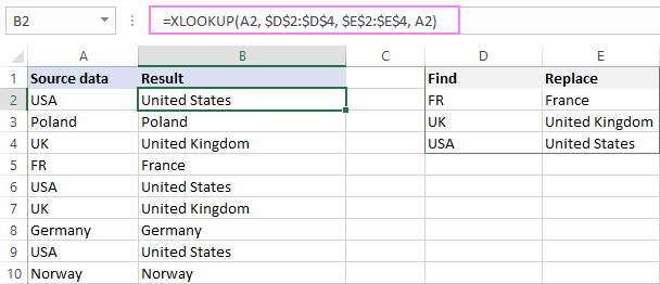
Since the XLOOKUP function is only available in Excel 365, the above formula won’t work in earlier versions. However, you can easily mimic this behavior with a combination of IFERROR or IFNA and VLOOKUP:
=IFNA(VLOOKUP(A2, $D$2:$E$4, 2, FALSE), A2) 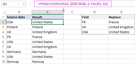
Note. Unlike SUBSTITUTE, the XLOOKUP and VLOOKUP functions are not case-sensitive, meaning they search for the lookup values ignoring the letter case. For instance, our formula would replace both FR and fr with France.
Advantages: unusual use of usual functions; works in all Excel versions
Drawbacks: works on a cell level, cannot replace part of the cell contents
Multiple replace using recursive LAMBDA function
For Microsoft 365 subscribers, Excel provides a special function that allows creating custom functions using a traditional formula language. Yep, I’m talking about LAMBDA. The beauty of this method is that it can convert a very lengthy and complex formula into a very compact and simple one. Moreover, it lets you create your own functions that do not exist in Excel, something that was before possible only with VBA.
For the detailed information about creating and using custom LAMBDA functions, please check out this tutorial: How to write LAMBDA functions in Excel. Here, we will discuss a couple of practical examples.
Advantages: the result is an elegant and amazingly simple to use function, no matter the number of replacement pairs
Drawbacks: available only in Excel 365; workbook-specific and cannot be reused across different workbooks
Example 1. Search and replace multiple words / strings at once
To replace multiple words or text in one go, we’ve created a custom LAMBDA function, named MultiReplace, which can take one of these forms:
=LAMBDA(text, old, new, IF(old<>«», MultiReplace(SUBSTITUTE(text, old, new), OFFSET(old, 1, 0), OFFSET(new, 1, 0)), text))
=LAMBDA(text, old, new, IF(old=»», text, MultiReplace(SUBSTITUTE(text, old, new), OFFSET(old, 1, 0), OFFSET(new, 1, 0))))
Both are recursive functions that call themselves. The difference is only in how the exit point is established.
In the first formula, the IF function checks whether the old list is not blank (old<>«»). If TRUE, the MultiReplace function is called. If FALSE, the function returns text it its current form and exits.
The second formula uses the reverse logic: if old is blank (old=»»), then return text and exit; otherwise call MultiReplace.
The trickiest part is accomplished! What is left for you to do is to name the MultiReplace function in the Name Manager like shown in the screenshot below. For the detailed guidelines, please see How to name a LAMBDA function. 
Once the function gets a name, you can use it just like any other inbuilt function.
Whichever of the two formula variations you choose, from the end-user perspective, the syntax is as simple as this:
- Text — the source data
- Old — the values to find
- New — the values to replace with
Taking the previous example a little further, let’s replace not only the country abbreviations but the state abbreviations as well. For this, type the abbreviations (old values) in column D beginning in D2 and the full names (new values) in column E beginning in E2.
In B2, enter the MultiReplace function:
=MultiReplace(A2:A10, D2, E2)
Hit Enter and enjoy the results 🙂 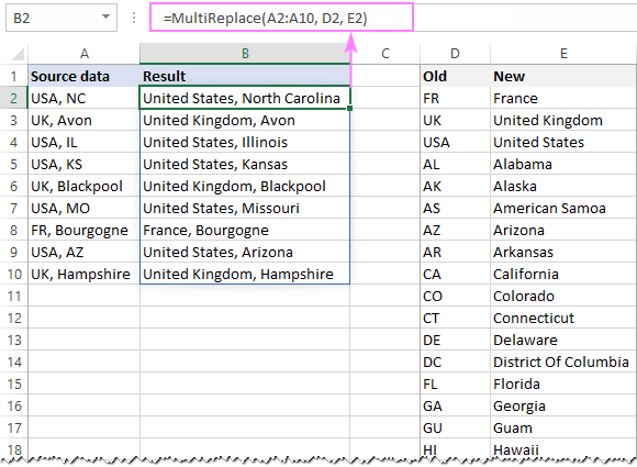
How this formula works
The clue to understanding the formula is understanding recursion. This may sound complicated, but the principle is quite simple. With each iteration, a recursive function solves one small instance of a bigger problem. In our case, the MultiReplace function loops through the old and new values and, with each loop, performs one replacement:
MultiReplace (SUBSTITUTE(text, old, new), OFFSET(old, 1, 0), OFFSET(new, 1, 0))
As with nested SUBSTITUTE functions, the result of the previous SUBSTITUTE becomes the text parameter for the next SUBSTITUTE. In other words, on each subsequent call of MultiReplace, the SUBSTITUTE function processes not the original text string, but the output of the previous call.
To handle all the items on the old list, we start with the topmost cell, and use the OFFSET function to move 1 row down with each interaction:
The same is done for the new list:
The crucial thing is to provide a point of exit to prevent recursive calls from proceeding forever. It is done with the help of the IF function — if the old cell is empty, the function returns text it its present form and exits:
=LAMBDA(text, old, new, IF(old=»», text, MultiReplace(…)))
=LAMBDA(text, old, new, IF(old<>«», MultiReplace(…), text))
Example 2. Replace multiple characters in Excel
In principle, the MultiReplace function discussed in the previous example can handle individual characters as well, provided that each old and new character is entered in a separate cell, exactly like the abbreviated and full names in the above screenshots.
If you’d rather input the old characters in one cell and the new characters in another cell, or type them directly in the formula, then you can create another custom function, named ReplaceChars, by using one of these formulas:
=LAMBDA(text, old_chars, new_chars, IF(old_chars<>«», ReplaceChars(SUBSTITUTE(text, LEFT(old_chars), LEFT(new_chars)), RIGHT(old_chars, LEN(old_chars)-1), RIGHT(new_chars, LEN(new_chars)-1)), text))
=LAMBDA(text, old_chars, new_chars, IF(old_chars=»», text, ReplaceChars(SUBSTITUTE(text, LEFT(old_chars), LEFT(new_chars)), RIGHT(old_chars, LEN(old_chars)-1), RIGHT(new_chars, LEN(new_chars)-1))))
Remember to name your new Lambda function in the Name Manager as usual: 
And your new custom function is ready for use:
- Text — the original strings
- Old — the characters to search for
- New — the characters to replace with
To give it a field test, let’s do something that is often performed on imported data — replace smart quotes and smart apostrophes with straight quotes and straight apostrophes.
First, we input the smart quotes and smart apostrophe in D2, straight quotes and straight apostrophe in E2, separating the characters with spaces for better readability. (As we use the same delimiter in both cells, it won’t have any impact on the result — Excel will just replace a space with a space.)
After that, we enter this formula in B2:
=ReplaceChars(A2:A4, D2, E2)
And get exactly the results we were looking for: 
It is also possible to type the characters directly in the formula. In our case, just remember to «duplicate» the straight quotes like this:
=ReplaceChars(A2:A4, «вЂњ ” ’», «»» «» ‘»)
How this formula works
The ReplaceChars function cycles through the old_chars and new_chars strings and makes one replacement at a time beginning from the first character on the left. This part is done by the SUBSTITUTE function:
SUBSTITUTE(text, LEFT(old_chars), LEFT(new_chars))
With each iteration, the RIGHT function strips off one character from the left of both the old_chars and new_chars strings, so that LEFT could fetch the next pair of characters for substitution:
ReplaceChars(SUBSTITUTE(text, LEFT(old_chars), LEFT(new_chars)), RIGHT(old_chars, LEN(old_chars)-1), RIGHT(new_chars, LEN(new_chars)-1))
Before each recursive call, the IF function evaluates the old_chars string. If it is not empty, the function calls itself. As soon as the last character has been replaced, the iteration process finishes, the formula returns text it its present form and exits.
Note. Because the SUBSTITUTE function used in our core formulas is case-sensitive, both Lambdas (MultiReplace and ReplaceChars) treat uppercase and lowercase letters as different characters.
Mass find and replace with UDF
In case the LAMBDA function is not available in your Excel, you can write a user-defined function for multi-replace in a traditional way using VBA.
To distinguish the UDF from the LAMBDA-defined MultiReplace function, we are going to name it differently, say MassReplace. The code of the function is as follows:
Like LAMBDA-defined functions, UDFs are workbook-wide. That means the MassReplace function will work only in the workbook in which you have inserted the code. If you are not sure how to do this correctly, please follow the steps described in How to insert VBA code in Excel.
Once the code is added to your workbook, the function will appear in the formula intellisense — only the function’s name, not the arguments! Though, I believe it’s no big deal to remember the syntax:
- Input_range — the source range where you want to replace values.
- Find_range — the characters, strings, or words to search for.
- Replace_range — the characters, strings, or words to replace with.
In Excel 365, due to support for dynamic arrays, this works as a normal formula, which only needs to be entered in the top cell (B2):
=MassReplace(A2:A10, D2:D4, E2:E4) 
In pre-dynamic Excel, this works as an old-style CSE array formula: you select the entire source range (B2:B10), type the formula, and press the Ctrl + Shift + Enter keys simultaneously to complete it. 
Advantages: a decent alternative to a custom LAMBDA function in Excel 2019, Excel 2016 and earlier versions
Drawbacks: the workbook must be saved as a macro-enabled .xlsm file
Bulk replace in Excel with VBA macro
If you love automating common tasks with macros, then you can use the following VBA code to find and replace multiple values in a range.
To make use of the macro right away, you can download our sample workbook containing the code. Or you can insert the code in your own workbook.
How to use the macro
Before running the macro, type the old and new values into two adjacent columns as shown in the image below (C2:D4).
And then, select your source data, press Alt + F8 , pick the BulkReplace macro, and click Run. 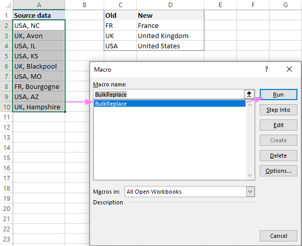
As the source rage is preselected, just verify the reference, and click OK: 
After that, select the replace range, and click OK: 
Done! 
Advantages: setup once, re-use anytime
Drawbacks: the macro needs to be run with every data change
Multiple find and replace in Excel with Substring tool
In the very first example, I mentioned that nested SUBSTITUTE is the easiest way to replace multiple values in Excel. I admit that I was wrong. Our Ultimate Suite makes things even easier!
To do mass replace in your worksheet, head over to the Ablebits Data tab and click Substring Tools > Replace Substrings. 
The Replace Substrings dialog box will appear asking you to define the Source range and Substrings range. 
With the two ranges selected, click the Replace button and find the results in a new column inserted to the right of the original data. Yep, it’s that easy! 
Tip. Before clicking Replace, there is one important thing for you to consider — the Case-sensitive box. Be sure to select it if you wish to handle the uppercase and lowercase letters as different characters. In this example, we tick this option because we only want to replace the capitalized strings and leave the substrings like «fr», «uk», or «ak» within other words intact.
If you are curious to know what other bulk operations can be performed on strings, check out other Substring Tools included with our Ultimate Suite. Or even better, download the evaluation version below and give it a try!
That’s how to find and replace multiple words and characters at once in Excel. I thank you for reading and hope to see you on our blog next week!
Источник
REPLACE function is included in the text functions of MS Excel and is intended to replace a specific area of the text string containing the source text on the specified text line (new text).
How does the REPLACE function in Excel work?
Example 1. In order to study in detail the operation of this function, we consider one of the simplest examples. Suppose we have several words in different columns, we need to get new words using the original ones. For this example, in addition to our main function REPLACE, we also use the RIGHT function — this function serves to return a certain number of characters from the end of a line of text. That is, for example, we have two words: milk and a skating rink, as a result we must get the word hammer.
REPLACE function in Excel and examples of its use
- Create a table with words on the sheet of the Excel spreadsheet workbook, as shown in the figure:
- Next, on the sheet of the workbook, we will prepare an area for placing our result — the resulting word “hammer”, as shown below. Place the cursor in cell A6 and call the function REPLACE:
- Fill the function with the arguments shown in the figure:
Let us explain the choice of these parameters as follows: cell A2 was chosen as the beginning of the text, the number 5 was set as beginning_, since it is from the fifth position of the word “Milk” we don’t take characters for our final word, the number_ of signs was set equal to 2, since this number It is not taken into account in the new word, as the new text, the set option RIGHT with the parameters of the cell A3 and taking the last two characters «ok».
Next, click on the «OK» button and get the result:
How to REPLACE a piece of text in Excel cell?
Example 2. Consider another small example. Suppose we have columns of words in the cells of the Excel spreadsheet. It is necessary to replace their letters in certain places so as to convert them.
- Let’s create a tablet with words on the sheet of an Excel workbook, as shown in the figure:
- Further, on the same sheet of the working book we will prepare an area for placing our result — modified words. Fill the cells with two types of formulas as shown in the picture:
Download examples text function REPLACE in Excel
Note! In the second formula, we use the operator “&” to add the character «s» to the male surname to convert it to the female. To solve this problem, one could use the function =CONCATENATE(B3,»s») instead of the formula =B3&»s» — the result is identical. But today it is strongly recommended to abandon this formula as it has its limitations and is more demanding on resources in comparison with a simple and convenient ampersand operator.