
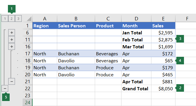
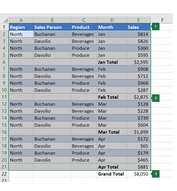
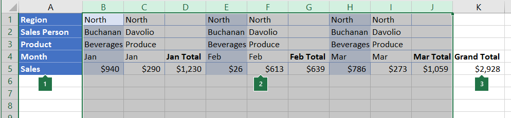
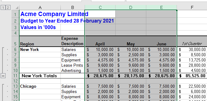
If you have a list of data you want to group and summarize, you can create an outline of up to eight levels. Each inner level, represented by a higher number in the outline symbols, displays detail data for the preceding outer level, represented by a lower number in the outline symbols. Use an outline to quickly display summary rows or columns, or to reveal the detail data for each group. You can create an outline of rows (as shown in the example below), an outline of columns, or an outline of both rows and columns.
|
|
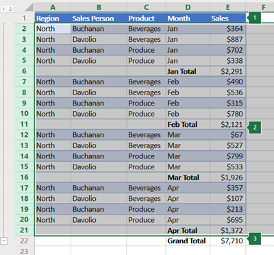
1. To display rows for a level, click the appropriate 2. Level 1 contains the total sales for all detail rows. 3. Level 2 contains total sales for each month in each region. 4. Level 3 contains detail rows — in this case, rows 17 through 20. 5. To expand or collapse data in your outline, click the |
 outline symbols.
 and
and  outline symbols, or press ALT+SHIFT+= to expand and ALT+SHIFT+- to collapse.
-
Make sure that each column of the data that you want to outline has a label in the first row (e.g., Region), contains similar facts in each column, and that the range you want to outline has no blank rows or columns.
-
If you want, your grouped detail rows can have a corresponding summary row—a subtotal. To create these, do one of the following:
-
Insert summary rows by using the Subtotal command
Use the Subtotal command, which inserts the SUBTOTAL function immediately below or above each group of detail rows and automatically creates the outline for you. For more information about using the Subtotal function, see SUBTOTAL function.
-
Insert your own summary rows
Insert your own summary rows, with formulas, immediately below or above each group of detail rows. For example, under (or above) the rows of sales data for March and April, use the SUM function to subtotal the sales for those months. The table later in this topic shows you an example of this.
-
-
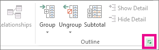
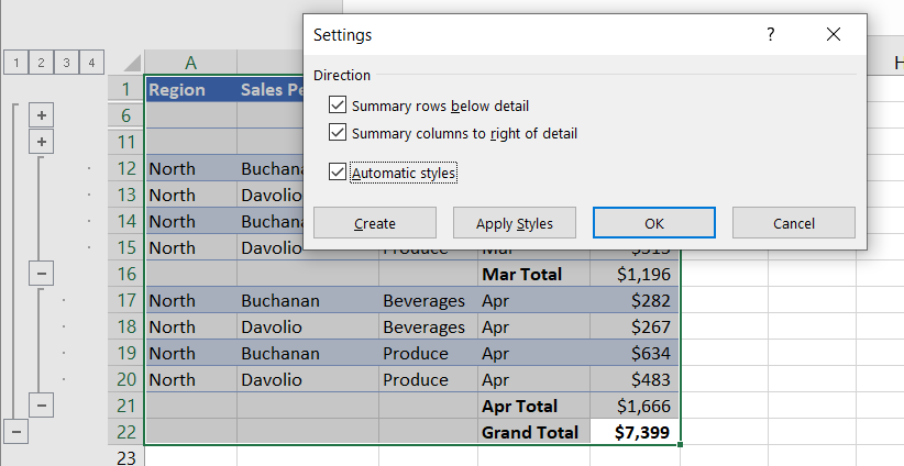
By default, Excel looks for summary rows below the details they summarize, but it’s possible to create them above the detail rows. If you created the summary rows below the details, skip to the next step (step 4). If you created your summary rows above your detail rows, on the Data tab, in the Outline group, click the dialog box launcher.

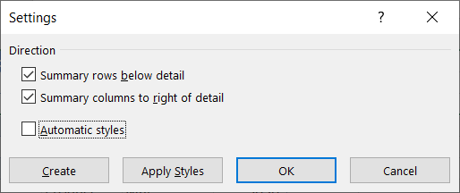
The Settings dialog box opens.
Then in the Settings dialog box, clear the Summary rows below detail checkbox, and then click OK.
-
Outline your data. Do one of the following:
Outline the data automatically
-
Select a cell in the range of cells you want to outline.
-
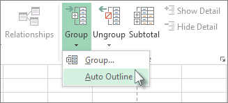
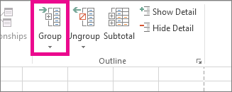
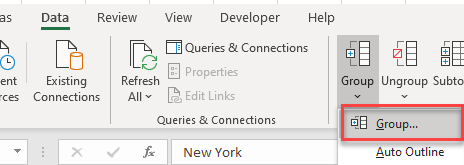
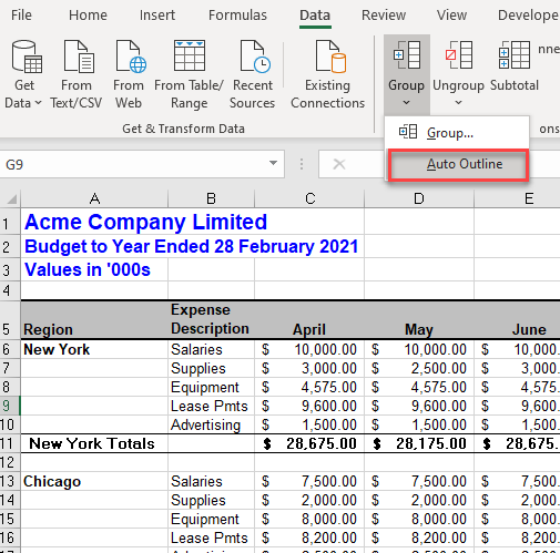
On the Data tab, in the Outline group, click the arrow under Group, and then click Auto Outline.
Outline the data manually
Important: When you manually group outline levels, it’s best to have all data displayed to avoid grouping the rows incorrectly.
-
To outline the outer group (level 1), select all of the rows the outer group will contain (i.e., the detail rows and if you added them, their summary rows).
1. The first row contains labels, and is not selected.
2. Since this is the outer group, select all the rows with subtotals and details.
3. Don’t select the grand total.
-
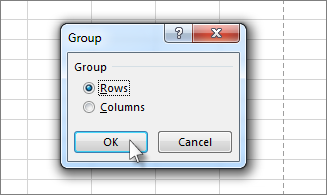
On the Data tab, in the Outline group, click Group. Then in the Group dialog box, click Rows, and then click OK.
Tip: If you select entire rows instead of just the cells, Excel automatically groups by row — the Group dialog box doesn’t even open.
The outline symbols appear beside the group on the screen.
-
Optionally, outline an inner, nested group — the detail rows for a given section of your data.
Note: If you don’t need to create any inner groups, skip to step f, below.
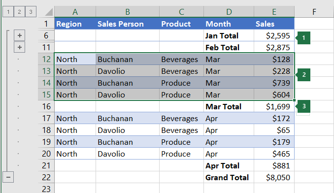
For each inner, nested group, select the detail rows adjacent to the row that contains the summary row.
1. You can create multiple groups at each inner level. Here, two sections are already grouped at level 2.
2. This section is selected and ready to group.
3. Don’t select the summary row for the data you are grouping.
-
On the Data tab, in the Outline group, click Group.
Then in the Group dialog box, click Rows, and then click OK. The outline symbols appear beside the group on the screen.
Tip: If you select entire rows instead of just the cells, Excel automatically groups by row — the Group dialog box doesn’t even open.
-
Continue selecting and grouping inner rows until you have created all of the levels that you want in the outline.
-
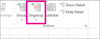
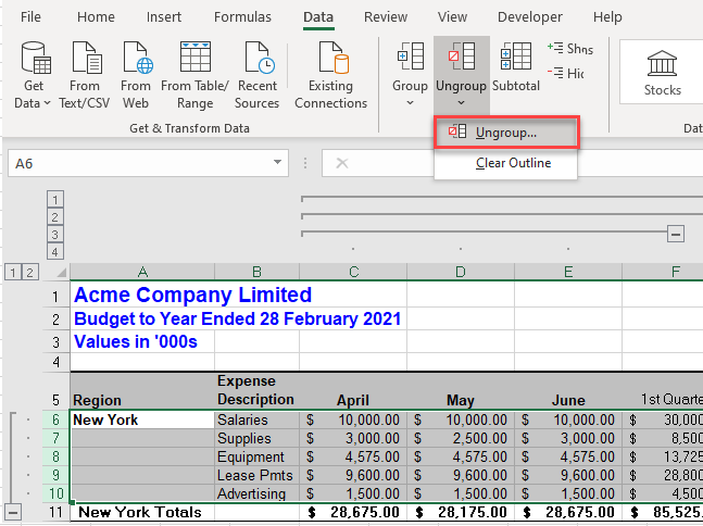
If you want to ungroup rows, select the rows, and then on the Data tab, in the Outline group, click Ungroup.
You can also ungroup sections of the outline without removing the entire level. Hold down SHIFT while you click the
or for the group, and then on the Data tab, in the Outline group, click Ungroup.Important: If you ungroup an outline while the detail data is hidden, the detail rows may remain hidden. To display the data, drag across the visible row numbers adjacent to the hidden rows. Then on the Home tab, in the Cells group, click Format, point to Hide & Unhide, and then click Unhide Rows.
-
-
Make sure that each row of the data that you want to outline has a label in the first column, contains similar facts in each row, and the range has no blank rows or columns.
-
Insert your own summary columns with formulas immediately to the right or left of each group of detail columns. The table listed in step 4 below shows you an example.
Note: To outline data by columns, you must have summary columns that contain formulas that reference cells in each of the detail columns for that group.
-
If your summary column is to the left of the detail columns, on the Data tab, in the Outline group, click the dialog box launcher.
The Settings dialog box opens.
Then in the Settings dialog box, clear the Summary columns to right of detail check box, and click OK.
-
To outline the data, do one of the following:
Outline the data automatically
-
Select a cell in the range.
-
On the Data tab, in the Outline group, click the arrow below Group and click Auto Outline.
Outline the data manually
Important: When you manually group outline levels, it’s best to have all data displayed to avoid grouping columns incorrectly.
-
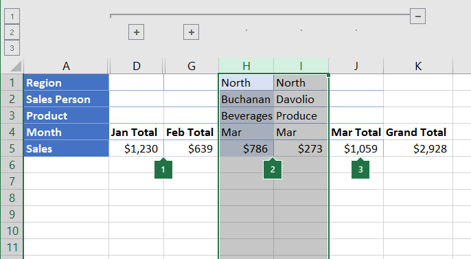
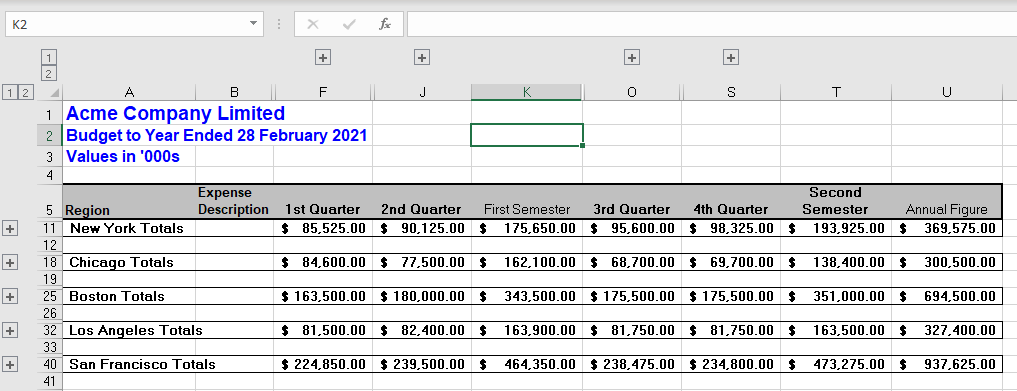
To outline the outer group (level 1), select all of the subordinate summary columns, as well as their related detail data.
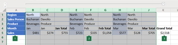
1. Column A contains labels.
2. Select all the detail and subtotal columns. Note that if you don’t select entire columns, when you click Group (on the Data tab in the Outline group) the Group dialog box will open and ask you to choose Rows or Columns.
3. Don’t select the grand total column.
-
On the Data tab, in the Outline group, click Group.
The outline symbol appears above the group.
-
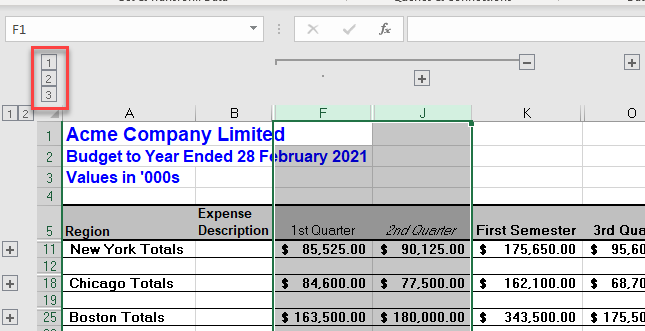
To outline an inner, nested group of detail columns (level 2 or higher), select the detail columns adjacent to the column that contains the summary column.
1. You can create multiple groups at each inner level. Here, two sections are already grouped at level 2.
2. These columns are selected and ready to group. Note that if you don’t select entire columns, when you click Group (on the Data tab in the Outline group) the Group dialog box will open and ask you to choose Rows or Columns.
3. Don’t select the summary column for the data you are grouping.
-
On the Data tab, in the Outline group, click Group.
The outline symbols appear beside the group on the screen.
-
-
Continue selecting and grouping inner columns until you have created all of the levels that you want in the outline.
-
If you want to ungroup columns, select the columns, and then on the Data tab, in the Outline group, click Ungroup.
You can also ungroup sections of the outline without removing the entire level. Hold down SHIFT while you click the  or
or  for the group, and then on the Data tab, in the Outline group, click Ungroup.
If you ungroup an outline while the detail data is hidden, the detail columns may remain hidden. To display the data, drag across the visible column letters adjacent to the hidden columns. On the Home tab, in the Cells group, click Format, point to Hide & Unhide, and then click Unhide Columns
-
If you don’t see the outline symbols
, , and , go to File > Options > Advanced, and then under the Display options for this worksheet section, select the Show outline symbols if an outline is applied check box, and then click OK. -
Do one or more of the following:
-
Show or hide the detail data for a group
To display the detail data within a group, click the
button for the group, or press ALT+SHIFT+=. -
To hide the detail data for a group, click the
button for the group, or press ALT+SHIFT+-. -
Expand or collapse the entire outline to a particular level
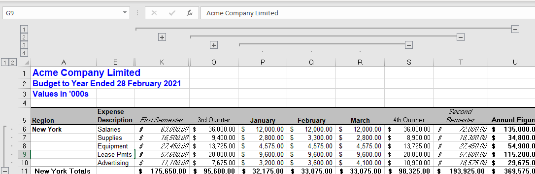
In the
outline symbols, click the number of the level that you want. Detail data at lower levels is then hidden.For example, if an outline has four levels, you can hide the fourth level while displaying the rest of the levels by clicking
. -
Show or hide all of the outlined detail data
To show all detail data, click the lowest level in the
outline symbols. For example, if there are three levels, click . -
To hide all detail data, click
.
-
 .
. .
.For outlined rows, Microsoft Excel uses styles such as RowLevel_1 and RowLevel_2 . For outlined columns, Excel uses styles such as ColLevel_1 and ColLevel_2. These styles use bold, italic, and other text formats to differentiate the summary rows or columns in your data. By changing the way each of these styles is defined, you can apply different text and cell formats to customize the appearance of your outline. You can apply a style to an outline either when you create the outline or after you create it.
Do one or more of the following:
Automatically apply a style to new summary rows or columns
-
On the Data tab, in the Outline group, click the dialog box launcher.
The Settings dialog box opens.
-
Select the Automatic styles check box.
Apply a style to an existing summary row or column
-
Select the cells to which you want to apply a style.
-
On the Data tab, in the Outline group, click the dialog box launcher.
The Settings dialog box opens.
-
Select the Automatic styles check box, and then click Apply Styles.
You can also use autoformats to format outlined data.
-
If you don’t see the outline symbols
, , and , go to File > Options > Advanced, and then under the Display options for this worksheet section, select the Show outline symbols if an outline is applied check box. -
Use the outline symbols
, , and to hide the detail data that you don’t want copied.For more information, see the section, Show or hide outlined data.
-
Select the range of summary rows.
-
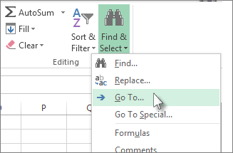
On the Home tab, in the Editing group, click Find & Select, and then click Go To.
-
Click Go To Special.
-
Click Visible cells only.
-
Click OK, and then copy the data.
Note: No data is deleted when you hide or remove an outline.
Hide an outline
-
Go to File > Options > Advanced, and then under the Display options for this worksheet section, uncheck the Show outline symbols if an outline is applied check box.
Remove an outline
-
Click the worksheet.
-
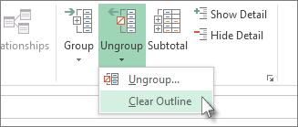
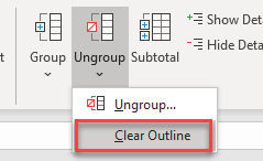
One the Data tab, in the Outline group, click Ungroup and click Clear Outline.
Important: If you remove an outline while the detail data is hidden, the detail rows or columns may remain hidden. To display the data, drag across the visible row numbers or column letters adjacent to the hidden rows and columns. On the Home tab, in the Cells group, click Format, point to Hide & Unhide, and then click Unhide Rows or Unhide Columns.
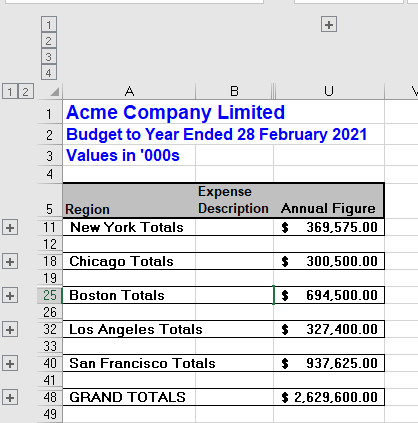
Imagine that you want to create a summary report of your data that only displays totals accompanied by a chart of those totals. In general, you can do the following:
-
Create a summary report
-
Outline your data.
For more information, see the sections Create an outline of rows or Create an outline of columns.
-
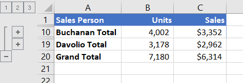
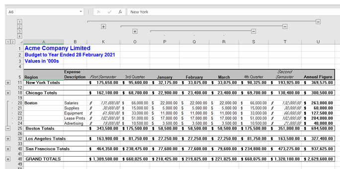
Hide the detail by clicking the outline symbols
, , and to show only the totals as shown in the following example of a row outline:
-
For more information, see the section, Show or hide outlined data.
-
-
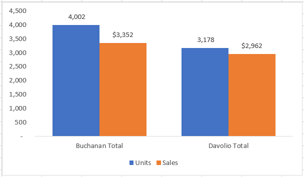
Chart the summary report
-
Select the summary data that you want to chart.
For example, to chart only the Buchanan and Davolio totals, but not the grand totals, select cells A1 through C19 as shown in the above example.
-
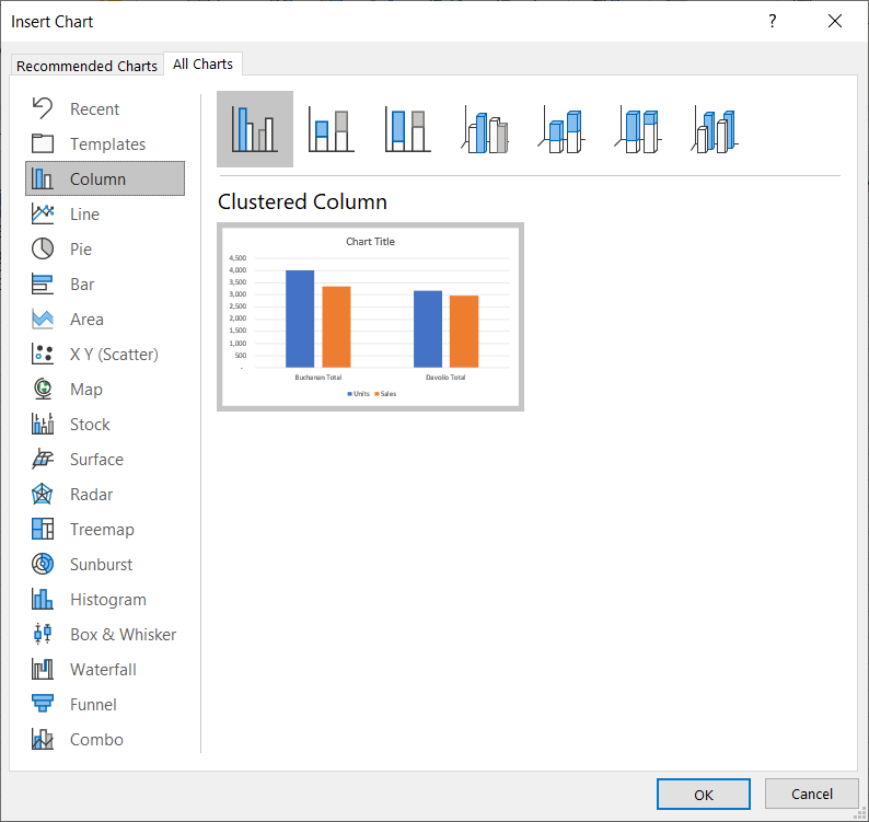
Click Insert > Charts > Recommended Charts, then click the All Charts tab and choose your chart type.
For example, if you chose the Clustered Column option, your chart would look like this:
If you show or hide details in the outlined list of data, the chart is also updated to show or hide the data.
-
You can group (or outline) rows and columns in Excel for the web.
Note: Although you can add summary rows or columns to your data (by using functions such as SUM or SUBTOTAL), you cannot apply styles or set a position for summary rows and columns in Excel for the web.
Create an outline of rows or columns
|
|
|
|
Outline of rows in Excel Online
|
Outline of columns in Excel Online
|
-
Make sure that each column (or row) of the data that you want to outline has a label in the first row (or column), contains similar facts in each column (or row), and that the range has no blank rows or columns.
-
Select the data (including any summary rows or columns).
-
On the Data tab, in the Outline group, click Group > Group Rows or Group Columns.
-
Optionally, if you want to outline an inner, nested group — select the rows or columns within the outlined data range, and repeat step 3.
-
Continue selecting and grouping inner rows or columns until you have created all of the levels that you want in the outline.
Ungroup rows or columns
-
To ungroup, select the rows or columns, and then on the Data tab, in the Outline group, click Ungroup and select Ungroup Rows or Ungroup Columns.
Show or hide outlined data
Do one or more of the following:
Show or hide the detail data for a group
-
To display the detail data within a group, click the
for the group, or press ALT+SHIFT+=. -
To hide the detail data for a group, click the
for the group, or press ALT+SHIFT+-.
Expand or collapse the entire outline to a particular level
-
In the
outline symbols, click the number of the level that you want. Detail data at lower levels is then hidden. -
For example, if an outline has four levels, you can hide the fourth level while displaying the rest of the levels by clicking
.
Show or hide all of the outlined detail data
-
To show all detail data, click the lowest level in the
outline symbols. For example, if there are three levels, click . -
To hide all detail data, click
.
Need more help?
You can always ask an expert in the Excel Tech Community or get support in the Answers community.
See Also
Group or ungroup data in a PivotTable
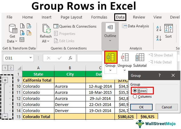
Grouping Rows in Excel
In Excel, organizing the large data by combining the subcategory data is called “grouping of rows.” When the number of items in line is not important, we can choose group rows that are not important but only see the subtotal of those rows. On the other hand, when the data rows are huge, scrolling down and reading the report may lead to a wrong understanding, so the grouping of rows helps us hide the unwanted numbers of rows.
The number of rows is also lengthy when the worksheet contains detailed information or data. However, report readers of the data do not want to see long rows. Instead, they want to see a clear view, but at the same time, if they require any other detailed information, they need just a button to expand or collapse them as needed.
This article will show you how to group rows in Excel with expand/collapse to maximize the report viewing technique.
Table of contents
- Grouping Rows in Excel
- How to Group Rows in Excel with Expand/Collapse?
- Group by Using Shortcut Key
- Example #1 – Using Auto Outline
- Example #2 – Using Subtotals
- Things to Remember here
- Recommended Articles
- How to Group Rows in Excel with Expand/Collapse?
How to Group Rows in Excel with Expand/Collapse?
You can download this Group Rows Excel Template here – Group Rows Excel Template
For example, look at the below data.
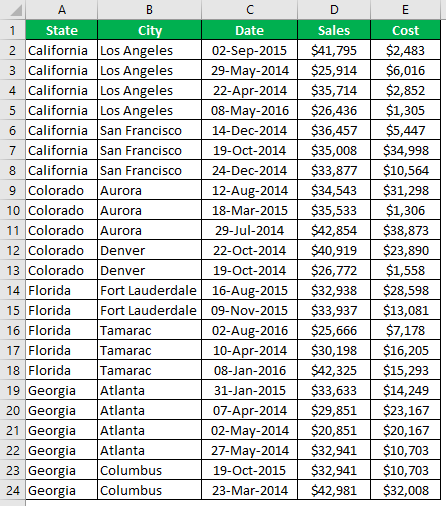
We have city and state-related sales and cost data in the table above. Still, when we look at the first two rows of the data, we have “California” state and the city is “Los Angeles,” but sales happened on different dates. Hence, as a report reader, everyone prefers to read the state-wise sales and city-wise sales in a single column, so we can create a single line summary view by grouping the rows.
Follow the below steps to group rows in excel.
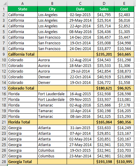
- First, we must create a subtotal like the one below.

- We must select the first state rows (California state), excluding subtotals.

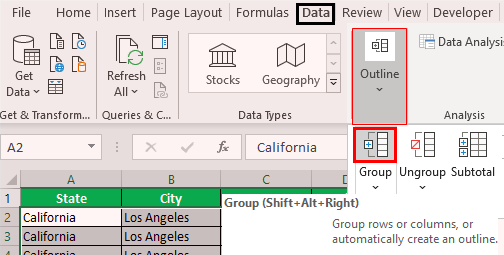
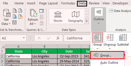
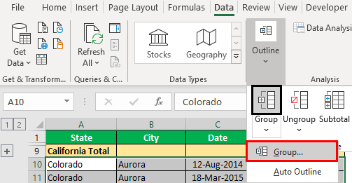
- Then, go to the Data tab and choose the “Group” option.

- Click on the drop-down list in excel of “Group” and choose “Group” again.
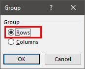
- Now, it may ask whether to group rows or columns. Since we are grouping Rows, we must choose Rows and click on OK.

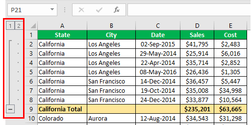
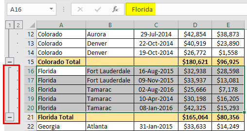
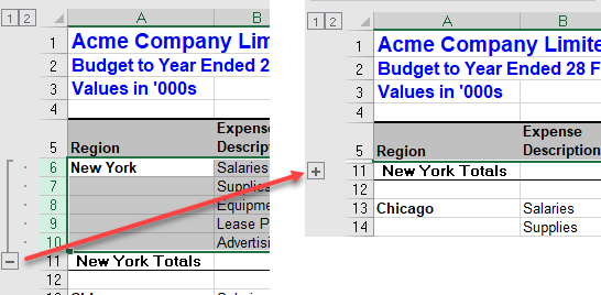
- The moment we click on OK, we can see a joint line on the left-hand side.

- Then, we must click on the minus icon and see the magic.

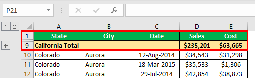
Now, we can see the total summary for the city California. Again, if we want to see a detailed overview of the city, we can click on the plus icon to expand the view. - Now again, select the city Colorado and click on the Group option.

- As a result, it will group for the Colorado state.


Group by Using Shortcut Key
With a simple shortcut in excelAn Excel shortcut is a technique of performing a manual task in a quicker way.read more, we can easily group selected rows or columns. The shortcut key to group the data is “SHIFT + ALT + Right Arrow key.”
![]()
First, we must select the rows that need to be grouped.

To group these rows, we must press the shortcut key “SHIFT + ALT + Right Arrow key.“
In the above, we have seen how to group the data and row with expanding and collapse options using the “PLUS” and “MINUS” icons.
The only problem with the above method is that we need to do this for each state individually, so this takes a lot of time when there are many states. So, what would be your reaction if we say you can group with just one click?
Amazing. Using the “Auto Outline,” we can automatically group the data.
Example #1 – Using Auto Outline
First we need to create subtotal rows.

Now, we must place a cursor inside the data range. Under the “Group” drop-down, we can see one more option other than “Group,” which is “Auto Outline.”

The moment we click on this “Auto Outline” option, it will group all the rows above the subtotal row.

How cool is this??? Very cool, isn’t it??
Example #2 – Using Subtotals
If grouping the rows for the individual city is the one problem, then even before grouping rows, there is another problem: adding subtotal rows.
When there are hundreds of states, it is a tough task to create a subtotal row for each state separately, so we can use the “Subtotal” option to create a subtotal for the selected column quickly.
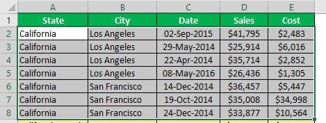
For example, we had the data like the below before creating the subtotal.

Under the “Data” tab, we have an option called “Subtotal” right next to the “Group” option.

Click on this option by selecting any of the cells of the data range. It will show the below option first up.

First, select the column that needs a subtotal. In this example, we need subtotal for “State,” so choose the same from the drop-down list of “At each change in.”

Next, we need to select the function type since we add all the values to choose “Sum” function in excel.

Now, select the columns that need to be summed. We need the summary of the “Sales“and “Cost” columns, so choose the same. Click on “OK.”

We will have subtotal rows shortly.

Did you notice one special thing from the above image???
It has automatically grouped rows for us!!!!
Things to Remember here
- The shortcut key for grouping rows is the “Shift + ALT + Right Arrow” key.
- We should sort subtotal that needs data.
- The “Auto Outline” option can group all the rows above the subtotal row.
Recommended Articles
This article is a guide to Group Rows in Excel. We discuss grouping rows in Excel with expand/collapse using an auto outline and subtotal options with examples and a downloadable Excel template. You may also look at these useful functions in Excel: –
- Excel Maximum Number of Rows
- Divide Cell in ExcelDivide in Excel is used for division applications, where (/) is the symbol and we can write an expression =a/b, where a and b represent two numbers or values to be divided.read more
- Group Columns in ExcelIn Excel, grouping one or more columns together in a worksheet is referred to as group column and I t allows you to contract or expand the column.read more
- Group Worksheets In ExcelGrouping gives the best results to users when the same type of data is presented in the cells of the same addresses. Grouping also improves the accuracy of data and eliminates the error made by a human in performing the calculations.read more
Many Excel users often work with large datasets in Excel. And large datasets are often split into different categories row-wise.
In such cases, it would become difficult to get an overview of the categories. One thing that would help would be to group similar items under each category to better organize the data.
Excel provides us with the functionality to group rows so that we may organize data in a better way.
The grouped rows may be collapsed or expanded as required.
Take a look at the dataset below.

The dataset shows items sold by different representatives in different regions.
For large datasets, it may be helpful to organize the regions in groups so that we may have an idea of how many regions there are.
Also, we may want to see the total sale made in a particular region without seeing the individual entries.
So in this tutorial, I will show you different methods by which you can group rows in Excel.
Method 1: Group Rows in Excel Using the Group Option
In this method, we will look at the ‘Group Rows’ option in the ribbon in Excel to group rows containing similar data.
As an example, we will use the following dataset that we saw earlier. Here we will group all the rows for the Central region.

- Select all rows containing the Central region. These are rows 2 to 8.

- Go to the Data tab.

- Under the Data tab, click on the Group button.

- All the rows containing the Central region will be grouped. This is evident from the line and minus sign that appears on the left side of the worksheet area (as shown below).

- Click on the Minus sign to collapse all the rows.

- The result will be as shown.

As you can see that the grouped rows have collapsed, and the minus sign will change to a plus.
- Click on the Plus sign to expand all the grouped rows. The result will be as shown.

So in this method, we have seen how to group rows and collapse and expand them as we like.
Note: When we use this method to group rows in Excel, all the group rows would be held when you collapse the group. this would be useful in situations where you have multiple groups, and you want to only focus on showing some of the groups while hiding the rest
Method 2: Group Rows in Excel Using Keyboard Shortcut
In this method, we will look at the keyboard shortcut keys to group rows containing similar data.
As an example, we will use the dataset used in the previous method. Here we will group all the rows for the Central region.
- Select all rows containing the Central region. These are rows 2 to 8.

- On your keyboard, press Shift + Alt + Right Arrow.
- You will see that all rows containing the Central region will be grouped. This is evident from the line and minus sign shown.

So in this method, we have seen how to group rows using a keyboard shortcut.
As with the previous method, you can collapse or expand the grouped rows using the minus or plus signs respectively.
Method 3: Group Rows in Excel Using the Auto Outline Option
In this method, we will look at the Auto Outline option to group rows.
As an example, we will use the dataset as we did in previous methods.
However, to use Auto Outline, we will have to modify the dataset slightly.
We will have to insert additional rows that will differentiate between the groups. The dataset will be as shown.

Here I have added three additional rows, as shown. In each of these rows, I have also calculated the total sale made in each region.
- Go to the Data tab.

- Click on the arrow next to the Group button.

- The following dropdown menu will appear.

- From this menu, select the Auto Outline option.

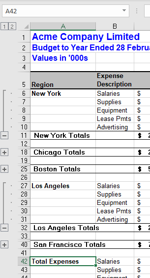
- You will see that all the different regions have been grouped. Note the minus sign appearing before each.

- Click on all minus signs to collapse all grouped rows.

- The result will look like the one below.

As you can see, the rows have collapsed, and we can now see the total for each region without seeing the individual entries.
Note: For this method to work, you need to insert a new row in between the groups and also ensure that there is at least one column that has the sum of all the values in that column (for the rows that you need to group)
Method 4: Group Rows in Excel Using the Subtotal Option
In this method, we will use the Subtotal option to group rows.
The Subtotal option will not only group the rows, but will also provide a summary of the grouped data.
In the previous method, we had to create this summary by inserting additional rows and manually calculating the total sale made in each region.
The Subtotal option will insert the additional rows for us automatically and calculate the sum of the total sale made in each region.
We will use the same dataset as we did in the first method.

- Select the entire dataset as shown. This will be from cell A1 to cell G13.

- Go to the Data tab.

- Under the Data tab, select the Subtotal option.

- The Subtotal window will appear as shown.

- Under the ‘At each change in’ option, select Region. (This is the criteria on which we want to group our rows.

- Under the ‘Use function’ option, select Sum. (This is the operation we want to perform on the data.)

- Under the ‘Add subtotal to’ section, check the Total option. Uncheck all other options. (This is the data on which we want to perform the sum function we selected in the previous step)

- Check the ‘Replace current subtotals’ and ‘Summary below data’ options. Make sure that the ‘Page break between groups’ option is unchecked.

- Click on OK.

- The result will look like the one below. (Note the line and minus sign before each row group)

- Click on the three minus signs as shown.

- The end result will look as shown.

You can see that all the grouped rows have collapsed.
This summary of data is similar to the one we saw in the previous method.
So in this method, we have seen how to group rows and create a data summary simultaneously.
In this tutorial, I have shown different methods as to how you can group rows.
The first two methods group rows that are manually selected. Use these methods if you want to group some rows selectively.
Method 3 groups rows together but requires that the row groups be differentiated from each other. If your dataset is small and inserting new rows under each row group is not a problem, then Method 3 is very useful.
Method 4 is a fully automatic method where not only are rows grouped based on a given criterion, but the data is also summarized as per the selected function.
If your dataset is large and inserting new rows or calculating subtotals is cumbersome, go with Method 4.
Other Excel articles you may also like:
- How to Group and Ungroup Worksheets in Excel
- How to Group by Months in Excel Pivot Table?
- How to Swap Columns in Excel?
- How to Print Row Numbers in Excel
- Delete Blank Rows in Excel (5 Ways + VBA)
Piles upon piles of data can quickly become overwhelming and Excel offers an equally quick solution to organize data and group it. Since deleting data can’t be an option most of the time, grouping data allows you to choose which data you want to see and which you want to temporarily stow away.
In addition to that, you can hide all the hundreds of small detail entries and have the totals or subtotals of groups of data on display. This will aid in quick analysis as you can get categorized summaries or focus on the core areas.
The same treatment can be done to columns but today we are focusing on grouping rows in Excel and this tutorial is going to center around the Outline group from the Data tab. By the end of it, you will know how to group rows with simply an outline or also with summarized data.
An outline is the grouping mechanism added in the row header area and it can have up to 8 levels – levels being the subgrouping of the categories in the dataset. There’s a stream of stuff to learn so out with the oars and…
Row row row your groups! (Group group group your rows to be more specific.)
 1")
Method #1 – Using Group Feature
What better to group rows in Excel than the Group feature. The Group feature groups rows or columns, clubbing the rows/columns of the selected cells so that they can be expanded or collapsed as a group. Used once, the Group feature bunches the selection into a single group. The implication is that every group will have to be made individually.
Conceptually, the reason you would want to group rows is to bunch up certain categories together. For that, optimally, the data should be sorted or arranged so the Group feature can appropriately club them together.
With the following steps, you will be able to use the Group feature to group rows in Excel:
- Select the cells of the rows in the datasets that you want to group.
- In the case example shown below, we are aiming to group rows 3 to 8 to club the Haircut/Trim category together. We don’t need to select B3 to D8 for that; we can select the rows from any one column.
- To create the group, click on the Group button in the Data tab’s Outline
 2")
- A small pop-up window will need you to confirm if you want to create the group for rows or columns.
- Make sure the Rows radio button is selected in the pop-up. Then click on the OK.
 3")
The rows of the selected cells will be grouped, and this is what it looks like:
 4")
You can see the change in the row header area with a brace ending in a minus sign with numbers in boxes above it. This is what an outline refers to and it has no effect on the face of the dataset. The numbers denote the levels in the outline.
Here, we have created a 2-level outline with the first level being the Haircut/Trim category, and the second level being the detail rows of the group. As a group, an outline containing up to 8 levels can be created.
Note: There is no hard and fast rule to creating a group as it doesn’t have to be made for a defined category. A group can be of any set of rows of your choice and is made based on whatever the cell selection is.
Collapsing and Expanding Grouped Rows
In the outline symbols, click on the minus sign of the group to collapse the rows.
 5")
The minus sign has changed to a plus sign (that can be used to expand the column back).
The collapsed group hides the rows from the worksheet and the row numbering shows a wedge between rows 2 and 9.
 6")
Use the plus sign to expand the rows again:
 7")
The Show Detail and Hide Detail buttons can be used to expand and collapse groups of rows. Select a cell from a group that you want to show or hide and use the Show Detail or Hide Detail button accordingly. This will also work for multiple cell selections and therefore multiple groups.
 8")
Creating More Groups
To create a group out of another set of rows, the same steps will have to be repeated after selecting the set of cells. Forming another group out of a range disjointed from the first one would be no issue.
But if you are to make another group from a consecutive range (in our case example, that would be B3 to B9 with the next category i.e. Blow out), you will have to add an empty row between the categories otherwise the groups will fuse into one group.
After separating the categories with an empty row, follow these steps to create another group of rows:
- Select the range corresponding to the rows that will be grouped.
- Using our case example, the next group we want to create is of the rows with the details of the Blow out category. For that, we have selected B10 to B13. Also note that the categories have now been split with an empty row.
- Next, select the Group button in the Data
 9")
- Click on the OK button of the pop-up window after selecting the Rows
 10")
The next group will be formed:
 11")
Similarly, you can great groups other sets of rows in the dataset, taking care that consecutive groups are separated by an empty row. However, each group will have to be made individually as the Group feature doesn’t work on multiple selections. Use the Group feature for individual groups.
If you want all the categories grouped separately you should explore the other options in the Outline group under the Data tab. The other features are discussed ahead in this guide.
Adding More Levels in Outline
Adding more levels to the outline would mean clubbing together further subsets in the main sets of the rows which creates inner or nested levels. Outer levels can also be added by clubbing broader categories. It is as simple as forming any other group and depends upon the cell selection.
And, as mentioned earlier, you may find that the categories that you want to group need sorting or should be presorted.
It’s okay if you have already started grouping. You can clear the groups with the Ungroup button (next to the Group button), sort all the categories, and then create groups.
As in our case example, using Sort & Filter, we have alphabetically sorted the Service column before arranging it and numerically sorted the Branch column.
We have already added the groups for the Service categories so let’s proceed with grouping a branch which will add an inner level in the outline.
- Select the cells of the subcategory that you aim to group.
 12")
- From the Data tab, use the Group button and then select the OK command in the pop-up window that confirms grouping for rows.
- From a 2-level outline, the grouping has changed to a 3-level outline with the first level groups for the Service category, the second for the Branch subcategory, and the third for the detail rows.
 13")
Groups don’t just work in forward levels but also in backward levels and you can create a group of rows of a larger category. In our case, we can add a group of all the hair-related categories. Just select the relevant cells i.e. B3 to B25 for us, apply the Group feature and an outer level will be formed.
In the example shot ahead, we have made a group for the Make-up category too:
 14")
Note: To avoid incorrect grouping of the rows, make sure there are no hidden rows or data on the worksheet.
Method #2 – Using Keyboard Shortcut
The very same Group feature can be applied using a keyboard shortcut instead of using the Group button on the Ribbon. Have the cells of the target rows selected and the keyboard shortcut will form the group by leading you to the small pop-up window. The complete keyboard shortcut is:
Shift + Alt + Right arrow + Enter
Shift + Alt + Right arrow keys will apply the Group feature and pop open the Group dialog box.
Enter key will select the OK button in the dialog box (given that the Rows option is selected by default).
Create a group of rows with this keyboard shortcut using the steps ahead:
- From the dataset, select the cells to be grouped.
- We are selecting B3 to B8 to group the Haircut/Trim category.
 15")
- Use this keyboard shortcut to trigger the Group feature: Shift + Alt + Right arrow keys
- The Group pop-up window will appear.
- Press the Enter key after confirming that the Rows option is selected.
 16")
Now the Group feature will be applied completely and will club together the rows of the selected cells:
 17")
Method #3 – Using Auto Outline Feature
Adding groups of rows manually is the smart way if you only require a few of them. Suppose you want the whole dataset or a significant consecutive part of the dataset bunched for the respective categories, you can opt for the Auto Outline feature. But with a condition.
Auto Outline requires summary rows (e.g. totals or averages of the bunch that you want grouped) to pick up on the data and form the outline. This means that Auto Outline won’t be able to work unless the intended groups have been split by adding an extra row with some form of a calculated summary of the group in that row.
The Auto Outline feature does not affect the dataset itself, it only adds the outline of the groups in the row header area (which, you will see later, is different from the Subtotal feature). See the steps to use Auto Outline using our case example where we have added rows at the point we want the groups to break and have also added subtotals in those rows within the Sales column.
The subtotals have been added using the SUM function and also boldened. Then you can proceed with the steps below to group the rows with Auto Outline in Excel:
- Select any cell in the dataset.
- This step applies to adding an outline to the whole dataset. If you’re using Auto Outline for a part of the dataset, let’s say we only want to leave out the Make-up category, select the cells with the figures including the subtotals i.e. D3 to D26.
- Go to the Data tab’s Outline group and select Auto Outline option after clicking on the Group button’s arrow.
 18")
The Auto Outline feature will use the summary rows to create the groups and add an outline to the selected parts of the dataset:
 19")
Auto Outline has retained all the formats of our dataset, but can you spot the anomaly? The Extensions category in our case example hasn’t been grouped as it is a single detail row category.
No worries, the major work has been done by Auto Outline and a group can individually be created for the Extensions category using the steps from either of the previous 2 sections.
To remove the outline, select any cell within the groups and then click on the arrow under the Ungroup button and select Clear Outline.
Method #4 – Using the Subtotal Feature
The Subtotal feature requires very little from you to quickly return calculated rows of subtotals and totals. You will not need to insert any subtotals or empty rows manually for Subtotal‘s understanding.
Just have valid column headers (which should already be a part of the dataset) and use Sort & Filter to arrange the related data together so that classified grouping and totaling are ready for Subtotal to work with.
The Subtotal will automatically add extra rows containing the subtotals and the grand total, shifting downward any data below the dataset. The basis for calculating subtotals can be set and will be returned in the set column with the name of the calculated rows in bold font.
Another easy characteristic of Subtotal is that it can be applied to any selected part of the dataset if you don’t want the whole dataset covered. With the steps below, you will be able to use the Subtotal feature for the full dataset to group rows in Excel:
- Select a cell in the dataset to use the Subtotal feature on the whole dataset.
- Otherwise, select the preferred part of the dataset to apply the feature there.
- Click on the Subtotal button in the Data
 20")
- You will be redirected to a Subtotal dialog box while the whole dataset is selected in the background. This way you’ll know that Subtotal has picked up on the indication and will apply the feature to the complete dataset.
- Select the header in the At each change in section to set the basis of the row groups.
- Since we want groups of the Haircut/Trim, Blow out, etc. categories, we have selected the Service header here. Use function by default is set to Sum which we need for the subtotals but there are other options for the summary rows in this section. The subtotals are to be added in the Sales column which is the selected option in the Add subtotal to section.
- Leave the other two boxes at the bottom of the dialog box checked.
 21")
- When you’re done, hit the OK
An outline will be added along with changes to the dataset. Now the dataset includes a grand total row and subtotal rows for every group.
 22")
Good to see that the single detail row groups also aren’t left out this time.
Expanding and Collapsing Groups from Outline
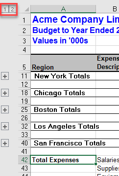
With a single click, you can expand the dataset or collapse it into just the summary rows. Click on the level number in the outline to collapse the data with only the subtotals displayed. That’s level 2 in our example outline:
 23")
All the summary rows will be in view:
 24")
Click on the last level of the outline to expand the dataset back to the detail rows (i.e. level 3 for us).
You can use these level buttons to expand or collapse the groups. For specific groups, you can make use of the Hide Detail button. Let us show you how. Let’s say we want all other than the upper 3 groups collapsed. Select the remaining dataset and click on the Hide Detail button in the Outline group of the Data tab.
 25")
The selected area of the dataset will be collapsed with its rows:
 26")
You can use the Show Detail button anytime to expand some or all of the collapsed groups again.
If you’ve practiced the methods, you should be an expert row grouper by now. We’ll tag you with a row grouping badge. You’ve earned it! And with every lesson, you get closer to being Excel experts. We’ll be back with more time-saving, troubleshooting, and Excel tooting. We’ll sign off with the hope that your badge collection is growing.
![]()
Download Article
Layer your data to stay organized
![]()
Download Article
- Preparing Your Data
- Outlining Automatically
- Outlining Manually
- Minimizing & Clearing
- Q&A
- Tips
- Warnings
|
|
|
|
|
|
Outlining (grouping) data in Excel is a great way to organize and summarize data. This feature nests your information into up to eight levels. Inner levels have the detailed data for the surrounding outer level. As long as your data has column headings and no blank rows, you can automatically group and outline automatically with Excel. This wikiHow guide teaches you how to group and outline Excel data so you can work with large data sets more efficiently.
This works on Windows and Mac!
Things You Should Know
- Prepare your data by making column or row headers and getting rid of blank rows and columns.
- Outline rows or columns automatically by selecting a cell in the data and going to Data > Group > Auto Outline.
- For the manual method, click the Group button and choose “Rows” or “Columns.”
-
1
Organize the data you want to outline. Each column should have a column header in the first row. Make sure the range you’re going to outline doesn’t contain blank rows or columns.[1]
- For a general spreadsheet guide, check out how to make a spreadsheet in Excel and format it.
- If you’re looking for Excel database info, read our guide on creating a database from an Excel spreadsheet.
- Are you using the free version of Excel and considering upgrading to Microsoft 365? See our coupon site for Staples discounts.
-
2
Optionally, create a summary row. This is also called a subtotal. You have two options for this:
- Select a cell in the data range. Go to the Data tab and click Subtotal in the Outline group.
- Insert summary rows with your own formulas. For example, you could use the SUM function to subtotal information. These can go above or below the data.
- If you place your summary rows above the data, open the dialog box in the Outline group of the Data tab (it’s the right angle with an arrow). Uncheck “Summary rows below detail.”


Advertisement
-
1
Select a cell that’s in the range you’re going to outline. This can be any cell in the data.
- Your data must have column headers and no blank lines for this feature to work.
-
2
Click the Data tab. It’s on the left side of the green ribbon that’s at the top of the Excel window. Doing so will open a toolbar below the ribbon.
-
3
Click the down arrow under the Group button. You’ll find this option on the far-right side of the Data tab. A drop-down menu will appear.
-
4
Click Auto Outline. It’s in the Group drop-down menu.
- If you receive a pop-up box that says «Cannot create an outline», your data doesn’t have an outline-compatible formula in it. You may also have some blank cells in your data or missing column headers. You’ll need to manually outline the data.


Advertisement
-
1
Select your data. Click and drag your cursor from the top-left cell of the data you want to group to the bottom-right cell of the data.
-
2
Click Data if this tab isn’t open. It’s in the left side of the green ribbon at the top of Excel.
-
3
Click Group. It’s on the right side of the Data toolbar.
-
4
Select a group option. Click Rows to minimize your data vertically, or click Columns to minimize horizontally.
-
5
Click OK. It’s at the bottom of the pop-up window. Your grouped data is all set!


Advertisement
-
1
Minimize your data. Click the [-] button at the top or on the left side of the Excel spreadsheet to hide the grouped data. In most cases, doing this will only display the final line of the data.
-
2
Clear your outline if needed. Click Ungroup to the right of the Group option, then click Clear Outline… in the drop-down menu. This will ungroup and unhide any data that was minimized or grouped previously.


Advertisement
Add New Question
-
Question
How do I reverse the grouping so that the total is at the top line and the collapsed lines fall below?

Click the «Data» tab, then come to the «Outline» section, then click the small arrow on the right bottom corner to «Show the Outline Dialog Box». From the settings, unclick «Summary Rows Below Detail.»
-
Question
My data is grouped, but I cannot see the outline symbols along the left side of my spreadsheet. What can I do?
While the document is open, go to «File,» «Options,» «Advanced,» «Display options for this worksheet.» Make sure «Show outline symbols if an outline is applied» is selected. This is necessary for every sheet where there are outlines/groupings applied.
-
Question
How do I group Rows 23 through 31 and then group Rows 32 through 36? When I do it, Excel groups Rows 23 thru 36.
You need an empty row between your two groups. Otherwise Excel will automatically merge them.
See more answers
Ask a Question
200 characters left
Include your email address to get a message when this question is answered.
Submit
Advertisement
-
You cannot use this function if the sheet is shared.
Thanks for submitting a tip for review!
Advertisement
-
Don’t use grouping/outlining if you plan to protect the worksheet. If you do, other users won’t be able to expand and collapse the rows.
Advertisement
About This Article
Article SummaryX
1. Open the Excel document.
2. Click Data
3. Click Group
4. Click Auto Outline
5. Click [-] to minimize data.
Did this summary help you?
Thanks to all authors for creating a page that has been read 1,502,469 times.
Is this article up to date?
This tutorial will demonstrate how to Group Cells (Rows / Columns) in Excel & Google Sheets.
Grouping or outlining data in Excel allows us to hide or show rows or columns depending on how much detail we wish to see on the screen. Different levels can be displayed according to your needs. Excel allows up to 8 levels of grouping. To use the group function in Excel, the data really needs to be organized in your worksheet in a specific way that works with the grouping functionality.
Manually Grouping or Ungrouping Rows
1. To group a number of rows together, first, highlight the rows you wish to group.
2. In the Ribbon, select Data > Outline > Group >Group.
3. A small minus sign will be added into the outline bar on the left of the screen. Clicking on the minus sign allows us to collapse the group and the minus sign will then change to a plus sign indicating that there is hidden data within the outline.
4. We can repeat manual grouping to add more groups to the worksheet as required.
5. As well as using the plus and minus outline symbols, we can also use the 1 or 2 in the top left hand corner of the screen to expand or collapse all the groups.
6. Clicking on the 1 will collapse all the groups while clicking on 2 will expand all the groups.
Manually Grouping or Ungrouping Columns
1. To group a number of columns together, first, highlight the columns you wish to group. This can be done if you have rows already grouped or not.
2. In the Ribbon, select Data > Outline > Group >Group to group the columns together. Repeat this until you have created all the groups that you require.
3. Once we have grouped our rows and / or columns, we can add a new level but grouping once again. This will add a third level of grouping to the outline symbols in the top left hand corner of the screen.
4. Once again, we can repeat this across our worksheet, and add up to 8 levels of grouping.
Ungrouping Rows or Columns
1. Highlight the group you wish to ungroup and then, in the Ribbon, select Data > Outline > Ungroup > Ungroup.
This will only remove the one group.
2. To remove all the grouping in the worksheet, click anywhere in the data and then, in the Ribbon, select Data > Outline > Ungroup > Clear Outline.
Auto-Outline
We can use the Auto Outline function of Excel as long as our data is logically organized so that Excel recognizes the groups within the rows and columns. There must not be any blank rows in the data and the data must be summed or subtotaled at each level.
1. Click anywhere in the data where you wish the outline to be created and then, in the Ribbon, select Data > Outline > Group > Auto Outline.
2. Excel will create as many grouping levels as the logical layout of the data allows.
How to Group Cells in Google Sheets
Google Sheets only allows us to manually group or ungroups rows and columns of data.
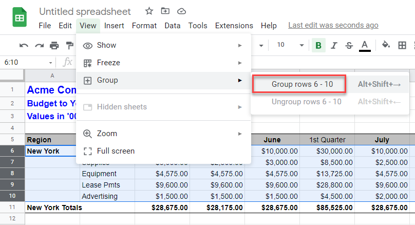
1. Select the rows you wish to group and then, in the Menu, select View > Group > Group rows (the number of rows selected will be shown).
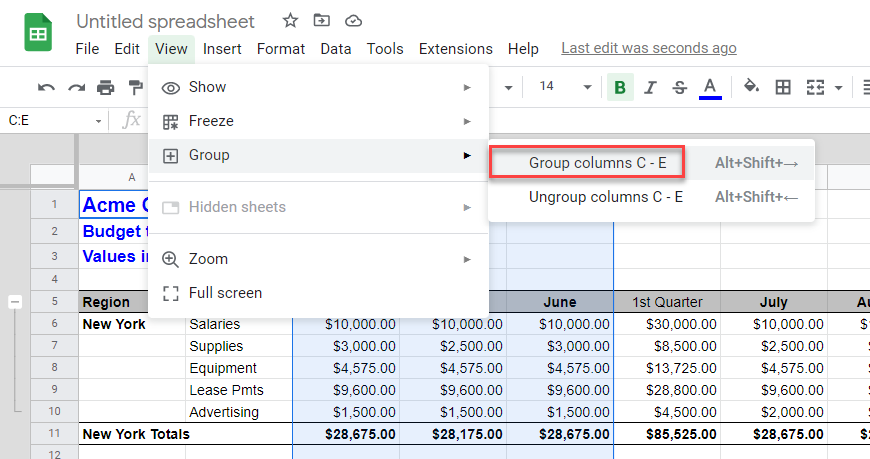
2. Similarly, select the columns you wish to group and then in the Menu, select View > Group > Group columns (the number of columns selected will be shown).
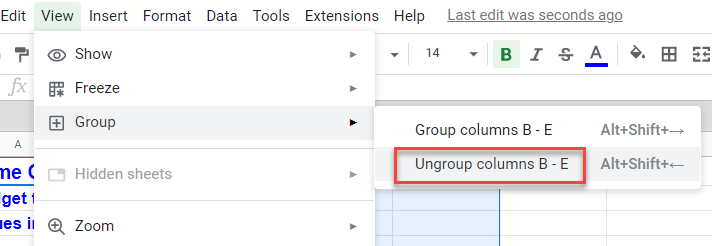
3. To ungroup rows or columns, click in the group you wish to ungroup and then in the Menu, select View > Group > Ungroup (rows or columns).
Get a handle on your data
Grouping rows and columns in Excel lets you collapse and expand sections of a worksheet. This can make large and complex datasets much easier to understand. Views become compact and organized. This article shows you step-by-step how to group and view your data.
Instructions in this article apply to Excel 2019, 2016, 2013, 2010, 2007; Excel for Microsoft 365, Excel Online and Excel for Mac.
Grouping in Excel
You can create groups by either manually selecting the rows and columns to include, or you can get Excel to automatically detect groups of data. Groups can also be nested inside other groups to create a multi-level hierarchy. Once your data is grouped, you can individually expand and collapse groups, or you can expand and collapse all groups at a given level in the hierarchy.
Groups provide a really useful way to navigate and view large and complex spreadsheets. They make it much easier to focus on the data that’s important. If you need to make sense of complex data you should definitely be using Groups and could also benefit from Power Pivot For Excel.
How to Use Excel to Group Rows Manually
To make Excel group rows, the simplest method is to first select the rows you want to include, then make them into a group.
-
For the group of rows you want to group, select the first row number and drag down to the last row number to select all the rows in the group.
-
Select the Data tab > Group > Group Rows, or simply select Group, depending on which version of Excel you’re using.
-
A thin line will appear to the left of the row numbers, indicating the extent of the grouped rows.
Select the minus (-) to collapse the group. Small boxes containing the numbers one and two also appear at the top of this region, indicating the worksheet now has two levels in its hierarchy: the groups and the individual rows within the groups.
-
The rows have been grouped and can now be collapsed and expanded as required. This makes it much easier to focus on just the relevant data.
How to Manually Group Columns in Excel
To make Excel group columns, the steps are almost the same as doing so for rows.
-
For the group of columns you want to group, select the first column letter and drag right to the last column letter, thereby selecting all the columns in the group.
-
Select the Data tab > Group > Group Columns, or select Group, depending on which version of Excel you’re using.
-
A thin line will appear above the column letters. This line indicates the extent of the grouped columns.
Select the minus (-) to collapse the group. Small boxes containing the numbers one and two also appear at the top of this region, indicating the worksheet now has two levels in its hierarchy for columns, as well as for rows.
-
The rows have been grouped and can now be collapsed and expanded as required.
How to Make Excel Group Columns and Rows Automatically
While you could repeat the above steps to create each group in your document, Excel can automatically detect groups of data and do it for you. Excel creates groups where formulas reference a continuous range of cells. If your worksheet doesn’t contain any formulas, Excel won’t be able to automatically create groups.
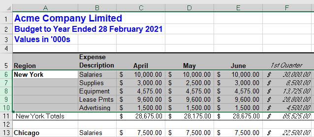
Select the Data tab > Group > Auto Outline and Excel will create the groups for you. In this example, Excel correctly identified each of the groups of rows. Because there’s no annual total for each spending category, it has not automatically grouped the columns.
This option isn’t available in Excel Online, if you’re using Excel Online, you’ll need to create groups manually.
How to Create a Multi-Level Group Hierarchy in Excel
In the previous example, categories of income and expense were grouped together. It would make sense to also group all of the data for each year. You can do this manually by applying the same steps as you used to create the first level of groups.
-
Select all of the rows to be included.
-
Select the Data tab > Group > Group Rows, or select Group, depending on which version of Excel you are using.
-
Another thin line will appear to the left of the lines representing the existing groups and indicating the extent of the new group of rows. The new group encompasses two of the existing groups and there are now three small numbered boxes at the top of this region, signifying the worksheet now has three levels in its hierarchy.
-
The spreadsheet now contains two levels of groups, with individual rows within the groups.
How to Automatically Create Multi-Level Hierarchy
Excel uses formulas to detect multi-level groups, just as it uses them to detect individual groups. If a formula references more than one of the other formulas which define groups, this indicates these groups are part of a parent group.
Keeping with the cash flow example, if we add a Gross Profit row to each year, which is simply the income minus the expenses, then this allows Excel to detect that each year is a group and the income and expenses are sub-groups within these. Select the Data tab > Group > Auto Outline to automatically create these multi-level groups.
How to Expand and Collapse Groups
The purpose of creating these groups of rows and/or columns is that it allows regions of the spreadsheet to be hidden, providing a clear overview of the entire spreadsheet.
-
To collapse all of the rows, select the number 1 box at the top of the region to the left of the row numbers.
-
Select the number two box to expand the first level of groups and make the second level of groups visible. The individual rows within the second level groups remain hidden.
-
Select the number three box to expand the second level of groups so the individual rows within these groups also become visible.
It’s also possible to expand and collapse individual groups. To do so, select the Plus (+) or Minus (-) that appears to mark a group that’s either collapsed or expanded. In this way, groups at different levels in the hierarchy can be viewed as required.
Thanks for letting us know!
Get the Latest Tech News Delivered Every Day
Subscribe