
Return to Charts Home
This tutorial will demonstrate how to graph a Function in Excel & Google Sheets.
How to Graph an Equation / Function in Excel
Set up your Table
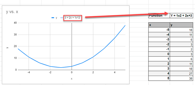
- Create the Function that you want to graph
- Under the X Column, create a range. In this example, we’re range from -5 to 5
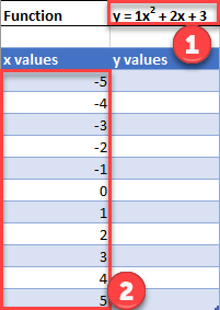
Fill in Y Column
Create a formula using the Function, substituting x with what is in Column B.
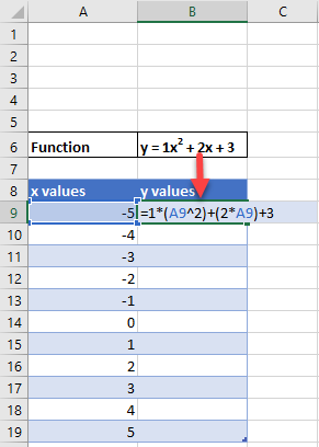
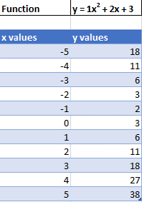
After using this formula for all the rows, you should have a table that looks like below.
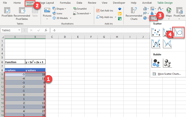
Creating Scatterplot
- Highlight Dataset
- Select Insert
- Select Scatterplot
- Select Scatter with Smooth Lines
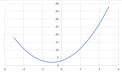
This will create a graph that should look similar to below.
Add Equation Formula to Graph
- Click Graph
- Select Chart Design
- Click Add Chart Element
- Click Trendline
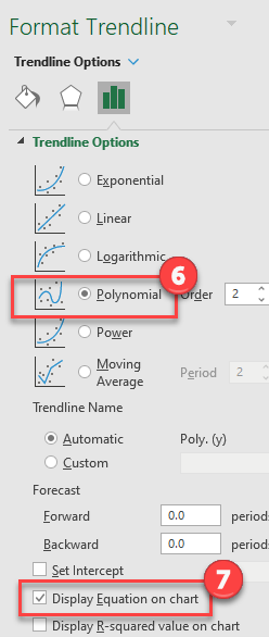
- Select More Trendline Options
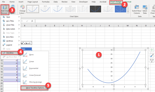
6. Select Polynomial
7. Check Display Equation on Chart
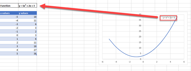
Final Scatterplot with Equation
Your final equation on the graph should match the function that you began with.
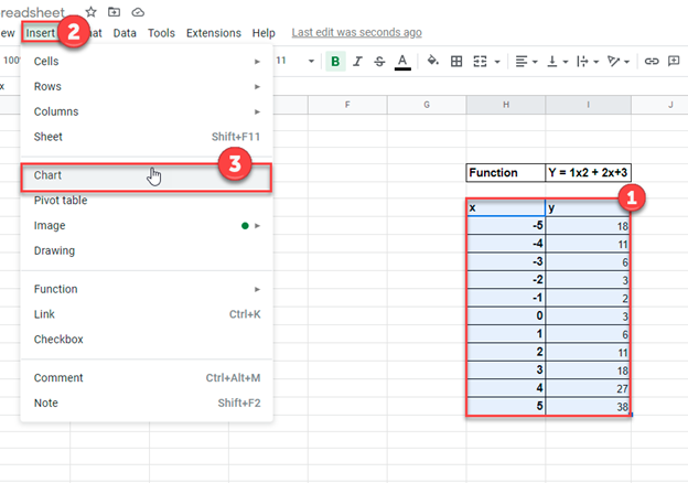
How to Graph an Equation / Function in Google Sheets
Creating a Scatterplot
- Using the same table that we made as explained above, highlight the table
- Click Insert
- Select Chart
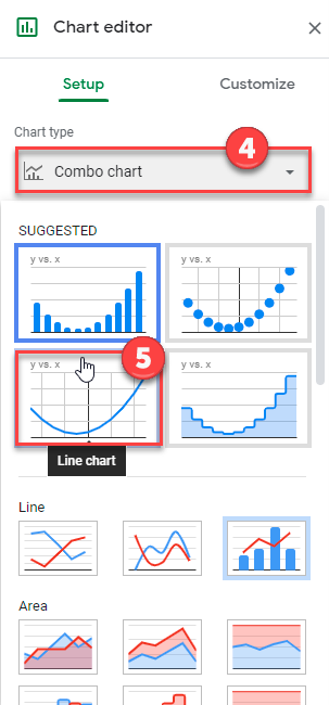
4. Click on the dropdown under Chart Type
5. Select Line Chart
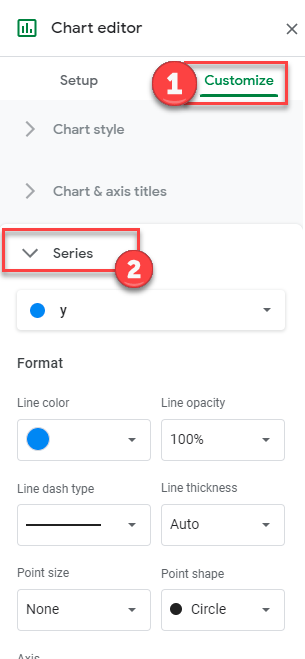
Adding Equation
- Click on Customize
- Select Series
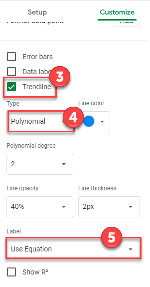
3. Check Trendline
4. Under Type, Select Polynomial
5. Under Label, Select Use Equation
Final Scatterplot with Equation
As you can see, similar to the exercise in Excel, the equation matches the function that we began with.
Often you may be interested in plotting an equation or a function in Excel. Fortunately this is easy to do with built-in Excel formulas.
This tutorial provides several examples of how to plot equations/functions in Excel.
Example 1: Plot a Linear Equation
Suppose you’d like to plot the following equation:
y = 2x + 5
The following image shows how to create the y-values for this linear equation in Excel, using the range of 1 to 10 for the x-values:

Next, highlight the values in the range A2:B11. Then click on the Insert tab. Within the Charts group, click on the plot option called Scatter.

The following plot will automatically appear:

We can see that the plot follows a straight line since the equation that we used was linear in nature.
Example 2: Plot a Quadratic Equation
Suppose you’d like to plot the following equation:
y = 3x2
The following image shows how to create the y-values for this equation in Excel, using the range of 1 to 10 for the x-values:

Next, highlight the values in the range A2:B11. Then click on the Insert tab. Within the Charts group, click on the plot option called Scatter.
The following plot will automatically appear:

We can see that the plot follows a curved line since the equation that we used was quadratic.
Example 3: Plot a Reciprocal Equation
Suppose you’d like to plot the following equation:
y = 1/x
The following image shows how to create the y-values for this equation in Excel, using the range of 1 to 10 for the x-values:

Next, highlight the values in the range A2:B11. Then click on the Insert tab. Within the Charts group, click on the plot option called Scatter.
The following plot will automatically appear:

We can see that the plot follows a curved line downwards since this represents the equation y = 1/x.
Example 4: Plot a Sine Equation
Suppose you’d like to plot the following equation:
y = sin(x)
The following image shows how to create the y-values for this equation in Excel, using the range of 1 to 10 for the x-values:

Next, highlight the values in the range A2:B11. Then click on the Insert tab. Within the Charts group, click on the plot option called Scatter with Smooth Lines and Markers.
The following plot will automatically appear:

Conclusion
You can use a similar technique to plot any function or equation in Excel. Simply choose a range of x-values to use in one column, then use an equation in a separate column to define the y-values based on the x-values.
Contents
- 1 How do you plot an equation?
- 2 Can I plot a function in Excel?
- 3 How do I graph an equation in Excel 2016?
- 4 Is an equation a formula?
- 5 How do you find the equation of a line?
- 6 What is graph of quadratic equation?
- 7 What is Y MX B?
- 8 What are formulas in Excel?
- 9 What is an example of a equation?
- 10 How do you find the equation of a line that has the given slope and passes through the given point?
- 11 Can Excel solve a quadratic equation?
- 12 Can Excel solve equations?
- 13 How do you solve for a variable in an equation in Excel?
To graph an equation using the slope and y-intercept, 1) Write the equation in the form y = mx + b to find the slope m and the y-intercept (0, b). 2) Next, plot the y-intercept. 3) From the y-intercept, move up or down and left or right, depending on whether the slope is positive or negative.
Can I plot a function in Excel?
A quick and easy way to plot y = f(x) functions in Excel available with the XLSTAT add-on statistical software. This tool allows you to plot a function of the type y = f (x) on an existing or new chart.
How do I graph an equation in Excel 2016?
On the Layout tab, in the Analysis group, click Trendline, and then click More Trendline Options. To display the trendline equation on the chart, select the Display Equation on chart check box.
Is an equation a formula?
An equation is any expression with an equals sign, so your example is by definition an equation. Equations appear frequently in mathematics because mathematicians love to use equal signs. A formula is a set of instructions for creating a desired result.
How do you find the equation of a line?
To find an equation of a line given the slope and a point.
- Identify the slope.
- Identify the point.
- Substitute the values into the point-slope form, y − y 1 = m ( x − x 1 ) .
- Write the equation in slope-intercept form.
What is graph of quadratic equation?
The graph of a quadratic function is a U-shaped curve called a parabola.The extreme point ( maximum or minimum ) of a parabola is called the vertex, and the axis of symmetry is a vertical line that passes through the vertex. The x-intercepts are the points at which the parabola crosses the x-axis.
What is Y MX B?
y = mx + b is the slope intercept form of writing the equation of a straight line. In the equation ‘y = mx + b’, ‘b’ is the point, where the line intersects the ‘y axis’ and ‘m’ denotes the slope of the line. The slope or gradient of a line describes how steep a line is.
What are formulas in Excel?
A formula is an equation that makes calculations based on the data in your spreadsheet. Formulas are entered into a cell in your worksheet. They must begin with an equal sign, followed by the addresses of the cells that will be calculated upon, with an appropriate operand placed in between.
What is an example of a equation?
An equation is a mathematical sentence that has two equal sides separated by an equal sign. 4 + 6 = 10 is an example of an equation. We can see on the left side of the equal sign, 4 + 6, and on the right hand side of the equal sign, 10.For example, 12 is the coefficient in the equation 12n = 24.
How do you find the equation of a line that has the given slope and passes through the given point?
These are the two methods to finding the equation of a line when given a point and the slope:
- Substitution method = plug in the slope and the (x, y) point values into y = mx + b, then solve for b.
- Point-slope form = y − y 1 = m ( x − x 1 ) , where ( x 1 , y 1 ) is the point given and m is the slope given.
Can Excel solve a quadratic equation?
A quadratic equation can be solved by using the quadratic formula. You can also use Excel’s Goal Seek feature to solve a quadratic equation.We can solve the quadratic equation 3x2 – 12x + 9.5 – 24.5 = 0 by using the quadratic formula.
Can Excel solve equations?
The Solver in Excel can perform many of the same functions as EES and MathCAD. It can be used to solve single equations (for example x2+3x-22=5) or multiple equations (for example x3-14x=z, z12-1=x2+1).
How do you solve for a variable in an equation in Excel?
How to Use Solver in Excel
- Click Data > Solver. You’ll see the Solver Parameters window below.
- Set your cell objective and tell Excel your goal.
- Choose the variable cells that Excel can change.
- Set constraints on multiple or individual variables.
- Once all of this information is in place, hit Solve to get your answer.
The equation having the highest degree is 1 is known as a linear equation. If we plot the graph for a linear equation, it always comes out to be a straight line. There are different forms of linear equations such as linear equations in one variable, and linear equations in two variables.
- Linear equations in one variable: standard form of this equation is ‘ax + b = 0’, where a and b are real numbers and x is a variable.
- Linear equation in two variables: standard form or this equation is, ‘ax + by = c’, where a, b and c are real numbers, and x is a variable.
Graph a linear equation using Excel
Graph of Linear equation (one variable)
In only one variable, the value of only one variable is needed to be found. Therefore, the equation can be solved directly. Let’s take one linear equation in one variable i.e 2x + 3 = 9.
Step 1: Solve the linear equation
2x + 3 = 9
2x = 9 – 3
2x = 6
x = 6/2
x = 3
Step 2: Plot the graph
For a linear equation in one variable, the graph will always have a line parallel to any axis.
For x = 3, the graph will be a line parallel to the y-axis which intersects the x-axis at 3, because for any value of y, the value of x is 3. Below table data can be used to plot the graph,

Co-ordinates taken is (3, 0), (3, 5), (3, 10), (3, 15), (3, -5), (3, -10), (3, -15).
Plot the graph using the following steps
Step 1: Select the data

Step 2: Click on the ‘Insert’ tab and select scatter with marker chart.

Output

Graph of Linear equation (two variables)
Let’s take one linear equation in one variable i.e 2x + 3y = 6. In order to get the data points for plotting the graph, assume some value of x and find the corresponding y value.
For example, If x = 0
Substitute value of x in given equation,
2(0) + 3y = 6
3y = 6
y = 2
Then, the data point is (0, 2). Similarly, we can get different coordinates, those are (3, 0), (-3, 4), and (6, -2).

Plot the graph using the following steps
Step 1: Select the data

Step 2: Click on the ‘Insert’ tab and select scatter with marker chart.

Output

Graphs are a common visual aid in the worlds of business, finance and industries where progress and management are a critical part of achieving success. Excel is a program that gives users the opportunity to make tables, enter data, organize information and create graphs that correspond with specific equations. If you’re interested in pursuing a profession that requires entering data and generating graphs, understanding the processes necessary for programs like Microsoft Excel can be helpful for advancing in your career.In this article, we discuss scenarios when you may want to add an equation to a graph in Excel, describe why it’s important to include supplemental information like equations, list a step-by-step guide for formatting your graph and equation on your own and provide several tips to help create your own graphs with equations using Microsoft Excel.
Why is it important to add an equation to a graph in Excel?
Its important to add an equation next to your trendline on a graph because it gives your audience ample information regarding your calculations. If they wanted to, they could take your equation from the worksheet and plug in their own values to determine how it would affect the trajectory of the graph and, therefore, how different values affect the trendline and the factors it represents. For example, if you were presenting your data and graph to a group of investors for a clothing company, you may include the equation to give them the ability to plug in future values and make predictions about future sales or production.
When to add an equation to a graph in Excel
There are some common instances where including an equation can be beneficial on a graph using Excel. Here are some of the most common instances when you may want to add an equation to your Excel graph:
Forecasting trends
For people in fields like business, finance or technology, a common method of predicting performance is by turning data sets into graphs. The addition of a trendline to a graph gives the audience an idea of the trajectory of the values, which they can use to make business decisions, such as ordering stock, introduction of new products or marketing campaigns and even what times of year are most profitable. If presenting your graph to a team of investors or strategists, they can use the equation displayed on the chart to make their own forecasts using calculations.
Scholarly work
Another common reason individuals add equations to their graphs is if theyre working on a scholarly article or other academic work. In academia, many people add equations next to their graphs to provide the reader of the work with as much information as possible. It gives your audience the ability to test out their calculations and can be a pivotal part of the peer-review process. Its also common for many high school and undergraduate courses to require students to include their equations as part of their graphs, as it demonstrates to the instructor whether theyve made the right calculations for their data.
How to add an equation to a graph in Excel
Here are the steps you can follow to add an equation to a graph in Microsoft Excel:
1. Enter data into Excel
The first step in the process of adding an equation to your graph in Excel is to open the application on your computer or by accessing it through your web browser. Once on the homepage, navigate to the worksheet and begin entering your data to create a table. For a typical linear graph, you can create two columns with titles and their corresponding values listed beneath. This is the data that you will transform into your graph, where you will eventually add your equation.
2. Transform your table into a graph
The next step is to transform your dataset into a graph using Excel. To do this, highlight the table you created on the worksheet and scroll to the top bar of the screen. Click the “Insert” tab, which should open up a variety of features to add to your worksheet, and navigate to the middle where you can choose from different graph formats. Select the one that resembles a scatter chart and click the same icon once again when the drop down opens to turn the data in your table into a graph with points representing your values.
3. Open “Format Trendline” side pane
Once your graph appears on your worksheet, the next step is to add your trend line. To do this, start by clicking anywhere on your graph to reveal the “+” icon next to your chart, and click that to open up a drop down where you can make add or remove axes, titles, labels, grid lines, the legend and your trendline. Hover over “Trendline” to reveal an arrow which should open up another drop down. Click “More Options…” to open the “Format Trendline” side pane.
4. Click “Display Equation on Chart”
After opening the “Format Trendline” side pane, you can make selection regarding the style of your graph. Click the icon with the three bars to open the “Trendline Options” drop down, where you can select the type of trendline you want on your graph, such as linear or exponential. Navigate downwards on the pane where you have the option to check mark three boxes. Check the box next to “Display Equation on chart” to ensure that the equation appears on your final graph.
5. Save and share your graph
Once youve checked the “Display Equation on chart” box, the equation that corresponds with your data should appear adjacent to your trendline on your graph. After checking that your values and graph correctly coincide with each other, you can save your worksheet by navigating to the top bar of your screen. Click “File” and “Save as” to name your Excel worksheet and save it to your files. If you want to share your worksheet, navigate to the top right corner of the screen and click “Share” to invite others, copy the link or send a copy of your work.
Tips for adding equations to a graph in Excel
Here are some tips you can use as a reference when adding equations to your Excel graphs:
Please note that none of the companies mentioned in this article are affiliated with Indeed.
Want to graph trigonometric equations, but don’t know where to start? Here’s how to do it in Excel like a pro.

Visualizing trigonometric equations is an important step in understanding the relationship between the X and Y axis. Without a graph, guessing a complex trigonometric equation’s behavior can become quite a challenge. Fortunately, Microsoft Excel is an excellent tool for graphing and visualizing data, including trigonometric equations.
Visualizing an equation makes it easier to grasp, and once you’ve got the hang of graphing trigonometric equations with Excel, you’ll have a better time understanding trigonometry. In this article, we’ll explain how to use Excel to graph trigonometric equations and provide a step-by-step example to help you get started.
How to Graph Trigonometric Equations With Excel
To graph an equation with Excel, you’ll need to create a chart for the X and Y values. The good news is that you don’t have to manually calculate the Y values, as Excel has an arsenal of trigonometric functions built into it.
All you need to do is create a data table with the X values, and then write an Excel formula to automatically calculate the Y values. With your data table ready, you can create an Excel chart to graph the equation.
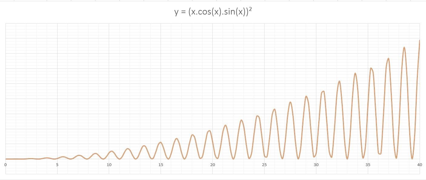
Now let’s put this outline to use and graph the y = (x.cos(x).sin(x))² equation. This equation is tough to imagine just by looking at it, but you can save yourself the burden by quickly graphing the equation with Excel.
1. Input the X Values
A graph needs X and Y values. You can enter the domain you want to graph in the X values, and then calculate the Y values with a formula in the next step. It’s a good idea to create a table for your data, as it will enable Excel’s autofill feature.
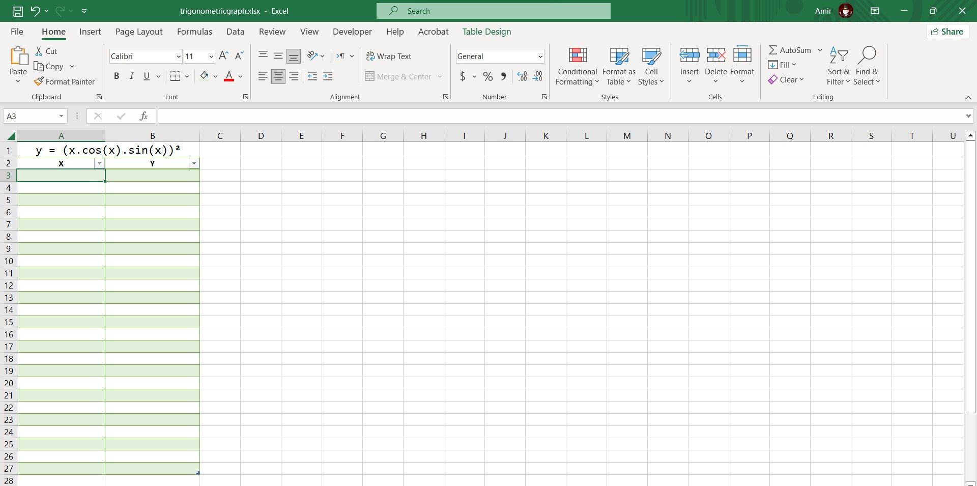
The smaller the increment between your X values is, the more accurate your graph will be. We’re going to have each X value increase by 1/4 in this table. Here’s how you can automatically input the X values:
- Type in the first value in a cell. In this example, we’re going to type -3 in cell A3.
- Select the cell below. That’s A4 in our case.
- In the formula bar, enter the formula below:
=A3+1/4 - Press Enter.
- Grab the fill handle and drop it into the cells below.
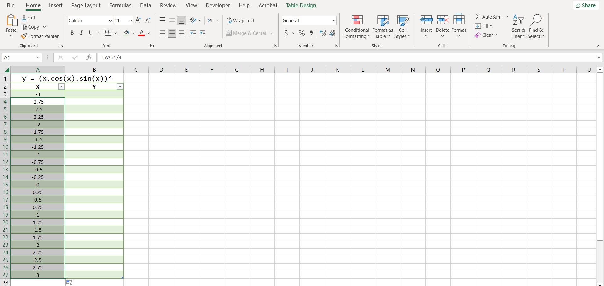
Excel will now fill in all the other X values. The advantage of using a formula to input the values is that you can now quickly change the values by editing the first value or altering the formula.
2. Create a Formula to Calculate the Y Values
With the X values in place, it’s time to calculate the Y values. You can calculate the Y values by translating the trigonometric equation into Excel’s language. It’s essential that you have an understanding of the trigonometric functions in Excel to proceed with this step.
When creating your formula, you can use a circumflex (^) to specify the power. Use parentheses where needed to indicate the order of operations.
- Select the first cell where you want to calculate the Y value. That’s B3 in our case.
- Go to the formula bar and enter the formula below:
=(A3*COS(A3)*SIN(A3))^2 - Press Enter.
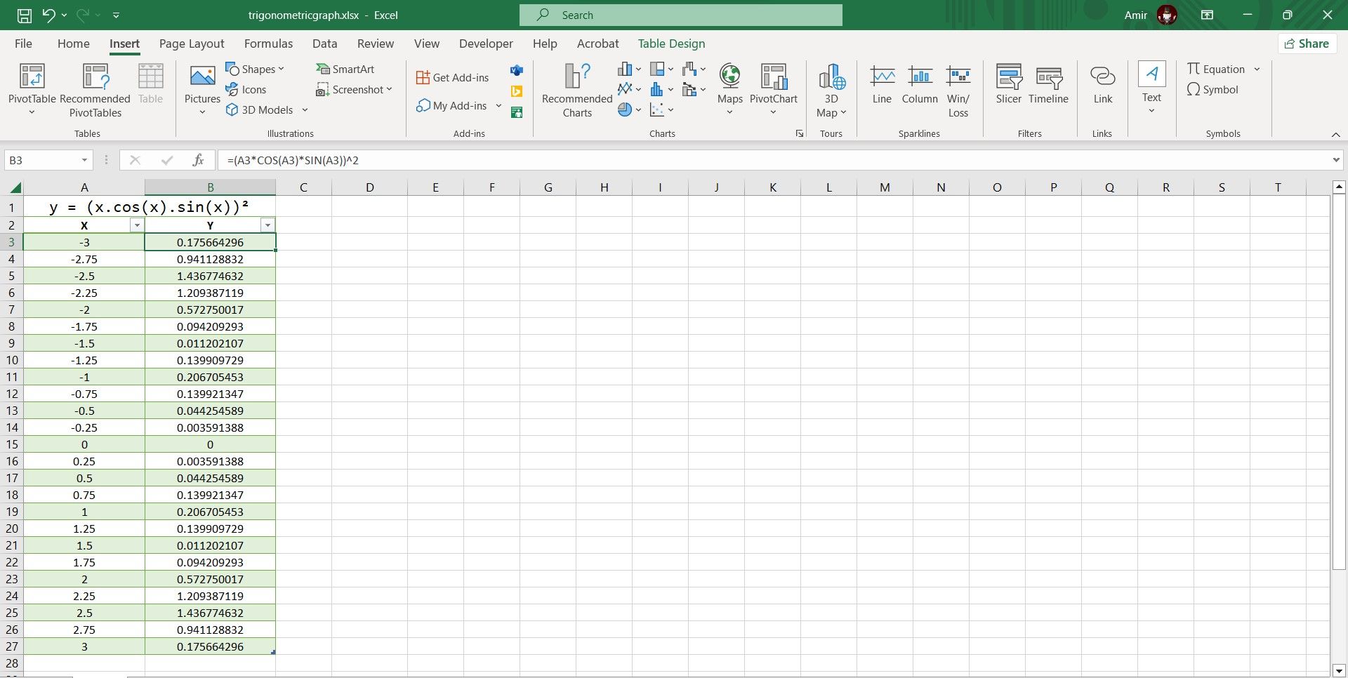
Excel will now calculate all Y values in the table. Excel’s trigonometric functions use radians, so this formula will perceive the X values as radians as well. If you want your X-axis to be on a pi-radian scale rather than a radian scale, you can multiply the cell reference by pi using the PI function in Excel.
=(A3*PI()*COS(A3*PI())*SIN(A3*PI()))^2
The formula above will output the Y values for the same trigonometric equation, but the values will be on a pi-radian scale instead.
3. Create a Scatter Plot Chart
A scatter plot is the best way to graph a trigonometric equation in Excel. Since you’ve got your X and Y values ready, you can graph your equation with a single click:
- Select the table containing the X and Y values.
- Go to the Insert tab.
- In the Charts section, click on Scatter and then select Scatter with Smooth Lines.
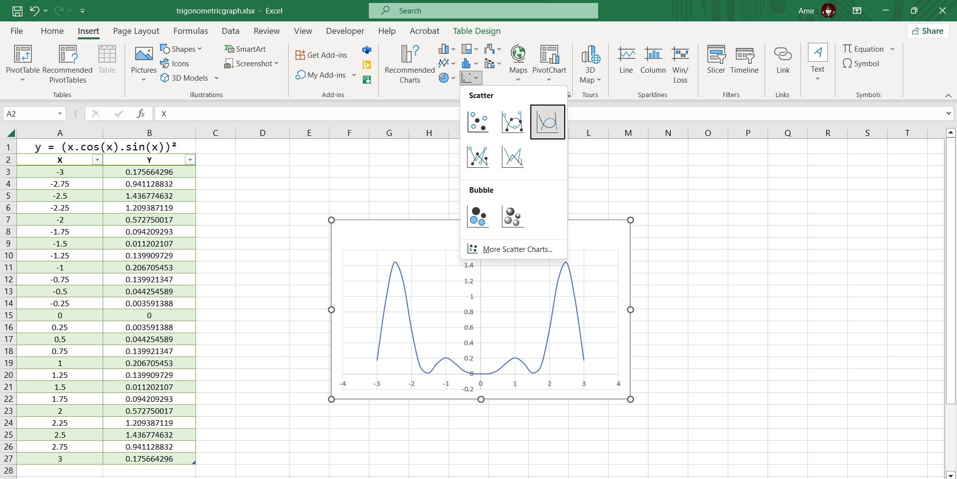
There you have it! You can now inspect the graph to better understand the equation’s behavior. This is the last step if you’re looking for a quick visualization, but if you want to present the graph, you can fully customize the Excel chart to properly graph the trigonometric equation.
4. Modify the Excel Chart
Although the chart does display the graph, you can make some changes to improve the chart’s readability and make it more presentable. There are lots of things you can customize to improve the chart, and in the end, it’s a matter of personal preference. Still, here are some adjustments that can always improve your trigonometric graph.
I. Set the Axis Units and Add Tick Marks
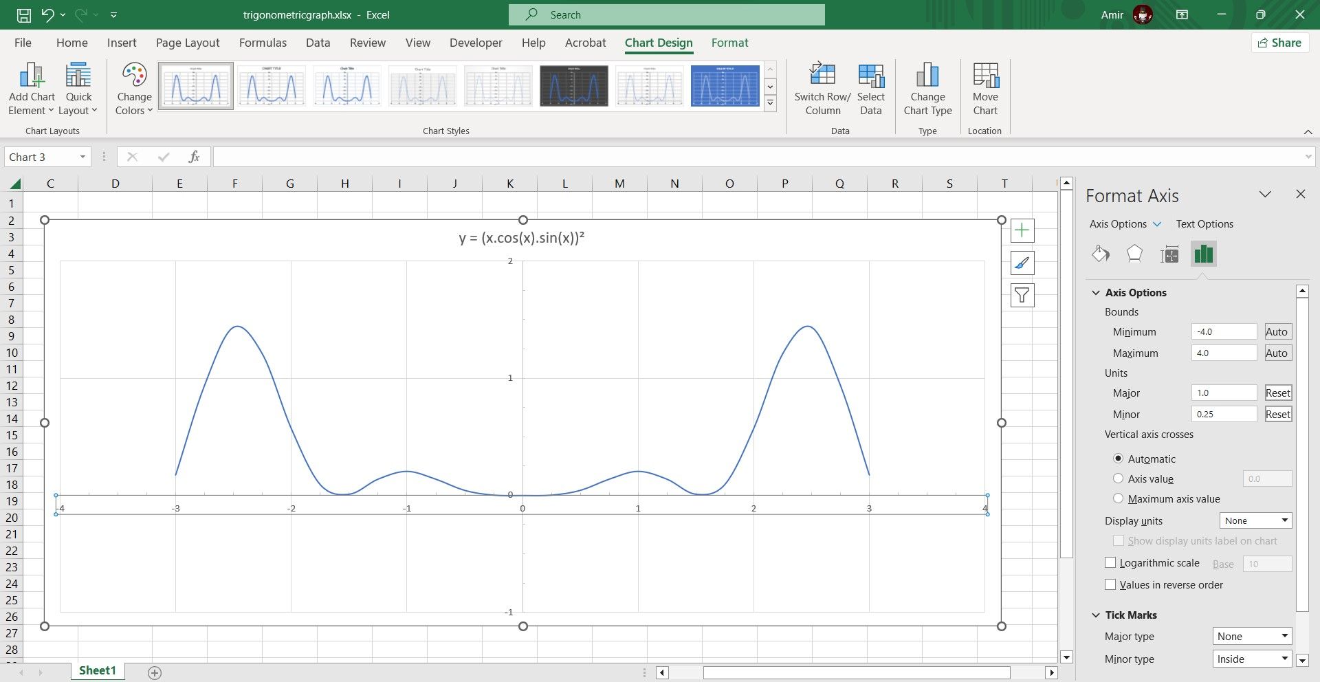
If you take a closer look at your chart, you’ll see that the horizontal and vertical grid lines aren’t the same unit. Here’s how you can fix that:
- Click on the chart to select it.
- Double-click the axis. This will bring up Format Axis on the right.
- In Format Axis, find Units under Axis Options and change Major and Minor.
- Go to Tick Marks and change Minor type to what you want.
Repeat the same process for the other axis, and make sure that you use the same major and minor units for both. Your graph should look tidier now.
II. Add Minor Gridlines
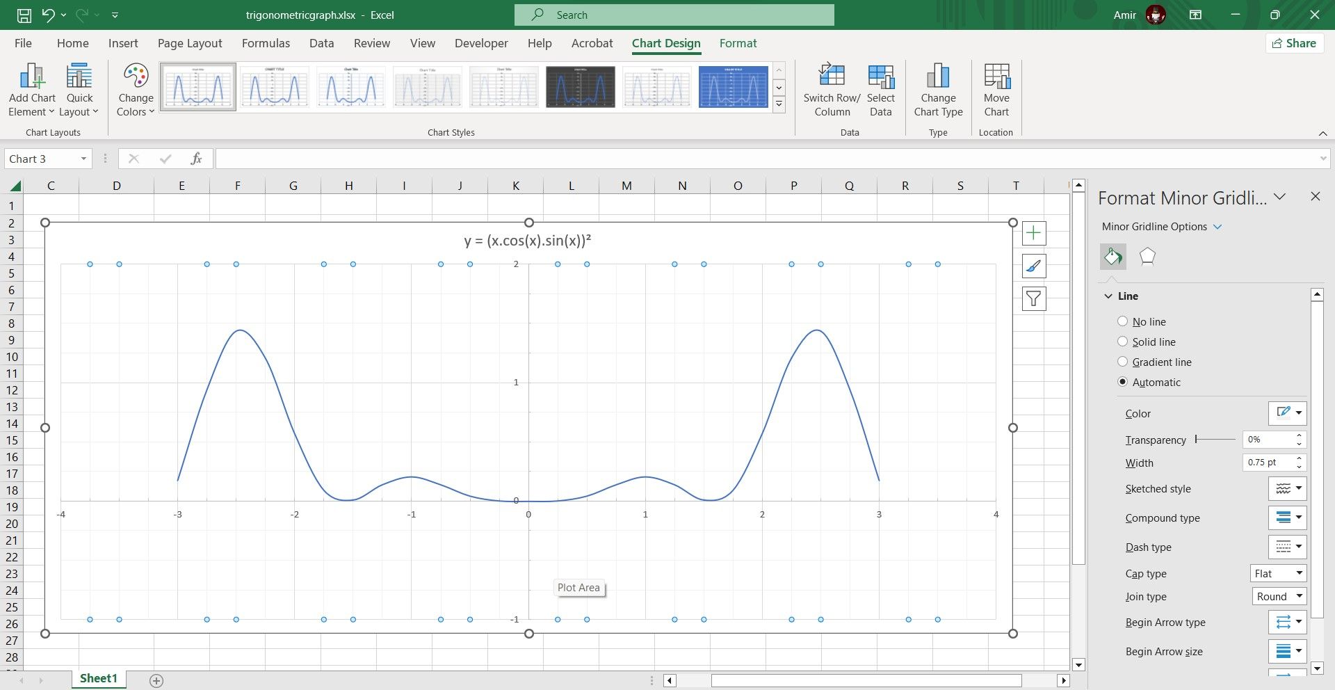
You can add minor gridlines to make the graph easier to read. To do this, simply right-click on the axis and then select Add Minor Gridlines. Repeat the process for the other axis to add gridlines there as well. You can then right-click the axis and select Format Minor Gridlines to change their appearance.
III. Add Axis Titles
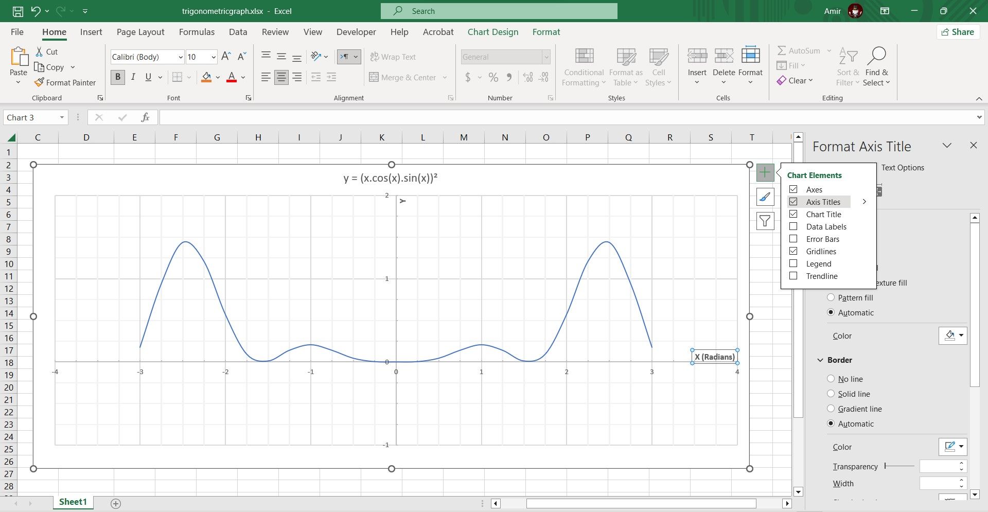
Although it’s obvious that the horizontal axis is displaying the X values, you can add a title to specify that the values are in radians. This prevents confusion with pi-radians.
- Select the chart.
- Click on Chart Elements on the top right. This is marked with a + sign.
- Select Axis Titles.
- Double-click the axis titles and edit the text.
IV. Add Data Callouts
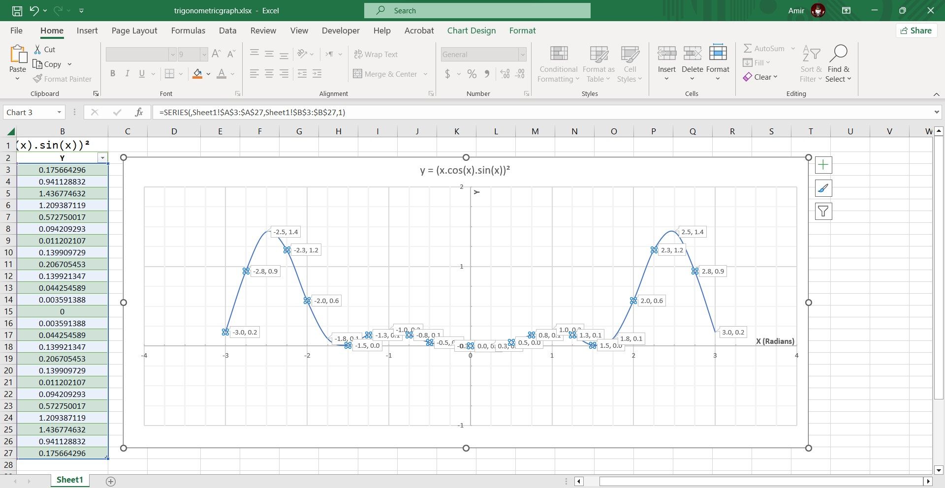
Finally, you can add callouts to identify the minimum and maximum points on your graph. Here’s how you can do that:
- Select the chart.
- Right-click the series line.
- Go to Add Data Labels and then select Add Data Callouts.
If some of the callouts seem unnecessary to you, you can individually select them and then press Del on your keyboard to delete the callout.
Graph It Properly With Excel
Visualizing an equation is vital to understanding it. This is especially true when you’re dealing with complex trigonometric equations and can’t quickly guess the values. Well, there’s no need to tax your brain to get a mental image of an equation. You can use Excel to efficiently graph a trigonometric function.
The only elements that you need to manually input are the starting X value and the increment. From there, you can have Excel automatically fill in the X values. Thanks to its array of trigonometric functions, you can easily turn your equation into an Excel formula and calculate the Y values as well.
With both the X and Y values set out in a table, graphing the equation is only a matter of selecting the data and creating a scatter plot to visualize it.
Graph a Functions or an Equation in Excel
A common question new Excel users ask is «How can I graph an
equation?» Excel allows you to draw nice curves of all the formulas you wish. If you are a student or scientist and in
order to visualize a process described by an equation, plotting the equation
is the easiest. You can see our tutorial in our graph a
function page.
In this page we show you an example template that will let you graph any functions in Excel.
Then you can move it along the axes, zoom in and zoom out of the function
You can trace any function you like, linear Function, Exponentials, Trigonometric formulas.
Plot any of these
functions by selecting them among the ones given in the example. A picture
is worth 1000 words. Same for curves and graphs. Try this spreadsheet.
The spreadsheet graph template will let you draw curves as
follow. There is a version with Macro and one without macro. You might not
like macro because of safety reasons but the macro version allows you to use
button to change the scales.
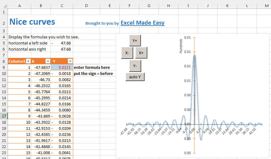
You can enter any function in a very easy way. Just enter it
in the blue cell in the x form. Like here in these examples:
- sin(x)/x
- sin(x)/abs(x)
- x*sin(1/x)
- sin(x-1)/(x-1)
- (1-sin(x))/(cos(x)*cos(x))
- x/abs(x)
- log(x)/x
- x^2+4*x-5
- x^3-4*x^2-24*x-12
You can create your owns of course.
You can download the spreadsheet template version is
here. The Macro allows
you to zoom in and zoom out of the function.