
Find and remove duplicates
Excel for Microsoft 365 Excel 2021 Excel 2019 Excel 2016 Excel 2013 Excel 2010 Excel 2007 Excel Starter 2010 More…Less
Sometimes duplicate data is useful, sometimes it just makes it harder to understand your data. Use conditional formatting to find and highlight duplicate data. That way you can review the duplicates and decide if you want to remove them.
-
Select the cells you want to check for duplicates.
Note: Excel can’t highlight duplicates in the Values area of a PivotTable report.
-
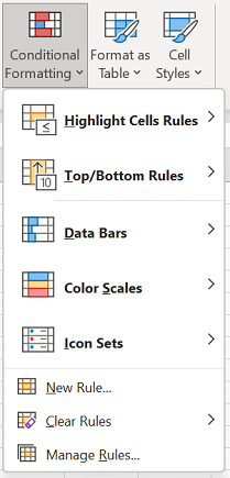
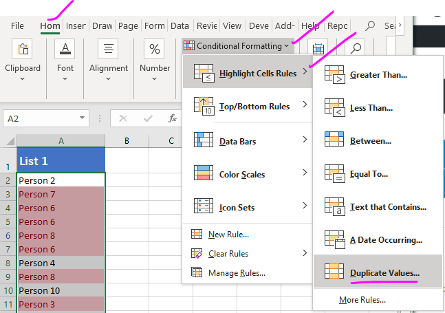
Click Home > Conditional Formatting > Highlight Cells Rules > Duplicate Values.

-
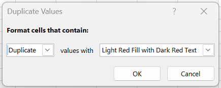
In the box next to values with, pick the formatting you want to apply to the duplicate values, and then click OK.
Remove duplicate values
When you use the Remove Duplicates feature, the duplicate data will be permanently deleted. Before you delete the duplicates, it’s a good idea to copy the original data to another worksheet so you don’t accidentally lose any information.
-
Select the range of cells that has duplicate values you want to remove.
-
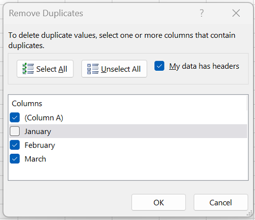
Click Data > Remove Duplicates, and then Under Columns, check or uncheck the columns where you want to remove the duplicates.
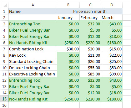
For example, in this worksheet, the January column has price information I want to keep.
So, I unchecked January in the Remove Duplicates box.
-
Click OK.
Note: The counts of duplicate and unique values given after removal may include empty cells, spaces, etc.
Need more help?

Need more help?
In MS Excel, the duplicate values can be found and removed from a data set. Depending on your data and requirement, the most commonly used methods are the conditional formatting feature or the COUNTIF formula to find and highlight the duplicates for a specific number of occurences. The columns of the data set can be then filtered to view the duplicate values.
In this article, we will look at 5 different methods to check, identify, and delete duplicates in Excel.
Table of contents
- How to Find Duplicates in Excel?
- 5 Methods to Check & Identify Duplicates in Excel
- #1 – Conditional Formatting
- #2 – Conditional Formatting (Specific Occurrence)
- #3 – Change Rules (Formulas)
- #4 – Remove Duplicates
- #5 – COUNTIF Formula
- Frequently Asked Questions
- Recommended Articles
- 5 Methods to Check & Identify Duplicates in Excel
5 Methods to Check & Identify Duplicates in Excel
You can download this Find for Duplicates Excel Template here – Find for Duplicates Excel Template
#1 – Conditional Formatting
The conditional formattingConditional formatting is a technique in Excel that allows us to format cells in a worksheet based on certain conditions. It can be found in the styles section of the Home tab.read more feature is available in Excel 2007 and subsequent versions.
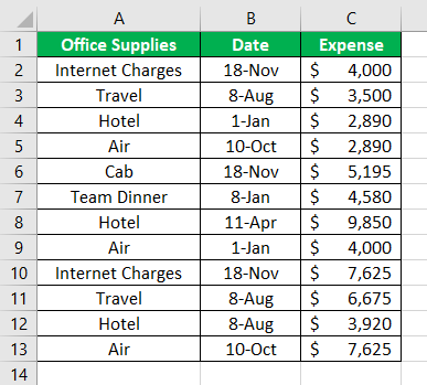
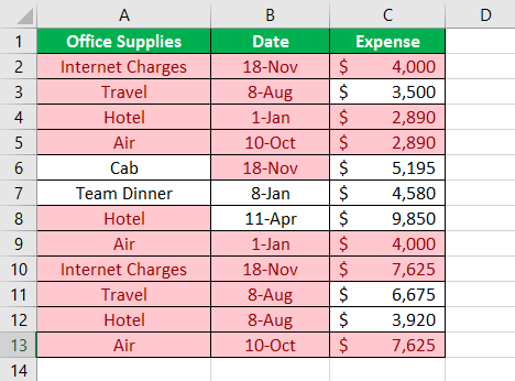
The following table consists of the expenses incurred on availing certain office facilities. The corresponding dates of purchasing such facility are also listed.
We want to identify the duplicates in excel with the help of conditional formatting.
The steps to find the duplicates in excel with the help of conditional formatting are listed as follows:
- Select the data range (A1:C13) where duplicates are to be found.
- In the Home tab, select “conditional formatting” from the “styles” section. From the drop-down menu, select “highlight cell rules” and click on “duplicate values.”

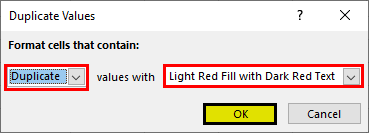
- The pop-up window titled “duplicate values” appears. In the first box on the left side, select “duplicate.” In the “values with” drop-down, select the required color to highlight the duplicate cells. Click “Ok.”

- The duplicate cells are highlighted in the data table, as shown in the following image.

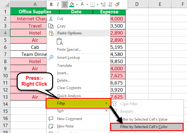
- The columns can be filtered to identify the duplicate values. For this, right-click the required column and select “filter by selected cell’s color.” The data is filtered for duplicates.

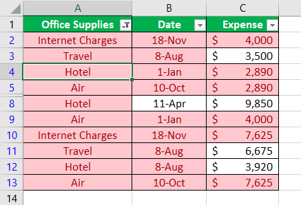
- The result after applying the filter to the first column (office supplies) is shown in the following image.

#2 – Conditional Formatting (Specific Occurrence)
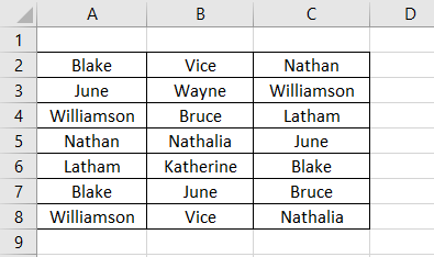
Let us consider an example to identify the specific number of duplications. In the following table, we want to check and show the duplicate values with three occurrences.
The steps to find the duplicate values for specific number of occurrences are listed as follows:
Step 1: Select the range A2:C8 in the given data table.
Step 2: In the Home tab, select “conditional formatting” from the “styles” section. Click “new rule.”
Note: The “new rule” option helps highlight a specific count of duplicates using the COUNTIF formula.
Step 3: The pop-up window titled “new formatting rule” appears. Enter the following details, as shown in the succeeding image.
- Under “select a rule type,” select “use a formula to determine which cells to format.”
- Under “edit the rule description,” enter the COUNTIFThe COUNTIF function in Excel counts the number of cells within a range based on pre-defined criteria. It is used to count cells that include dates, numbers, or text. For example, COUNTIF(A1:A10,”Trump”) will count the number of cells within the range A1:A10 that contain the text “Trump”
read more formula.
The COUNTIF formula “=COUNTIF(cell range of the data table, cell criteria)” finds and highlights the cells for the desired number of occurrences.
In this case, the COUNTIF formula highlights duplicate cells having triplicate count. This count can be changed to a greater number. The conditions can also be changed depending on the user’s requirement.
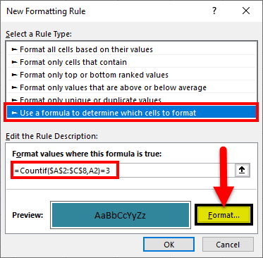
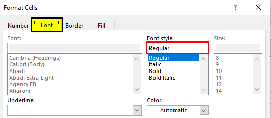
Step 4: Once the COUNTIF formula is entered, click “format.” The pop-up window titled “format cells” opens. Select the font style “regular.”
Step 5: In the “fill” tab, select blue color. The “fill” tab helps highlight the duplicate cellsHighlight Cells Rule, which is available under Conditional Formatting under the Home menu tab, can be used to highlight duplicate values in the selected dataset, whether it is a column or row of a table.read more.
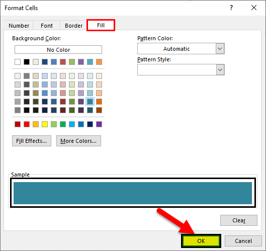
Step 6: Once the selections in “format cells” window are complete, click “Ok.” Click “Ok” again in the “new formatting rule” window.
Step 7: The result is displayed in the following image. The duplicate cells with three occurrences are highlighted.
#3 – Change Rules (Formulas)
Working on the data of example #2, let us understand the procedure of changing the formula. For applying new formulas, the existing rules (formulas) of the data tableA data table in excel is a type of what-if analysis tool that allows you to compare variables and see how they impact the result and overall data. It can be found under the data tab in the what-if analysis section.read more have to be cleared.
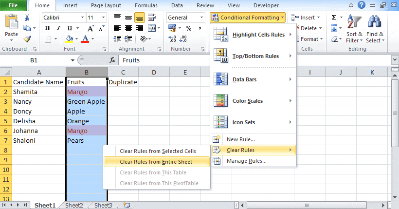
The steps to clear the existing rules (shown in the succeeding image) are listed as follows:
Step 1: In the Home tab, select “conditional formatting” from the “styles” section.
Step 2: In “clear rules” option, select either of the following:
- Clear rules from selected cells–This resets the rules for the selected range of the table. So, prior to clearing the rules, the data needs to be selected.
- Clear rules from entire sheet–This clears the rules for the entire sheet.
The blue highlighted cells disappear and the original table is displayed.
#4 – Remove Duplicates
Let us check and delete duplicate values from a selected range. Prior to deletion, keeping a copy of the table is advisable because the duplicates will be permanently deleted.
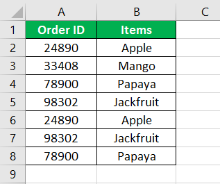
The following table displays a series of items with their corresponding IDs.
The steps to find and delete duplicate values are listed as follows:
Step 1: Select the range of the table whose duplicates are required to be deleted.
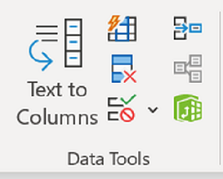
Step 2: In the Data tab, select “remove duplicates” from the “data tools” section.
Note: The “remove duplicates” option helps eliminate duplicates and retain unique cell values.
Step 3: The pop-up window titled “remove duplicates” appears, as shown in the succeeding image. By default, the following options are already selected:
- The checkboxes for both the headers (“order ID” and “items”)
- The “select all” box
Since the table consists of column headers, select the checkbox “my data has headers.” Click “Ok” to execute.
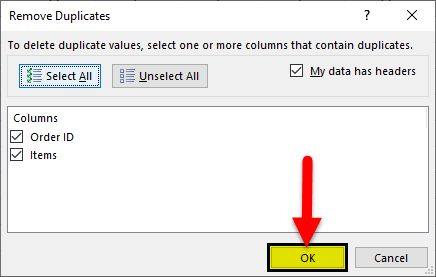
Note: To change the number of columns selected, click “unselect all.” Following this, the desired columns from which the duplicates are to be deleted can be selected.
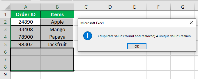
Step 4: The result is shown in the succeeding image. A prompt is displayed which states the following details:
- The number of duplicate values removed from the table
- The number of unique values that remain in the table after deletion
Click “Ok.” Hence, the duplicate values along with their corresponding rows are deleted.
#5 – COUNTIF Formula
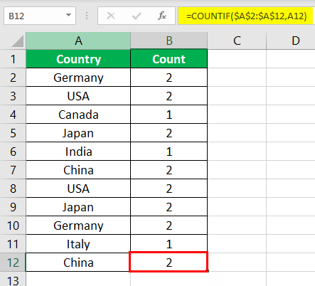
The following table displays the names of a few countries. We want to identify the duplicate values using the COUNTIF function.
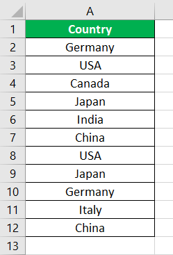
The COUNTIF function requires the range (column containing duplicate entries) and the cell criteria. It returns the number of corresponding duplicates for every cell.
The steps to find the duplicate values in excel with the help of the COUNTIF function are listed as follows:
Step 1: Enter the formula shown in the succeeding image. Press the “Enter” key.
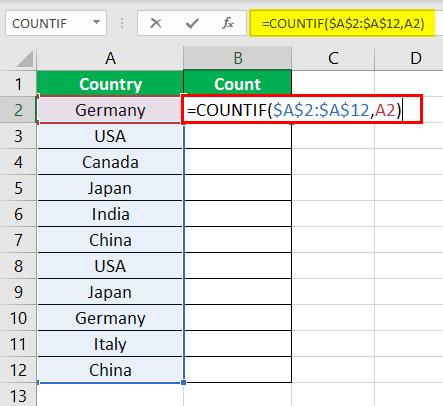
Note: The range must be fixed with the dollar ($) sign. Otherwise, the cell reference will change on dragging the formula.
Step 2: Drag the formula till the end of the table with the help of the fill handle. Alternatively, place the cursor on cell B2 and double-click the fill handle. The fill handle appears at the lower right corner of cell B2.
Step 3: The output of the formula is shown in the following image. It returns the count of duplicates for the entire data set.
Note: The filter can be applied to the column header to view the occurrences greater than one.
Frequently Asked Questions
1. What does it mean to find duplicates in Excel?
While consolidating different worksheets, several duplicates may be found in a data set. MS Excel helps to find and highlight such duplicates. It is also possible to filter a column for duplicate values.
An easy way to search for duplicates is by using the COUNTIF formula. This formula can count the total number of duplicates in a column. It can also count the number of individual instances of a particular duplicate entry. It accepts two arguments–the range and the criteria.
2. How to find duplicates in a column of Excel?
To check a column for duplicates, the formula is given as follows:
“=COUNTIF(A:A,A2)>1”
The formula checks for duplicates in column A. The topmost cell is A2. For every duplicate value, the formula returns “true.” For every unique value, the formula returns “false.”
Note: For an output other than “true” and “false,” the COUNTIF formula can be enclosed in the IF function.
3. What is the formula to find duplicates in Excel?
The generic formula to find the exact, case-sensitive duplicate values is stated as follows:
“IF(SUM((-EXACT(range,uppermost_cell)))<=1,””,”Duplicate”)”
The EXACT function compares the cell range with the target cell. The SUM function adds the number of instances. If the occurrence is greater than 1, the IF function returns “duplicate.”
Note 1: Since it is an array formula, it should be entered using “Ctrl+Shift+Enter.”
Note 2: If the same word appears twice in lowercase and once in uppercase, the formula will not count the uppercase word as duplicate.
Recommended Articles
This has been a guide to Find Duplicates in Excel. Here we discuss how to identify, check and show duplicates in excel with examples. You may also look at these useful functions in Excel –
- How to Use IF Formula in Excel (with Examples)?
- Conditional Formatting for Blank Cells | Steps
- Create a Dashboard in Excel
- Apply Conditional Formatting in Pivot Table
![]()
Download Article
![]()
Download Article
When working with a Microsoft Excel spreadsheet with lots of data, you’ll probably encounter duplicate entries. Microsoft Excel’s Conditional Formatting feature shows you exactly where duplicates are, while the Remove Duplicates feature will delete them for you. Viewing and deleting duplicates ensures that your data and presentation are as accurate as possible.
-
1
Open your original file. The first thing you’ll need to do is select all data you wish to examine for duplicates.
-
2
Click the cell in the upper left-hand corner of your data group. This begins the selecting process.
Advertisement
-
3
Hold down the ⇧ Shift key and click the final cell. Note that the final cell should be in the lower right-hand corner of your data group. This will select all of your data.
- You can do this in any order (e.g., click the lower right-hand box first, then highlight from there).
-
4
Click on «Conditional Formatting.« It can be found in the «Home» tab/ribbon of the toolbar (in many cases, under the «Styles» section).[1]
Clicking it will prompt a drop-down menu. -
5
Select «Highlight Cells Rules,» then «Duplicate Values.« Make sure your data is still highlighted when you do this. This will open a window with customization options in another drop-down menu.[2]
-
6
Select «Duplicate Values» from the drop-down menu.
- If you instead wish to display all unique values, you can select «Unique» instead.
-
7
Choose your highlight color. The highlight color will designate duplicates. The default is light red with dark red text.[3]
-
8
Click «OK» to view your results.
-
9
Select a duplicate’s box and press Delete to delete it. You won’t want to delete these values if each piece of data represents something (e.g., a survey).
- Once you delete a one-time duplicate, its partner value will lose its highlight.
-
10
Click on «Conditional Formatting» again. Whether you deleted your duplicates or not, you should remove the highlight formatting before exiting the document.
-
11
Select «Clear Rules,» then «Clear Rules from Entire Sheet» to clear formatting. This will remove the highlighting around any duplicates you didn’t delete.[4]
- If you have multiple sections of your spreadsheet formatted, you can select a specific area and click «Clear Rules from Selected Cells» to remove their highlighting.
-
12
Save your document’s changes. If you’re satisfied with your revisions, you have successfully found and deleted duplicates in Excel!


Advertisement
-
1
Open your original file. The first thing you’ll need to do is select all data you wish to examine for duplicates.
-
2
Click the cell in the upper left-hand corner of your data group. This begins the selecting process.
-
3
Hold down the ⇧ Shift key and click the final cell. The final cell is in the lower right-hand corner of your data group. This will select all of your data.
- You can do this in any order (e.g., click the lower right-hand box first, then highlight from there).
-
4
Click on the «Data» tab in the top section of the screen.
-
5
Find the «Data Tools» section of the toolbar. This section includes tools to manipulate your selected data, including the «Remove Duplicates» feature.
-
6
Click «Remove Duplicates.« This will bring up a customization window.
-
7
Click «Select All.« This will verify all of your columns have been selected.[5]
-
8
Check any columns you wish to use this tool on. The default setting has all columns checked.
-
9
Click the «My data has headers» option, if applicable. This will prompt the program to label the first entry in each column as a header, leaving them out of the deletion process.
-
10
Click «OK» to remove duplicates. When you are satisfied with your options, click «OK». This will automatically remove any duplicate values from your selection.
- If the program tells you that there aren’t any duplicates—especially if you know there are—try placing a check next to individual columns in the «Remove Duplicates» window. Scanning each column one at a time will resolve any errors here.
-
11
Save your document’s changes. If you’re satisfied with your revisions, you have successfully deleted duplicates in Excel!


Advertisement
Add New Question
-
Question
How do I get rid of colored highlighted areas in Excel?

Press Ctrl-H, click Options, and then click the top Format button to search for colored cells (using the Fill tab). Leave the «Replace with» field blank to delete the contents of cells with the format you specified.
-
Question
How can I tell if a motherboard or hard drive is bad in a PC?
Faulty hard drives will often have data that is said to be corrupted. Motherboards that are faulty result in hardware orientated failures.
-
Question
Can this method be used to find duplicates between several different sheets? If not, what method can I use to do that?
Kadriguler
Community Answer
The repeating data with count of repetitions can be found easily with Excel Vba.
Ask a Question
200 characters left
Include your email address to get a message when this question is answered.
Submit
Advertisement
wikiHow Video: How to Find Duplicates in Excel
-
You can also identify duplicate values by installing a third-party add-in utility. Some of these utilities enhance Excel’s conditional formatting feature to enable you to use multiple colors to identify duplicate values.
-
Deleting your duplicates comes in handy when reviewing attendance lists, address directories, or similar documents.
Thanks for submitting a tip for review!
Advertisement
-
Always save your work when you’re done!
Advertisement
References
About This Article
Article SummaryX
To view duplicate cells in your worksheet, start by highlighting the column or row you want to check. Click the Home tab, and then click the Conditional Formatting button in the «Styles» area of the toolbar. Select Highlight Cells Rules on the menu, and then Duplicate Values. Now, choose how you’d like Excel to highlight the duplicates in your data, such as in Light Red Fill with Dark Red Text or with a Red Border. Click OK to see your highlighted duplicates. When you’re finished, clear the special formatting by clicking the Conditional Formatting button and selecting Clear Rules and then Clear Rules from Entire Sheet. If you want to delete duplicates without viewing them first, select the cells you want to check, and then click the Data tab at the top. In the «Data Tool» area of the toolbar, click Remove Duplicates. Click the Select All button at the top-left corner of the window to select all columns, or just select the ones you want to check. Check the box to «My data has headers» if your column has a title cell at the top, and then click OK to remove duplicate cells from the selected area.
Did this summary help you?
Thanks to all authors for creating a page that has been read 1,808,322 times.
Reader Success Stories
-

Anna Krieger
Nov 30, 2016
«Thanks a lot for the functions, makes life much easier when getting a list of 1600 items and having to find whether…» more
Is this article up to date?
![]()
Find Duplicates in Excel

It is very easy to find duplicates in Excel. We can use built in tools (Conditional Formats, Filters) or formula (COUNTIF or VLOOKUP) to find duplicates in Excel Columns or Rows. Let us see the best and easy methods to find duplicate values in Excel.
Find duplicates Using Conditional Formatting
We can easily identify the duplicates using Conditional Formatting Tools in Excel. We can select the range and highlight the duplicate values with color. Following are the different methods to find duplicate entries in excel and strikethrough the duplicates using Conditional Formatting.
Highlighting duplicate values in Excel
We can highlight the duplicate values in the Excel with specific color. We can change the fill color and font color for the duplicate values. Please follow the below steps to identify the duplicates.
- Select the required range of cell to find duplicates
- Go to ‘Home’ Tab in the Ribbon Menu
- Click on the ‘Conditional Formatting’ command
- Go to ‘Highlight Cells Rules’ and Click on ‘Duplicate Values…’
- And Choose the formatting Options from the drop down list and Click on ‘OK’
Now you can see that all the duplicate values are highlighted as shown in the screen-shot.
Strike through duplicate values in Excel
We can strike through the duplicate values in the Excel. It is very helpful to strike out all duplicate entries in a range of cells. We can use the conditional formatting command in Excel to strike through the duplicate Cells.

- Select the required range of cell to strike through the duplicates
- Go to ‘Home’ Tab in the Ribbon
- Click on the ‘Conditional Formatting’ command
- Go to ‘Highlight Cells Rules’ and Click on ‘Duplicate Values…’
- And Choose the Custom Format from formatting Options from the drop down list
- Select the Strikethrough option from Font effects and Click on ‘OK’
Now you can see that all the duplicate values are stroked out as shown in the screen-shot.
Formula for checking duplicates
We can create formula using COUNTIF or VLOOKUP Functions to check the duplicates in Excel. Following is the step by explanation for finding duplicate values using Excel Formula.
Finding Duplicates using COUNTIF Formula
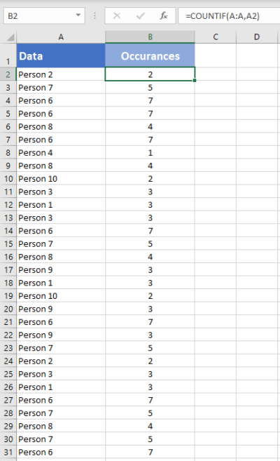
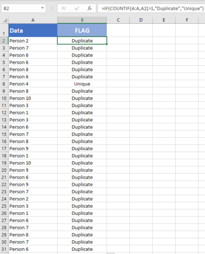
We can use COUNTIF Formula in Excel Cells to identify duplicates in Excel. COUNTIF formula helps to find duplicates in One Column, returns the number of occurrences of a given value. We can identify the duplicates if the Count is greater than 1. We can create new column to mark the duplicates using Excel COUNTIF Formula.
You can see that we have enter the COUNTIF formula in Range B2 to check the total occurrences of A1 value in the entire Column A:A.This will return the frequency of each Cell value of Column A in Column B.
We can identify the duplicate Cells based on the value in the Column B. If the values is greater than 1, we confirm that the values contains duplicate entries in the specified range or column.
Mark Duplicates and Unique Entries using Formula
We can enhance the above formula to mark all duplicates in a Column. The following formula will return ‘Duplicate’ if the cell value contains duplicate values, otherwise returns ‘Unique’.
=IF(COUNTIF(A:A,A2)>1,"Duplicate","Unique")
Formula will return ‘Duplicate’ in the Column B if the value repeats (count >1).
It will return ‘Unique’ in the Column B if the count is 1.
Find duplicate values in excel using VLookup
We can use VLOOKUP formula to compare two columns (or lists) and find the duplicate values. Vlookup helps to find duplicates in Two Column and duplicate rows based on Multiple Columns. Following are steps to find duplicates using VLOOKUP function.
We have two lists in the Excel List 1 in Column A and List 2 in Column B. Let us find the duplicate values in the List 2 which are part of List 1.
=VLOOKUP(B2,$A$2:$A$15,1,FALSE)
VLOOKUP Formula will check for the Cell B2 value in the specified Range (A2:A5) and Returns the value if found, it will return #NA if it is not found in List 1. We can confirm if the the value is duplicated in List 1 and 2 if it returns the Value, it will be unique if it returns #NA.

How to find duplicate values in Excel using VlookUp?
You can use Excel formula to find the duplicate values in Excel by using vlookup formula as described below. You can use the Excel VlookUp to identify the duplicates in Excel.
=IF(ISNA(VLOOKUP(B2,$A$2:$A$15,1,FALSE)),"Unique","Duplicate")
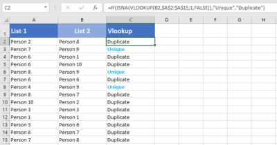
We can enhance this formula to identify the duplicates and unique values in the Column 2. We can use the Excel IF and ISNA Formulas along with VLOOKUP to return the required Labels.
You can use this method to compare with other worksheets and find duplicate values in Different Excel Sheets.
How to find duplicate values in two columns in excel using VlookUp?
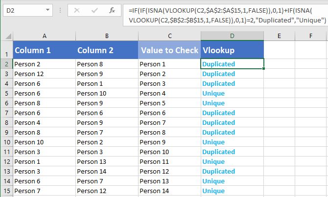
Follow the below steps to find the duplicate values in two columns in excel using VlookUp. We generally need this to compare two columns and check if a value is existing in two columns.
=IF(IF(ISNA(VLOOKUP(C2,$A$2:$A$15,1,FALSE)),0,1)
+IF(ISNA(VLOOKUP(C2,$B$2:$B$15,1,FALSE)),0,1)=2,"Duplicated","Unique")
Here, we have Two Target Columns A and B , we check if the items in Column C are duplicated or not.
If you wants to compare two columns and check for values are repeated in both the columns or not, you can use this formula.
Share This Story, Choose Your Platform!
2 Comments
-
Guru
August 12, 2019 at 7:45 pm — ReplyThanks for very useful instructions to check duplicates in Excel.
-
Tom
August 12, 2019 at 7:48 pm — ReplyThis is very clear and simple! Thanks a lot for providing clear help to identify the duplicates in Excel.
© Copyright 2012 – 2020 | Excelx.com | All Rights Reserved
Page load link
When you are working on a large number of data then you will encounter a few duplicate entries.
Sometimes these duplicate values are very useful but many times you want to remove the duplicate data. If you have 1000 data then it becomes quite difficult to find and remove the duplicate data.
Here we have provided the step-by-step process on how to find duplicates in excel.
Take a look and follow the process.
There are many ways to find duplicate items and values in excel. You might be thinking as to why should I apply any formula or method to find duplicate values as it is easy.
But it’s not about few data, you can apply a formula or method when you have lots of data.
The method or formula to find and remove the duplicate items make the process easier and saves your time. Here you can check three different processes.
1. Find Duplicates in Excel using Conditional Formatting
To find duplicate values in Excel, you can use conditional formatting excel formula, Vlookup, and Countif formula. After finding out the duplicate values, you can remove them if you want by using different methods that are described below.

Remove duplicate values
- Select all the duplicate cells or highlighted cells
- Delete the values by pressing the Delete button.
- After deleting the values, go to the conditional formatting.
- Choose Clear rules.
- And then choose clear rules from an entire sheet.
Another way to remove the duplicate value
This method will delete all the duplicate data permanently. If you want the duplicate data again, then copy the data on another worksheet.
- Select the cells on which you want to find and remove the duplicate values.
- Go to the ribbon and find the data option.
- In the data tab, you will find the remove duplicates option.

- Now check or uncheck the column on which you want to apply this constraint.
- Then click OK.

2. Find Duplicates in One Column using COUNTIF
Another way to detect duplicates is via the COUNTIF function. If you want to apply the COUNTIF function then check here how to find duplicates in Excel using the Excel COUNT function.
- If you have the list of items from where you want to find duplicates, then you need to apply the COUNTIF formula to it.
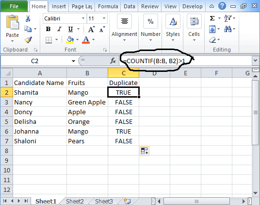
- The syntax for COUNTIF: “=COUNTIF(B:B, B2)>1”.

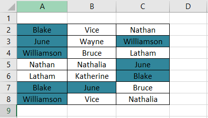
- In column A, you have the Buyer’s name and in column B, you have the fruits name that he or she likes. Now you want to find the duplicate items.
- Put this COUNTIF formula in column C.
- For all duplicate fields, it shows TRUE whereas, for non-duplicate fields, it shows FALSE.
- Now by following the above step-by-step process, you can delete all the duplicate items that you do not need.
Find Duplicates in Two Columns in Excel
Above we have seen how to find duplicate values in one column, now we will see here how to find duplicates in two columns in excel.
In this example, we have taken a table where the candidate name is in column A and Fruits is in column B. Now we want to find duplicate values having the same name and fruits.
The formula to find duplicate values in two columns is
=If (Countifs($A$2:$A$8, $A2, $B$2:$B$8, $B2)>1, "Duplicate Values"," ")
How to Count Duplicates in Excel
If you want to know the total number of duplicate values then you need to use the Count function. For counting duplicate values you need to use the countif formula.
=Countif($A$2:$A$8, $A2)
3. Filter Duplicates in Excel
Another method to find duplicates in excel is to filter data to get duplicate values.
Remove Duplicates Online
To remove duplicates, you need to follow the below-mentioned process
- Select the table by dragging the mouse.
- Right-click on the table.
- Delete the row by choosing the Delete Row option.
Highlight Duplicates in Excel
In order to highlight the duplicate values, you can either use a conditional formula to find duplicates in excel or follows the below-mentioned process.
- Select the duplicate values.
- Go to the Fill color option and select the color.


- This will highlight the duplicate values in excel.
Apart from these, there are other processes available by which you can find the duplicate items available in your data set. After finding out the duplicate values, you can remove them easily. Stay connected with our website to know other Excel features.
Related Queries
Here we have listed a few queries that are asked by Excel learners. If you are also facing this kind of problem then you can check it here.
Q1. How to delete duplicate e-mail addresses if you have 10,000 emails in your data set?
Ans. If you have all email addresses in a single column then select the column and go to the “Data” ribbon. You will find the ‘Remove Duplicates’ tab in data tools.
Click on Remove Duplicates and you will find another dialog box where you need to make a selection. Press Ok and you receive the unique email addresses.
Q2. How to find the repeated teacher’s name in Column A? The data is
- B1= Maths/English Jasmine, Eon
- B2= Physics Johana
- B3= History Poole
- B4= English/Physics Sam, Jasmine
- B5= Chemistry Romeo
Ans. To solve this problem, create three separate columns. In the first column, mention the class name. In the second column, put the teacher’s name, and in the third mention another teacher’s name. Now in the fourth column, put the formula =COUNTIF(B:B,B1)>1
Using this formula, you will find “TRUE” if the value is duplicate.
Q3. How to sort data before applying a filter?
Ans. To sort data you need to choose the Sort tab in excel. Sorting a data set is quite an easy process. Follow the process mentioned below and sort your data completely.
- Select the data set.
- Go to the Data ribbon.
- In the Sort & Filter section, you will find the Sort icon. Click on the icon and sort your data.
Q4. How to compare two columns in excel?
This question was mainly asked by the interviewer at the time of the interview. There are many ways to compare the two columns:
- =A2=B2 This is the simple formula used to compare two columns.
- Conditional Formatting: In this, you need to follow the above process, you can check the conditional formatting excel link to get detailed information.
- Vlookup: You can also use the Vlookup formula to compare two columns using Vlookup for research, ISNA for performance, and If to customize the result.
- Excel If Statement: This is a quite useful function in excel and it can be used in many ways. To get the detailed information Click Here.
Q5. How to filter data in excel?
Filtering in Excel is an easy process. In the sort & filter section, you will find the Filter icon. Click on the icon and filter your data.
In this tutorial, we have covered all the excel topics that are best for beginners and experts. We always try to solve all the problems that people face while working on excel. If you have any other query or want to ask something then you can mention in the comment box below. One of our team members will be back with the answer.
You may also like the following Excel tutorials:
- How to Remove Formulas in Excel (and keep the data)
- How to Fill Blank Cells with Value above in Excel
- How to Generate Random Numbers in Excel (Without Duplicates)
- How to Find Merged Cells in Excel
- Highlight Cell If Value Exists in Another Column in Excel
- Using Conditional Formatting with OR Criteria in Excel
- How to Remove Duplicate Rows based on one Column in Excel?
- Get Unique Values from a Column in Excel
- How to Count Unique Values in Excel (Formulas)
- How to Use Greater Than or Equal to Operator in Excel Formula?