
In Excel for the web, you can view the results of a regression analysis (in statistics, a way to predict and forecast trends), but you can’t create one because the Regression tool isn’t available.
You also won’t be able to use a statistical worksheet function such as LINEST to do a meaningful analysis because it requires you enter it as an array formula, which isn’t supported in Excel for the web.
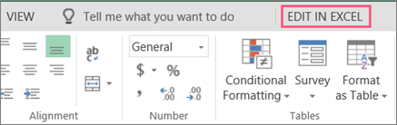
If you have the Excel desktop application, you can use the Open in Excel button to open your workbook and use either the Analysis ToolPak’s Regression tool or statistical functions to perform a regression analysis there.
Click Open in Excel and perform a regression analysis.
For news about the latest Excel for the web updates, visit the Microsoft Excel blog.
For the full suite of Office applications and services, try or buy it at Office.com.
Need more help?
Want more options?
Explore subscription benefits, browse training courses, learn how to secure your device, and more.
Communities help you ask and answer questions, give feedback, and hear from experts with rich knowledge.
Regression is done to define relationships between two or more variables in a data set. In statistics, regression is done by some complex formulas. But, Excel has provided us with tools for regression analysis. So, in the Excel Analysis ToolPak, click “Data Analysis” and “Regression” to conduct regression analysis in Excel.
Table of contents
- What is Regression Analysis in Excel?
- Explained
- Examples
- How to Run Regression Analysis Tool in Excel?
- How to Use Regression Analysis Tool in Excel?
- Steps to Create Regression Chart in Excel
- Things to Remember
- Recommended Articles
Explained
The Regression analysis tool performs linear regression in excelLinear Regression is a statistical excel tool that is used as a predictive analysis model to examine the relationship between two sets of data. Using this analysis, we can estimate the relationship between dependent and independent variables.read more examination using the “minimum squares” technique to fit a line through many observations. You can examine how an individual dependent variable is influenced by the estimations of at least one independent variable. For instance, you can investigate how such factors influence a sportsman’s performance as age, height, and weight. You can distribute shares in the execution measure to every one of these three components, given a lot of execution information, and then utilize the outcomes to foresee the execution of another person.
The Excel regression analysis tool helps you see how the dependent variable changes when one of the independent variables fluctuates and permits you to numerically figure out which of those variables truly has an effect.
Examples
- Sales of shampoo are dependent upon the advertisement. If $1 million increases advertising expenditure, sales will be expected to increase by $23 million. If there were no advertising, we would expect sales without any increment.
- House sales (selling price, number of bedrooms, location, size, design) predict the selling price of future sales in the same area.
- Soft drink sales massively increase in summer when the weather is too hot. People purchase more and more soft drinks to keep them cool. The higher the temperature, the higher the sales and vice versa.
- In March, exam season started, and sales increased due to students purchasing exam pads. Exam pads sale depends upon the examination season.
How to Run Regression Analysis Tool in Excel?
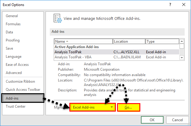
- We must enable the Analysis ToolPak Add-in.
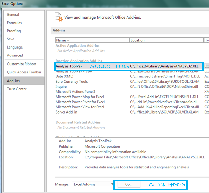
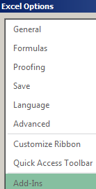
- In Excel, click on the “File” on the extreme left-hand side, go and click on the “Options” at the end.

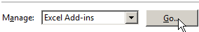
- On clicking on “Options,” select “Add-ins” on the left side. Excel Add-ins are chosen in the “View and manage Microsoft Add-ins” and “Manage” boxes. Then, click “Go.”

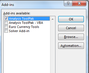
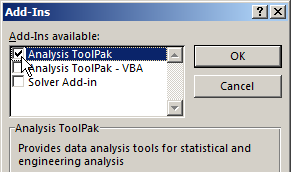
- In the Add-in dialog box, click on Analysis Toolpak, and click OK:

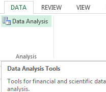
It will add the “Data Analysis” tools on the right-hand side to the Excel ribbon’s “Data” tab.


How to Use Regression Analysis Tool in Excel?
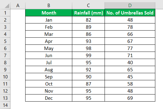
We must use the data for regression analysis in Excel.
You can download this Regression Excel Template here – Regression Excel Template
Once Analysis ToolpakExcel’s data analysis toolpak can be used by users to perform data analysis and other important calculations. It can be manually enabled from the addins section of the files tab by clicking on manage addins, and then checking analysis toolpak.read more is added and enabled in the Excel workbook, follow the steps mentioned below to practice the analysis of regression in Excel:
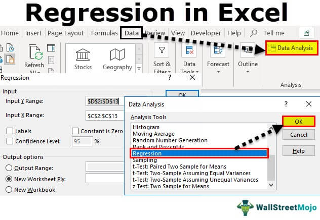
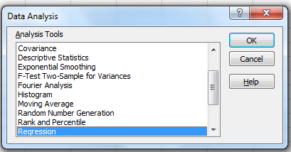
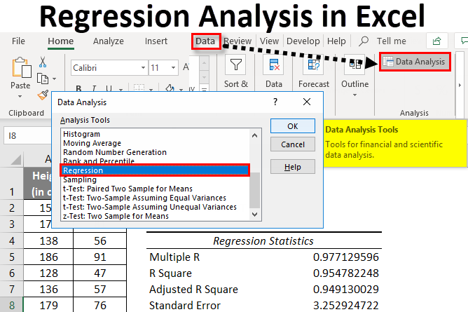
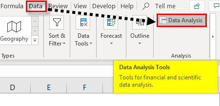
- Step 1: On the Data tab in the Excel ribbonThe ribbon is an element of the UI (User Interface) which is seen as a strip that consists of buttons or tabs; it is available at the top of the excel sheet. This option was first introduced in the Microsoft Excel 2007.read more, click the Data Analysis

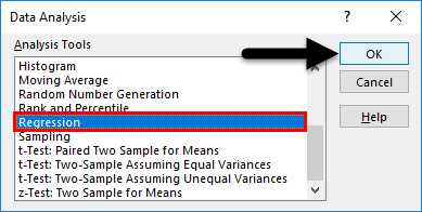
- Step 2: Click on the “Regression” and click “OK” to enable the function.

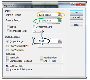
- Step 3: On clicking the “Regression“ dialog box, we must arrange the accompanying settings:
- For the dependent variable, select the “Input Y Range,” which denotes the dependent data. Here, in the below-given screenshot, we have selected the range from $D$2:$D$13.

- Select the “Input X Range,” which denotes the independent data for the independent variable. Here, in the below-given screenshot, we have selected the range from $C$2:$C$13.

- Step 4: Click “OK” and analyze the data accordingly.

When you run the regression analysis in Excel, the following output will come:


You can also make a scatter plot in excelScatter plot in excel is a two dimensional type of chart to represent data, it has various names such XY chart or Scatter diagram in excel, in this chart we have two sets of data on X and Y axis who are co-related to each other, this chart is mostly used in co-relation studies and regression studies of data.read more of these residuals.
Steps to Create Regression Chart in Excel
- Step 1: Select the data as given in the below screenshot.

- Step 2: Tap on the “Inset” tab. In the “Charts” gathering, tap the “Scatter” diagram or some other as a required symbol. Select the chart which suits the information.

- Step 3: We can modify the chart when required and fill in the hues and lines of your decision. For instance, we can pick alternate shading and utilize a strong line of a dashed line. We can customize the graph as we want to customize it.

Things to Remember
- We must always check the dependent and independent values. Otherwise, the analysis will be wrong.
- If you test a huge number of data and thoroughly rank them based on their validation period statisticsStatistics is the science behind identifying, collecting, organizing and summarizing, analyzing, interpreting, and finally, presenting such data, either qualitative or quantitative, which helps make better and effective decisions with relevance.read more.
- Choose the data carefully to avoid any kind of error in excel analysis.
- We can optionally check any of the boxes at the bottom of the screen, although none of these is necessary to obtain the line best-fit formula.
- Start practicing with small data to understand the better analysis and run the regression analysis tool in Excel easily.
Recommended Articles
This article is a step-by-step guide to Regression Analysis in Excel. Here we discuss how to run regression in Excel, its interpretation, and use this tool along with Excel examples and downloadable Excel templates. You may also look at these useful functions in Excel: –
- Examples of Normal Distribution Graph in Excel
- Regression vs. ANOVABoth the Regression and ANOVA are the statistical models which are used in order to predict the continuous outcome but in case of the regression, continuous outcome is predicted on basis of the one or more than one continuous predictor variables whereas in case of ANOVA continuous outcome is predicted on basis of the one or more than one categorical predictor variables.read more
- Excel Exponential Smoothing
- Exponential Function ExcelExponential Excel function(EXP) is an inbuilt function in excel used to calculate the exponent raised to the power of any number you provide. In this function the exponent is constant and is also known as the base of the natural algorithm.read more
Reader Interactions
To run the regression, arrange your data in columns as seen below. Click on the “Data” menu, and then choose the “Data Analysis” tab. You will now see a window listing the various statistical tests that Excel can perform. Scroll down to find the regression option and click “OK”.
Contents
- 1 Can Excel perform regression analysis?
- 2 How do you calculate regression analysis?
- 3 What is a regression equation example?
- 4 How do you write a regression equation?
- 5 How do you perform a regression analysis manually?
- 6 How do you get data analysis on Excel?
- 7 How do you do a regression in Excel with multiple variables?
- 8 How do you do linear regression?
- 9 How do you do regression?
- 10 How do you find b1 and b0 in Excel?
- 11 How do you find b0 and b1?
- 12 Is Excel good for data analysis?
- 13 Can Excel be used for statistical analysis?
- 14 Is Excel a data analysis tool?
- 15 What is the formula for multiple linear regression?
Can Excel perform regression analysis?
You can use Excel’s Regression tool provided by the Data Analysis add-in.Tell Excel that you want to join the big leagues by clicking the Data Analysis command button on the Data tab. When Excel displays the Data Analysis dialog box, select the Regression tool from the Analysis Tools list and then click OK.
How do you calculate regression analysis?
Regression analysis is the analysis of relationship between dependent and independent variable as it depicts how dependent variable will change when one or more independent variable changes due to factors, formula for calculating it is Y = a + bX + E, where Y is dependent variable, X is independent variable, a is
What is a regression equation example?
A regression equation is used in stats to find out what relationship, if any, exists between sets of data. For example, if you measure a child’s height every year you might find that they grow about 3 inches a year. That trend (growing three inches a year) can be modeled with a regression equation.
How do you write a regression equation?
The Linear Regression Equation
The equation has the form Y= a + bX, where Y is the dependent variable (that’s the variable that goes on the Y axis), X is the independent variable (i.e. it is plotted on the X axis), b is the slope of the line and a is the y-intercept.
How do you perform a regression analysis manually?
Simple Linear Regression Math by Hand
- Calculate average of your X variable.
- Calculate the difference between each X and the average X.
- Square the differences and add it all up.
- Calculate average of your Y variable.
- Multiply the differences (of X and Y from their respective averages) and add them all together.
How do you get data analysis on Excel?
Windows
- Click the File tab, click Options, and then click the Add-Ins category.
- In the Manage box, select Excel Add-ins and then click Go.
- In the Add-Ins box, check the Analysis ToolPak check box, and then click OK. If Analysis ToolPak is not listed in the Add-Ins available box, click Browse to locate it.
How do you do a regression in Excel with multiple variables?
In Excel you go to Data tab, then click Data analysis, then scroll down and highlight Regression. In regression panel, you input a range of cells with Y data, with X data (multiple regressors), check the box with output range or new worksheet, and check all the plots that you need.
How do you do linear regression?
A linear regression line has an equation of the form Y = a + bX, where X is the explanatory variable and Y is the dependent variable. The slope of the line is b, and a is the intercept (the value of y when x = 0).
Use Regression to Analyze a Wide Variety of Relationships
- Model multiple independent variables.
- Include continuous and categorical variables.
- Use polynomial terms to model curvature.
- Assess interaction terms to determine whether the effect of one independent variable depends on the value of another variable.
How do you find b1 and b0 in Excel?
Use [email protected] =LINEST(ArrayY, ArrayXs) to get b0, b1 and b2 simultaneously.
How do you find b0 and b1?
Formula and basics
The mathematical formula of the linear regression can be written as y = b0 + b1*x + e , where: b0 and b1 are known as the regression beta coefficients or parameters: b0 is the intercept of the regression line; that is the predicted value when x = 0 . b1 is the slope of the regression line.
Is Excel good for data analysis?
Excel is a great tool for analyzing data. It’s especially handy for making data analysis available to the average person at your organization.
Can Excel be used for statistical analysis?
Excel offers a wide range of statistical functions you can use to calculate a single value or an array of values in your Excel worksheets. The Excel Analysis Toolpak is an add-in that provides even more statistical analysis tools.
Is Excel a data analysis tool?
The Analysis ToolPak is an Excel add-in program that provides data analysis tools for financial, statistical and engineering data analysis.
What is the formula for multiple linear regression?
Since the observed values for y vary about their means y, the multiple regression model includes a term for this variation. In words, the model is expressed as DATA = FIT + RESIDUAL, where the “FIT” term represents the expression 0 + 1x1 + 2x2 +xp.
Regression is an Analysis Tool, which we use for analyzing large amounts of data and making forecasts and predictions in Microsoft Excel.
Want to predict the future? No, we are not going to learn astrology. We are into numbers and we will learn regression analysis in Excel today.
To predict future estimates, we will study:
- REGRESSION ANALYSIS USING EXCEL FUNCTIONS (MANUAL REGRESSION FINDING)
- REGRESSION ANALYSIS USING EXCEL’S ANALYSIS TOOLPAK ADD-IN
- REGRESSION CHART IN EXCEL
Let’s do it…
Scenario:
Let’s assume you sell soft drinks. How cool will it be if you can predict:
- How many soft drinks will be sold next year based on previous year’s data?
- Which fields need to be focused?
- And how can you increase your sales by changing your strategy?
It will be profitably awesome. Right?… I know. So let’s get started.
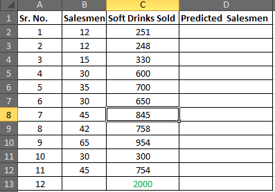
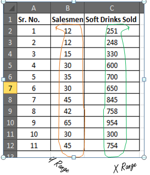
You have 11 records of salesmen and soft drinks sold.
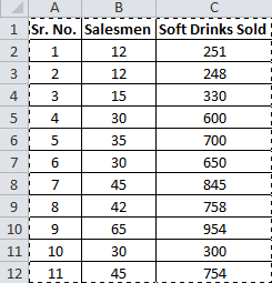
Now based on this data you want to predict the number of salesmen required to achieve 2000 sales of soft drinks.

The regression equation is a tool to make such close estimates. To do so, we need to know Regression first.
REGRESSION ANALYSIS USING EXCEL FUNCTIONS (MANUAL REGRESSION FINDING)
This part will make you understand regression better than just telling excel regression procedure.
Introduction:
Simple Linear Regression:
The study of the relationship between two variables is called Simple Linear Regression. Where one variable depends on the other independent variable. The dependent variable is often called by names such as Driven, Response, and Target variable. And the independent variable is often pronounced as a Driving, Predictor or simply Independent variable. These names clearly describe them.

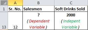
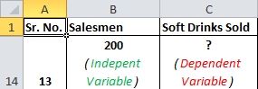
Now let’s compare this with your scenario. You want to know the number of salesmen required to achieve 2000 sales. So here, the dependent variable is the number of salesmen and the independent variable is sold soft drinks.
The independent variable is mostly denoted as x and dependent variable as y.
In our case, soft drinks are sold x and the number of salesmen is y.
If we want to know how many soft drinks will be sold if we appoint 200 salesmen, then the scenario will be vice-versa.
Moving On.
The “Simple” Math of Linear Regression Equation:
Well, it’s not simple. But Excel made it simple to do.
We need to predict the required number of salesmen for all 11 cases to get the 12th closest prediction.
Let’s say:
Soft Drink Sold is x
The number of Salesmen is y
The predicted y (number of salesmen) also called Regression Equation, would be
Now you must be wondering where the stat will you get the slope and intercept. Don’t worry, excel has functions for them. You do not need to learn how to find the slope and intercept it manually.
If you want, I will prepare a separate tutorial for that. Let me know in the comments section. These are some important data analytics tools.
Now let’s step into our calculation:
Step1: Prepare this small table
Step 2: Find the slope of the regression line
Excel Function for slopes is
=SLOPE(known_y’s,known_x’s)
Your known_y’s are in range B2:B12 and known_x’s are in range C2:C12

In cell B16, write the formula below
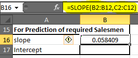
(Note: Slope is also called coefficient of x in the regression equation)
You will get 0.058409. Round up to 2 decimal digits and you will get 0.06.
Step 3: Find the Intercept of Regression Line
Excel function for the intercept is
=INTERCEPT(known_y’s, known_x’s)
We know what our known x’s and y’s
In cell B17, write down this formula

=INTERCEPT(B2:B12, C2:C12)
You will get a value of -1.1118969. Roundup to 2 decimal digits. You will get -1.11.
Our Linear Regression Equation is = x*0.06 + (-1.11). Now we can predict possible y depending on the target x easily.
Step 4: In D2 write the formula below
=C2*$B$16+$B$17 (Regression Equation)
You will get a value of 13.55.
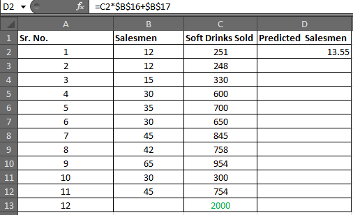
Select D2 to D13 and press CTRL+D to fill down the formula in the range D2:D13
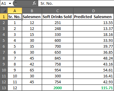
In cell D13 you have your required number of salesmen.
Hence, to achieve the target of 2000 Soft Drink Sales, you need an estimate of 115.71 salesmen or say 116 since it is illegal to cut humans into pieces.
Now using this you can easily conduct What-If analysis in excel. Just change the number of sales and it will show you many salesmen will it take to get that sales target achieved.
Play around it to find out:
How much workforce do you need to increase sales?
How many sales will increase if you increase your salesmen?
Make Your Estimate More Reliable:
Now you know that you need 116 salesmen to get 2000 sales done.
In analytics, nothing is just said and believed. You must give a percentage of reliability on your estimate. It is like giving a certificate of your equation.

Correlation Coefficient Formula:
The next thing you will be asked is how much these two variables are related. In static terms, you need to tell the coefficient of correlation.
Excel function for correlation is
In your case, known_x’s and Know_y’s are array1 and array2 irrespectively.
In B18 enter this formula
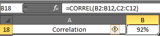
You will have 0.919090. Formate cell B2 into the percentage. Now have 92% of correlation.
Now, what this 92% means. It means, there 92% of chances of sales increase if you increase the number of salesmen and 92% of sales decrease if you decrease the number of salesmen. It is called Positive Correlation Coefficient.
R Squire (R^2) :
R Squire value tells you, by what percentage your regression equation is not a fluke. How much it is accurate by the data provided.
The Excel function for R squire is RSQ.
RSQ(known_y’s, Known_x’s)
In our case, we will get R squire value in cell B19.
In B19 enter this formula

So we have 84% of r Square value. Which is a very good explanation of our regression. It says that 84% of our data is just not by chance. Y (number of salesmen) is very much dependent on X (sales of soft drinks).
There are many other tests we can do on this data to ensure our regression. But manually it will be a complex and lengthy procedure. That is why excel provides Analysis Toolpak. Using this tool we can do this regression analysis in seconds.
REGRESSION IN EXCEL USING EXCEL’S ANALYSIS TOOLPAK ADD-IN
If you already know what regression equations are, and you just want your results quickly then this part is for you. But if you want to understand regression equations easily then scroll up to REGRESSION ANALYSIS USING EXCEL FUNCTIONS (MANUAL REGRESSION FINDING).
Excel provides a whole bunch of tools for analysis in its Analysis Toolpak. By default, it is not available in the Data tab. You need to add it. So let’s add it first.
Adding Analysis Toolpak to Excel 2016
If you don’t know where is data analysis in excel follow these steps
Step 1: Go to Excel Options: File? Options? Add-Ins
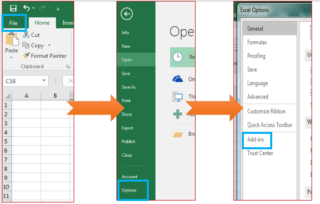
Step 2: Click on Add-Ins. You will see a list of available add-Ins.
Select Analysis ToolPak and at the bottom of the window, find manage. In manage select Excel Add-Ins and Click on GO.
Add-ins window will open. Here, select Analysis ToolPak. Then click the ok button.
Now you can access all functions of data analysis ToolPak from Data Tab.
Using Analysis ToolPak for Regression
Step 1: Go to the Data tab, Locate Data Analysis. Then click on it.

A dialogue box will pop up.
Step 2: Find ‘Regression’ in Analysis Tools list and hit the OK button.
The regression input window will pop up. You will see a number of available input options. But for now, we will just concentrate on Y Range and X Range, leaving everything else to default.

Step 4: Provide Inputs:
No. of Salesmen is Y
Sales of soft drinks are X
Hence
- Y Range= B2:B11
And
- X Range = C2:C11
For the output range, I have selected E4 on the same sheet. You may select a new worksheet to get results on a new worksheet in the same workbook or a complete new workbook. When you are done with your inputs, hit the OK button.
Results:
You will be served with a variety of information from your data. Don’t get overwhelmed. You don’t need to consume all the dishes.
We will only deal with those results which will help us to estimate the required number of salesmen
Step 5: We know the regression equation for estimation of y, that is
x*Slope+Intercept
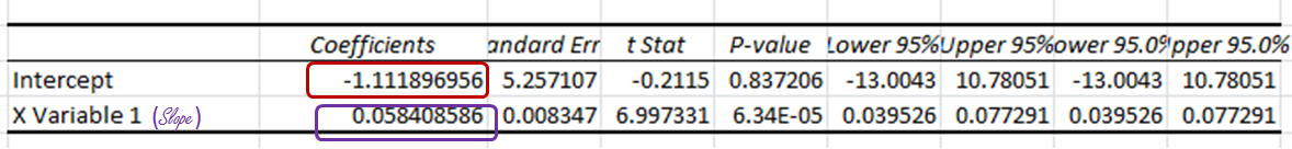
We just need to locate Slope and Intercept in results.
And here they are.
The intercept Coefficient is clearly mentioned.
The slope is written as ‘X Variable 1’, some times also mentioned as the coefficient of X. Round up them and we will get -1.11 as Intercept and 0.06 as Slope.
Step 6: From results, we can drive the Regression equation. And that would be
=x*(0.06) + (-1.11)
Prepare this table in excel.

For now, x is 2000, which is in cell E2.
In Cell F2 enter this formula
=E2*F21+F20
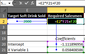
You will get a result of 115.7052757.

Rounding it up will give us 116 of Required Salesmen.
So we have learned how to form the regression equation manually and using Analysis ToolPak. How can you use this equation to estimate future stats?
Now let’s understand the regression output given by Analysis Toolpak.
Understanding the Regression Output:
There is no benefit, if you do regression analysis using analysis tool pack in excel and can’t interpret its meaning.
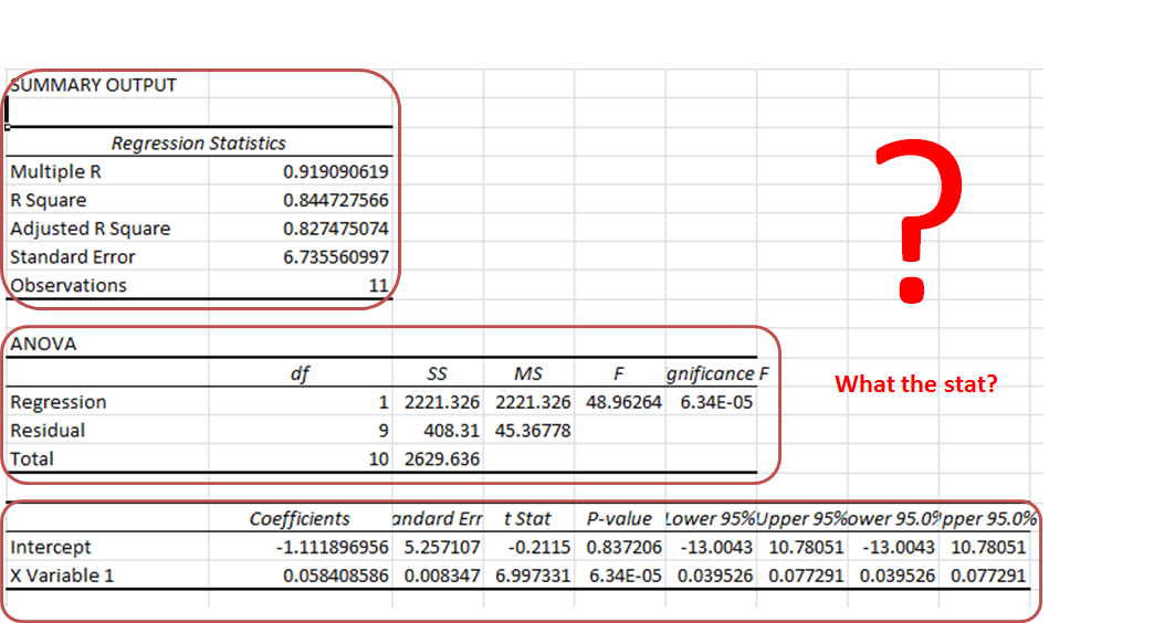
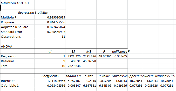
Summary Section:
As the name suggests, it is a summary of the data.

-
- Multiple R: It tells how fit the regression equation is to the data. It is also called the correlation coefficient.
In our case, it is 0.919090619 or 0.92 (roundup). This means that there is a 92% chance of an increase in sales if we increase our salesmen count.
-
- R Square: It tells the reliability of found regression. It tells us how many observations are part of our line of regression. In our case, it is 0.844727566 or 0.85. It means that our regression is fit by 85%.
- Adjusted R Square: Theadjusted square is just a more testified version of R square. Mainly useful in Multiple Regression Analysis.
- Standard Error: While R. Squire tells you how many data points fall near the regression line, the standard error tells you how far a data point can go from the regression line.
In our case, it is 6.74.
- Observation: This is simply the number of observations, which is 11 in our example.
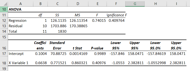
Anova Section:
This section is hardly used in linear regression.
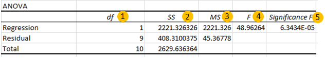
- df. It is a degree of freedom. It is used when calculating regression manually.
- SS. Sum of squares. It is just a sum of squares of variances. Used to find R squire values.
- MS. This means squared value.
- And 5. F and Significance of F. If the significance of F (p-value of the slope) is less than the F test than you can discard the null hypothesis and prove your hypothesis. In simple language, you can conclude that there is some effect of x on y when changed.
In our case, F is 48.96264 and Significance of F is 0.000063. It means our regression fits the data.
Regression Section:
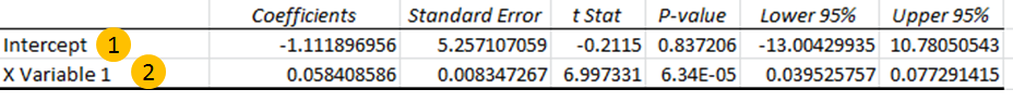
In this section, we have the two most important values for our regression equation.
- Intercept: We have an intercept here that tells where x-intercepts on Y. This is an important part of the regression equation. It is -1.11 in our case.
- X variable 1 (Slope). Also called the coefficient of x. It defines the tangent of the regression line.
REGRESSION CHART IN EXCEL
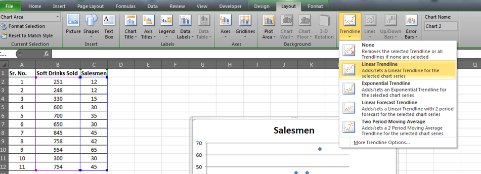
In excel, it is easy to plot a regression chart. Just follow these steps. To add Regression Chart in Excel 2016, 2013, and 2010 follow these simple steps.
Step 1. Have your known x’s in the first column and know y’s in the second.
In our case, we know Known_ x’s are Soft Drinks Sold. And known_y’s are Salesmen.

Step 2. Select your known x’s and y’s range.

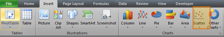
Step 3: Go to the Insert tab and click on the scatter chart.
You will have a chart that looks like this.
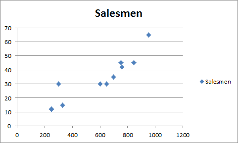
Step 4. Add the trend line: Goto layout and locate the trendline option in the analysis section.
Under the Trendline option, click on Linear Trendline.
You will have your graph looking like this.
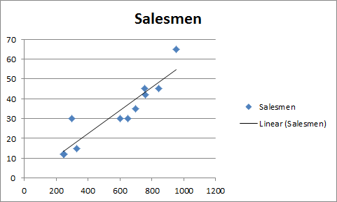
This is your regression graph.
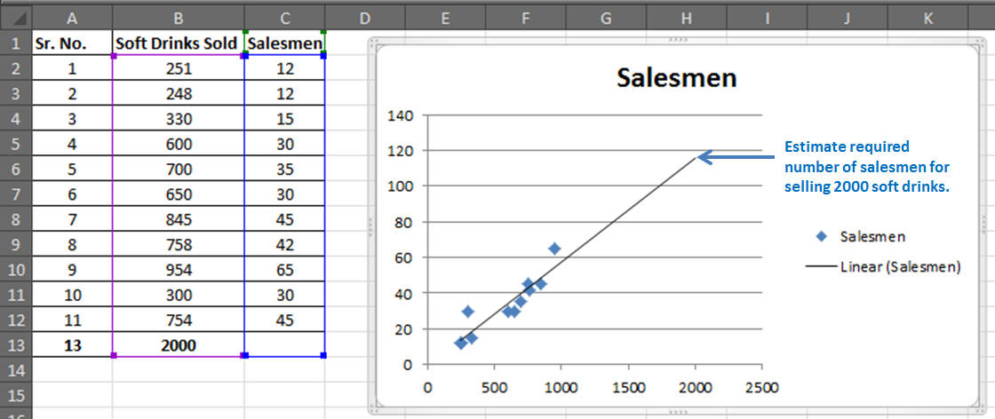
Now if you add the data below and extend the selected data. You will see a change in your graph.
For our example, we added 2000 to the Soft Drink Sold and left the Salesmen blank. And when we extend the range of the graph, this is what we will have.
It will give the required number of salesmen for doing 2000 sales of soft drinks in graphical form. Which is slightly below 120 in the graph. And from our regression equation, we know it is 116.

In this article, I tried to cover everything under Excel Regression Analysis. I explained regression in excel 2016. Regression in excel 2010 and excel 2013 is same as in excel 2016.
For any further query on this topic, use the comments section. Ask a question, give an opinion or just mention my grammatical mistakes. Everything is welcome. Just don’t hesitate to use the comment section.
Related Data:
How to Use STDEV Function in Excel
How To Calculate MODE function in Excel
How To Calculate Mean function in Excel
How to Create Standard Deviation Graph
Descriptive Statistics in Microsoft Excel 2016
How to Use Excel NORMDIST Function
How to use the Pareto Chart and Analysis
Popular Articles:
50 Excel Shortcut to Increase Your Productivity
How to use the VLOOKUP Function in Excel
How to use the COUNTIF function in Excel 2016
How to use the SUMIF Function in Excel
![]()
Download Article
![]()
Download Article
Regression analysis can be very helpful for analyzing large amounts of data and making forecasts and predictions. To run regression analysis in Microsoft Excel, follow these instructions.
-

1
If your version of Excel displays the ribbon (Home, Insert, Page Layout, Formulas…)
- Click on the Office Button at the top left of the page and go to Excel Options.
- Click on Add-Ins on the left side of the page.
- Find Analysis tool pack. If it’s on your list of active add-ins, you’re set.
- If it’s on your list of inactive add-ins, look at the bottom of the window for the drop-down list next to Manage, make sure Excel Add-Ins is selected, and hit Go. In the next window that pops up, make sure Analysis tool pack is checked and hit OK to activate. Allow it to install if necessary.
-
2
If your version of Excel displays the traditional toolbar (File, Edit, View, Insert…)
- Go to Tools > Add-Ins.
- Find Analysis tool pack. (If you don’t see it, look for it using the Browse function.)
- If it’s in the Add-Ins Available box, make sure Analysis tool pack is checked and hit OK to activate. Allow it to install if necessary.
Advertisement
-
3
Excel for Mac 2011 and higher do not include the analysis tool pack. You can’t do it without a different piece of software. This was by design since Microsoft does not like Apple.


Advertisement
-
1
Enter the data into the spreadsheet that you are evaluating. You should have at least two columns of numbers that will be representing your Input Y Range and your Input X Range. Input Y represents the dependent variable while Input X is your independent variable.
-
2
Open the Regression Analysis tool.
- If your version of Excel displays the ribbon, go to Data, find the Analysis section, hit Data Analysis, and choose Regression from the list of tools.
- If your version of Excel displays the traditional toolbar, go to Tools > Data Analysis and choose Regression from the list of tools.
-
3
Define your Input Y Range. In the Regression Analysis box, click inside the Input Y Range box. Then, click and drag your cursor in the Input Y Range field to select all the numbers you want to analyze. You will see a formula that has been entered into the Input Y Range spot.
-
4
Repeat the previous step for the Input X Range.
-
5
Modify your settings if desired. Choose whether or not to display labels, residuals, residual plots, etc. by checking the desired boxes.
-
6
Designate where the output will appear. You can either select a particular output range or send the data to a new workbook or worksheet.
-
7
Click OK. The summary of your regression output will appear where designated.


Advertisement
Sample Regression Analyses
Add New Question
-
Question
What is the slope in a simple regression data?

The slope is the Beta variable B1 that is a coefficient of the independent variable X. Bo is a constant and the «intercept». Example, Y = Bo + B1X.
-
Question
How do I calculate standard error?
Step 1: Calculate the mean (Total of all samples divided by the number of samples). Step 2: Calculate each measurement’s deviation from the mean (Mean minus the individual measurement). Step 3: Square each deviation from mean. Squared negatives become positive.
-
Question
How can I calculate the equation of a line in regression in Excel?
One quick way to do this is to arrange your X and Y variables in adjacent columns (X on the left), then select the two-column range and use the Insert/Scatterchart command to insert an X-Y scatterchart. Then right-click on the chart, choose Add Trendline from the drop-down menu, and then check the box for Display-Equation-on-Chart. Or, you could use some good software to fit the whole regression model. Try RegressIt, a free add-in (available at regressit-dot-com), It gives very detailed and well-designed output, and among other things it will show the equation for any number of independent variables. Just click the «Show All» button after fitting a model.
Ask a Question
200 characters left
Include your email address to get a message when this question is answered.
Submit
Advertisement
Video
Thanks for submitting a tip for review!
About This Article
Thanks to all authors for creating a page that has been read 1,310,913 times.
Is this article up to date?
Regression and correlation analysis – there are statistical methods. There are the most common ways to show the dependence of some parameter from one or more independent variables.
Lover on the specific practical examples, we consider these two are very popular analysis among economists. And give an example of the receiving the results when they are combined.
Regression analysis in Excel
It shows the influence of some values (independent, substantive ones) on the dependent variable. For example, it depends on the number of economically active population from the number of enterprises, the value of wages and other parameters. Or: how to influence foreign investment, energy prices, etc. on the level of GDP.
The analysis result allows you to prioritize. And based on the main factors you may to predict, to plan the development of priorities areas, to make to the management decisions.
Regression is:
- the linear (у = а + bx);
- the parabolic (y = a + bx + cx2);
- the exponential (y = a * exp(bx));
- the power (y = a*x^b);
- the hyperbolic (y = b/x + a);
- the logarithmic (y = b * 1n(x) + a);
- the exponential (y = a * b^x).
Consider the example to the construction of a regression model in Excel and the interpretation of the results. Consider the linear regression type.
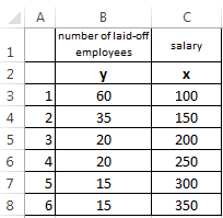
The task. On 6 enterprises was analyzed the average monthly salary and the number of employees who retired. It is necessary to determine the dependence of the number of employees who retired from the average salary.
The linear regression model is as follows:
У = а0 + а1х1 +…+акхк.
Where a – are the regression coefficients, x – the influencing variables, k – the number of factors.
In our example as Y serves the indicator of employees who retired. The influence factor – is the wage (x).
In Excel, there are built-in features with which you can calculate the parameters of the linear regression model. But faster it will make the add-on «analysis package».
Activate the powerful analytical tool:
- Push the button «FILE»-«Options»-«Add-Ins».
- Below the drop-down list in the «Manage:» field is the inscription «Excel Add-Ins» (if it is not, click on the checkbox to the right and select). And click the «Go» button. Hit.
- The list of available add-ins. Select the «Analysis ToolPak» and click OK.
After activating the superstructure will be available on the «DATA» tab.
We direct regression analysis now.
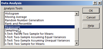
- Open the «Data Analysis» tool menu. Select the «Regression».
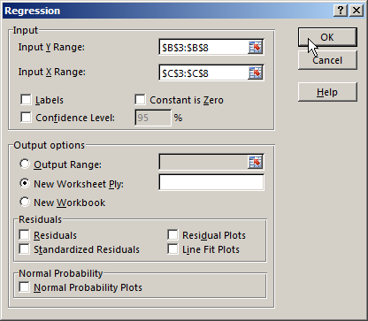
- Open the menu for selecting the input values and output parameters (which display the result). In the fields for the specify range of the input data, which describes the options (Y) and influence the factor (X). The rest can not fill.
- After you click OK, the program will display the calculations on a new page (you can choose the interval to be displayed on the current page or assign to the output to a new book).
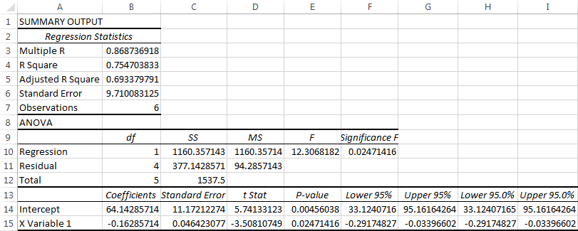
Firstly of all pay attention to the R-squared and the ratios.
R-square – is the coefficient of the determination. In our example – there is 0. 755, or 75. 5%. This means that the model parameters estimated at 75. 5% explains the addiction between the parameters whixh are studied. The higher the coefficient of determination, the better is the model. Good — above 0. 8. Bad — less than 0. 5 (such an analysis can hardly be considered reasonable). In our example – is «not bad».
64. 1428 ratio shows how will be Y, if all the variables in the model will be equal to 0. That is, the value of the analyzed parameter is influenced by other factors, which has not been described in the model.
-0. 16285 ratio shows the weight of the variable X to Y. That is, the average monthly salary in the range of the model affects the number of resignations from the weight -0. 16285 (this is a small effect). The sign «-» indicates to a negative effect: the higher the salary, the less dismissed. That is true.
Correlation analys in Excel
The correlation analysis helps to establish whether there is between the indices in one or two samples of the connection. For example, the time between the time machine and repair costs, equipment costs and operation duration, height and weight of children, etc.
If there is the connection is available, whether the increment of one the increase parameter (positive correlation) or the decreasing (negative) of the other one. The correlation analysis helps to the analyst to determine whether it is possible for the value of one indicator to predict the potential value of the other one.
The correlation coefficient is denoted by r. It ranges from +1 to -1. The classification of correlations for different areas will be different. If the value of the coefficient is 0 linear dependence between samples does not exist.
Consider how with helping Excel tools to find the correlation coefficient.
To find the paired coefficients applied CORREL function.
The task: To determine whether there is the interrelation between the operating time of the lathe and the costing of its maintenance.
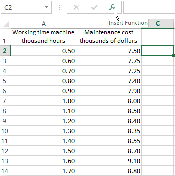
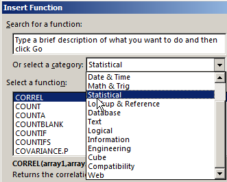
Put the cursor in any cell and click the fx button.
- In «Statistics» category select to the function =CORREL().
- The argument «Array 1» – is the first range of the values — while the machine: A2: A14.
- The argument «Array 2» – is the second range of values — the cost of repairs: B2: B14. Click OK.
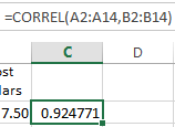
To determine the type of connection, it is necessary to see the absolute number of the coefficient (each a scale has for each field).
Note. For the correlation analysis of several parameters (more 2) it is more convenient to use the «Data Analysis» (add-on «Analysis Package»). In the list you need to choose and mark correlation array. That`s all. These coefficients are appeared in the correlation matrix.
The regression analysis
In practice, these two techniques are often used together.
The example:
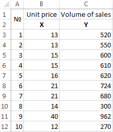
- Build to the correlation field: «INSERT» — «Charts» — «Scatter» (enables to compare pairs). The value range – there are all the numeric dates in the table.
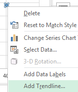
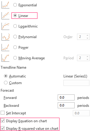
- Click with the left mouse button on any point on the chart. Then right. In the menu, select «Add Trendline».
- Assign the parameters for the line. Type – is «Linear». Below – «Display equation on chart» and «Display R-squared value on chart».
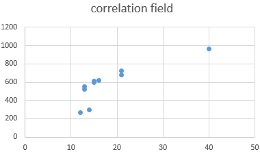
Done:
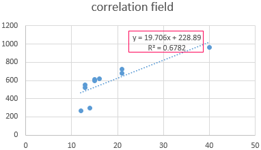
They are now visible and regression analysis dates.
Excel Regression Analysis (Table of Contents)
- Regression Analysis in Excel
- Explanation of Regression Mathematically
- How to Perform Linear Regression in Excel?
- #1 – Regression Tool Using Analysis ToolPak in Excel
- #2 – Regression Analysis Using Scatterplot with Trendline in Excel
What is Regression Analysis in Excel
Linear regression is a statistical technique that examines the linear relationship between a dependent variable and one or more independent variables.
- Dependent Variable (aka response/outcome variable): This is the variable of your interest and wanted to predict based on the Independent variable(s).
- Independent Variable (aka explanatory/predictor variable): Is/are the variable(s) on which response variable is depend. This means these are the variables using which response variables can be predicted.
Linear relationship means the change in an independent variable(s) causes a change in the dependent variable.
There are basically two types of linear relationships as well.
- Positive Linear Relationship: When the independent variable increases, the dependent variable increases too.
- Negative Linear Relationship: When the independent variable increases, the dependent variable decreases.
These were some of the pre-requisites before you actually proceed towards regression analysis in excel.
There are two basic ways to perform linear regression in excel using:
- Regression tool through Analysis ToolPak
- Scatter chart with a trendline
There is actually one more method which is using manual formula’s to calculate linear regression. But why should you go for it when excel does calculations for you?
Therefore, we are going to talk about the two methods discussed above only.
Suppose you have data on the height and weight of 10 individuals. If you plot this information through a chart, let’s see what it gives.
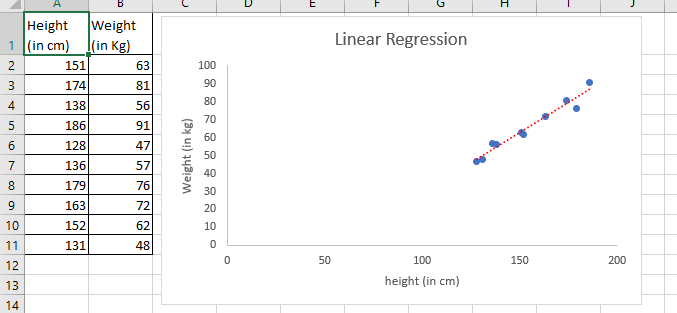
As the above screenshot shows, the linear relationship can be found in Height and Weight through the graph. Don’t get much involved in graphs now; we are anyhow going to dig it deep in the second portion of this article.
Explanation of Regression Mathematically
We have a mathematical expression for linear regression as below:
Y = aX + b + ε
Where,
- Y is a dependent variable or response variable.
- X is an independent variable or predictor.
- a is the slope of the regression line. This represents that when X changes, there is a change in Y by “a” units.
- b is intercepting. It is the value Y takes when the value of X is zero.
- ε is the random error term. It occurs because Y’s predicted value will never be exactly the same as the actual value for a given X. We don’t need to worry about this error term as some software do the calculation of this error term in the backend for you. Excel is one of that software.
In that case, the equation becomes,
Y = aX + b
Which can be represented as:
Weight = a*Height + b
We’ll try to find out the values of this a and b using the methods we have discussed above.
How to Perform Linear Regression in Excel?
The further article explains the basics of regression analysis in excel and shows a few different ways to do linear regression in Excel.
You can download this Regression Analysis Excel Template here – Regression Analysis Excel Template
#1 – Regression Tool Using Analysis ToolPak in Excel
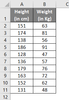
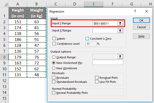
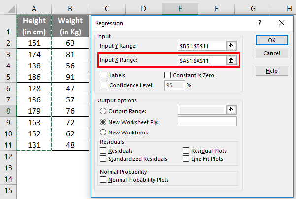
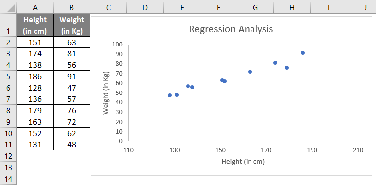
For our example, we’ll try to fit regression for Weight values (which is a dependent variable) with the help of Height values (which is an independent variable).
- In the excel spreadsheet, click on Data Analysis (present under Analysis Group) under Data.
- Search out for Regression. Could you select it and press, ok?
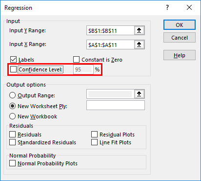
- Use the following inputs under the Regression pane, which opens up.
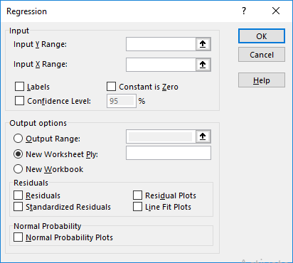
- Input Y Range: Select the cells which contain your dependent variable (in this example, B1:B11)
- Input X Range: Select the cells which contain your independent variable (in this example, A1:A11).
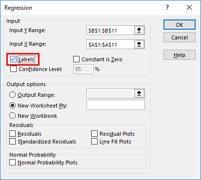
- Check the box named Labels if your data have column names (in this example, we have column names).
- The confidence level is set to 95% by default, which can be changed as per user’s requirements.
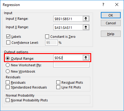
- Under Output options, you can customize where you want to see the regression analysis output in Excel. In this case, we want to see the output on the same sheet. Therefore, the given range is accordingly.
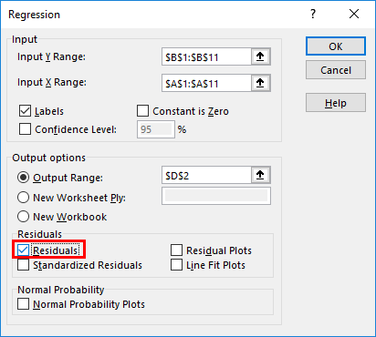
- Under the Residuals option, you have optional inputs like Residuals, Residual Plots, Standardized Residuals, and Line Fit Plots, which you can select as per your need. In this case, check the Residuals checkbox so that we can see the dispersion between predicted and actual values.
- Under the Normal Probability option, you can select Normal Probability Plots, which can help you check the normality of predictors. Click on OK.
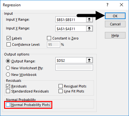
- Excel will compute Regression analysis for you in a fraction of second.
Till here, it was easy and not that logical. However, interpreting this output and make valuable insights from it is a tricky task.
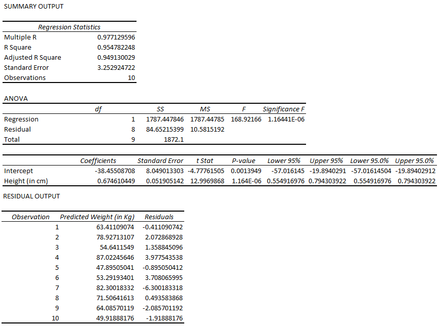
One important part of this entire output is R Square/ Adjusted R Square under the SUMMARY OUTPUT table, which provides information on how well our model is fit. In this case, the R Square value is 0.9547, which interprets that the model has a 95.47% accuracy (good fit). Or in another language, information about the Y variable is explained 95.47% by the X variable.
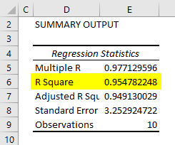
The other important part of the entire output is a table of coefficients. It gives values of coefficients that can be used to build the model for future predictions.
Now our regression equation for prediction becomes:
Weight = 0.6746*Height – 38.45508 (Slope value for Height is 0.6746… and Intercept is -38.45508…)
Did you get what you have defined? You have defined a function in which you now just have to put the value of Height, and you’ll get the Weight value.
#2 – Regression Analysis Using Scatterplot with Trendline in Excel
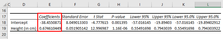
Now, we’ll see how in excel, we can fit a regression equation on a scatterplot itself.
- Select your entire two-columned data (including headers).
- Click on Insert and select Scatter Plot under the graphs section, as shown in the image below.
- See the output graph.
- Now, we need to have the least squared regression line on this graph. To add this line, right-click on any of the graph’s data points and select Add Trendline option.
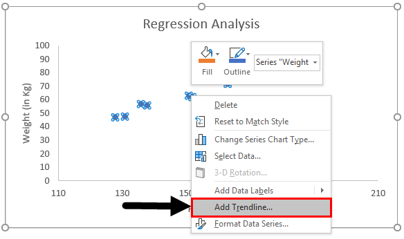
- It will enable you to have a trendline of the least square of regression like below.
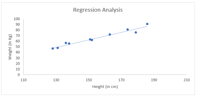
- Under the Format Trendline option, check the box for Display Equation on Chart.
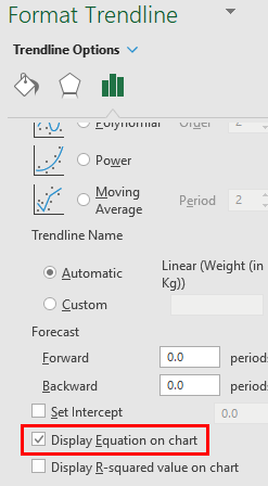
- It enables you to see the equation of the least squared regression line on the graph.
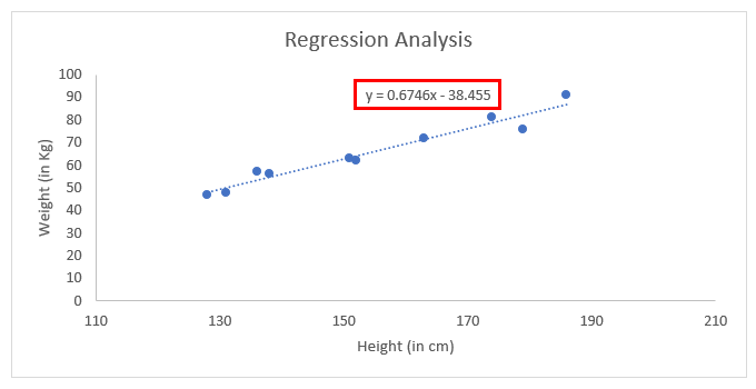
This is the equation using which we can predict the weight values for any given set of Height values.
Things to Remember About Regression Analysis in Excel
- You can change the layout of the trendline under the Format Trendline option in the scatter plot.
- It is always recommended to have a look at residual plots while you are doing regression analysis using Data Analysis ToolPak in Excel. It gives you a better understanding of the spread of the actual Y values and estimated X values.
- Simple Linear Regression in excel does not need ANOVA and Adjusted R Square to check. These features can be considered for Multiple Linear Regression, which is beyond the scope of this article.
Recommended Articles
This has been a guide to Regression Analysis in Excel. Here we discuss how to do Regression Analysis in Excel, along with excel examples and a downloadable excel template. You can also go through our other suggested articles –
- Excel Tool for Data Analysis
- Calculate ANOVA in Excel
- How to find Excel Moving Averages
- Z TEST Examples in Excel