
Logistic regression is a method that we use to fit a regression model when the response variable is binary.
This tutorial explains how to perform logistic regression in Excel.
Example: Logistic Regression in Excel
Use the following steps to perform logistic regression in Excel for a dataset that shows whether or not college basketball players got drafted into the NBA (draft: 0 = no, 1 = yes) based on their average points, rebounds, and assists in the previous season.
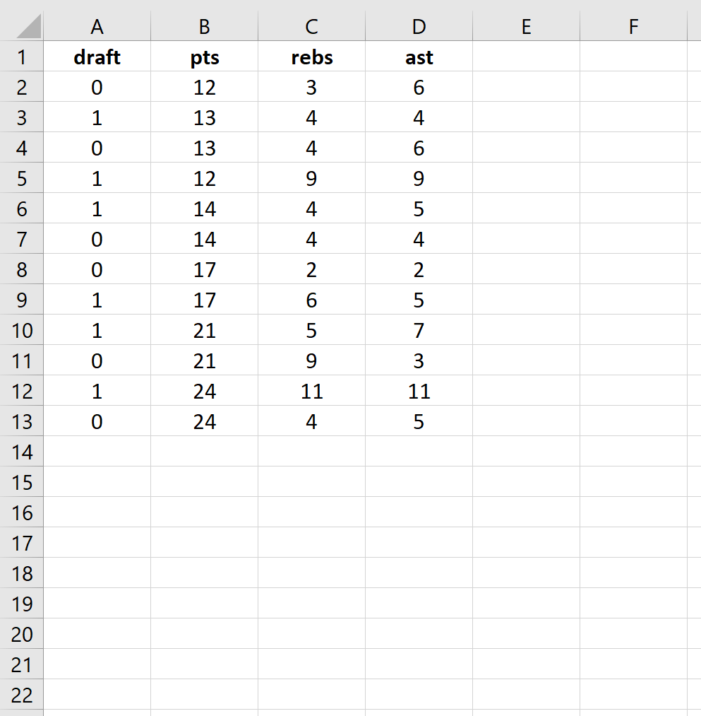
Step 1: Input the data.
First, input the following data:

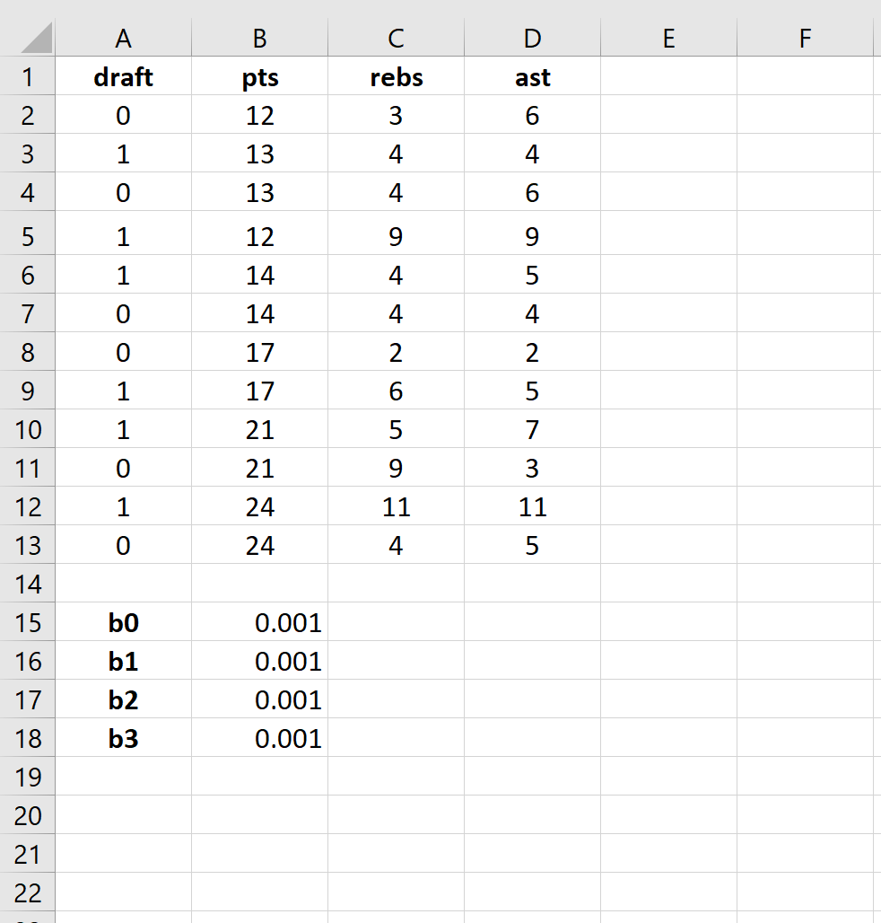
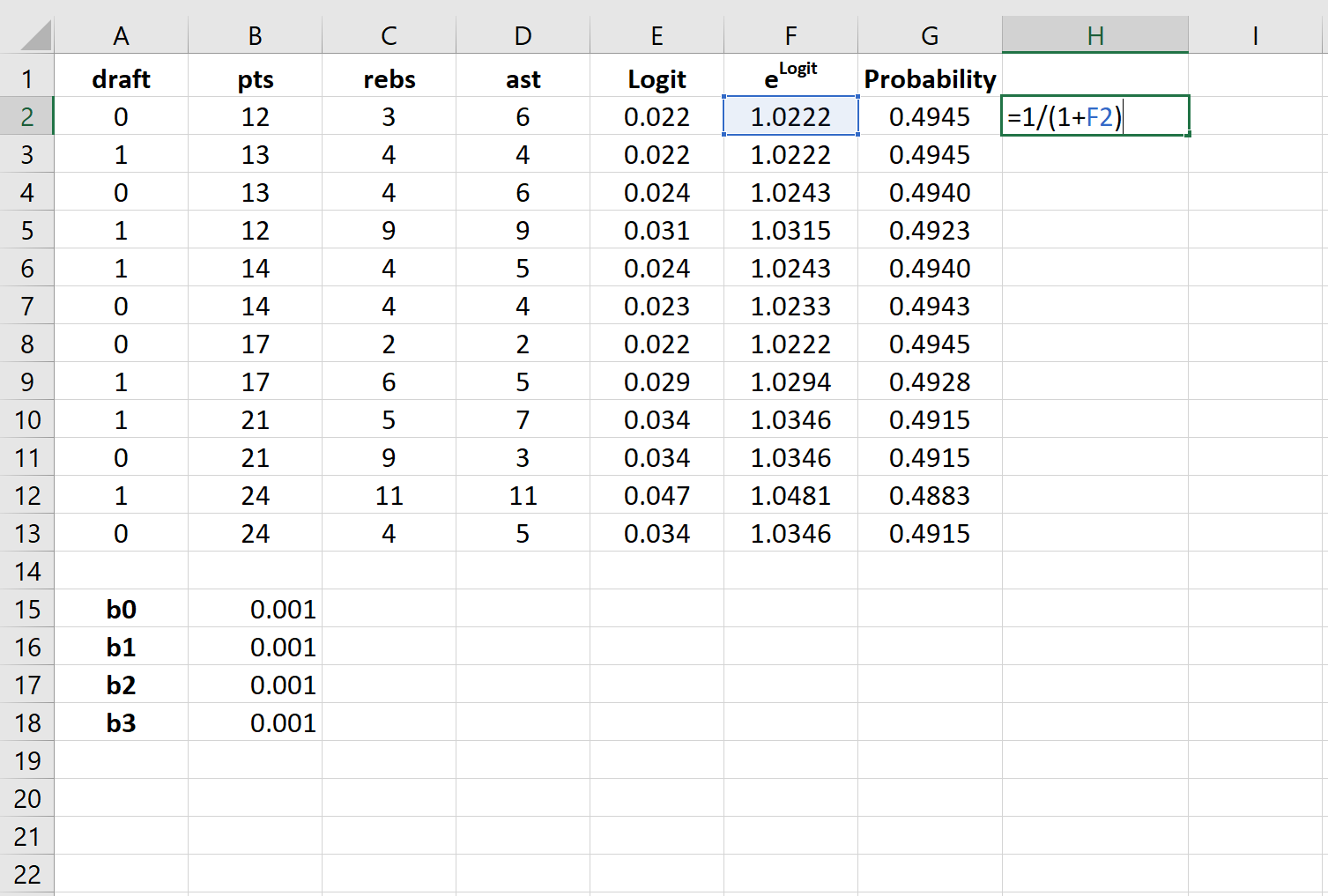
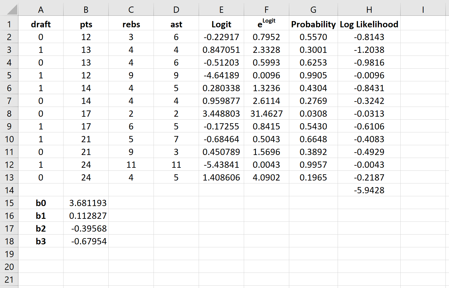
Step 2: Enter cells for regression coefficients.
Since we have three explanatory variables in the model (pts, rebs, ast), we will create cells for three regression coefficients plus one for the intercept in the model. We will set the values for each of these to 0.001, but we will optimize for them later.

Next, we will have to create a few new columns that we will use to optimize for these regression coefficients including the logit, elogit, probability, and log likelihood.
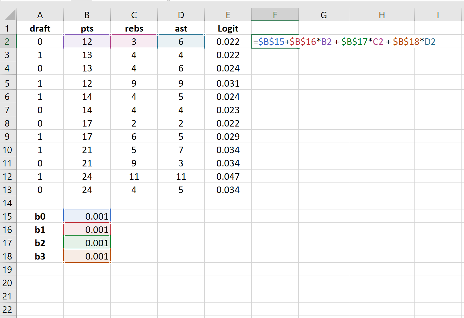
Step 3: Create values for the logit.
Next, we will create the logit column by using the the following formula:

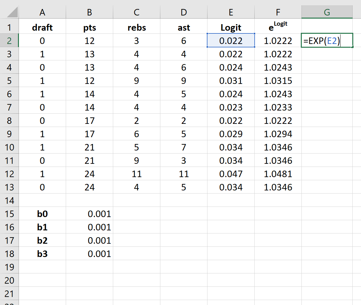
Step 4: Create values for elogit.
Next, we will create values for elogit by using the following formula:

Step 5: Create values for probability.
Next, we will create values for probability by using the following formula:

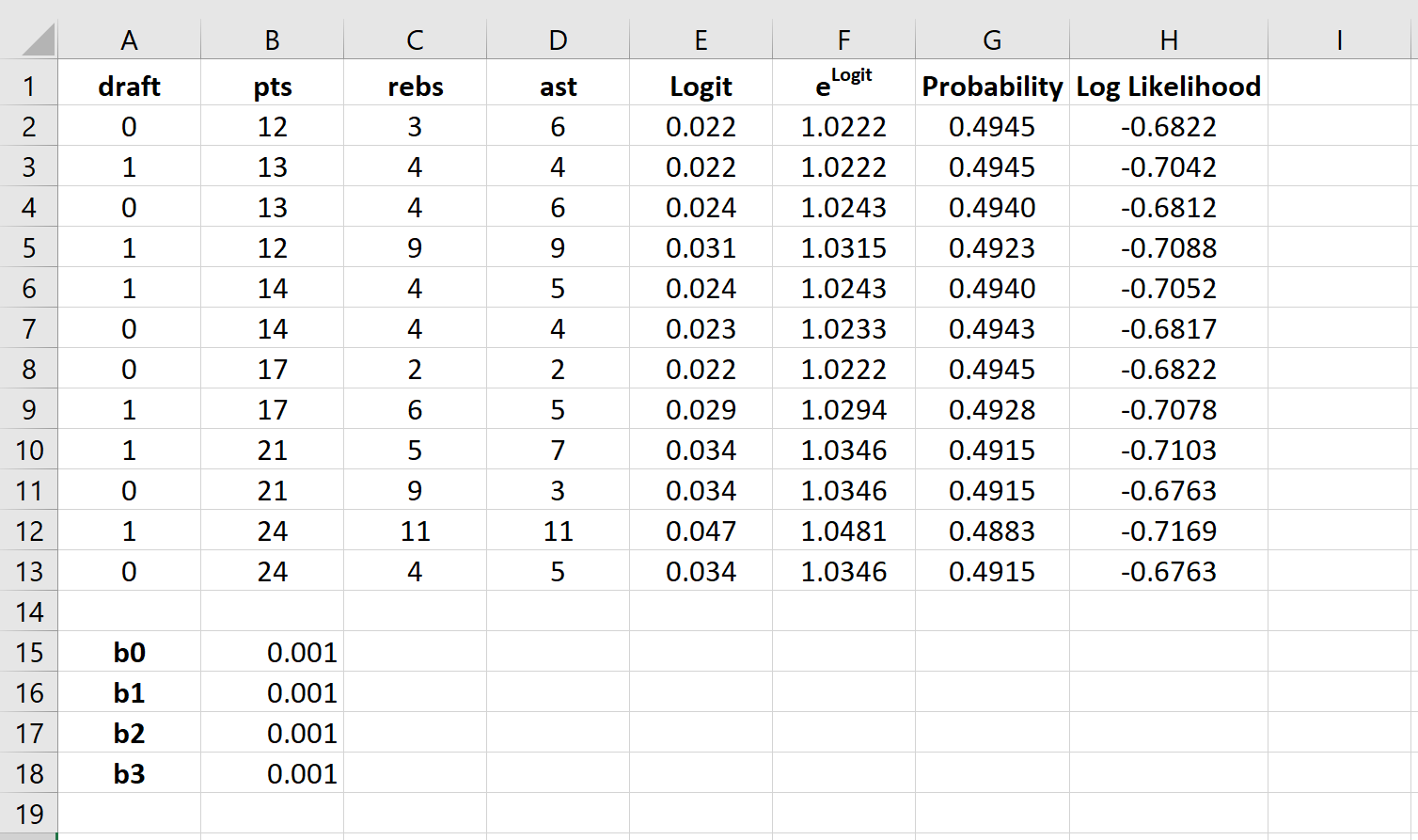
Step 6: Create values for log likelihood.
Next, we will create values for log likelihood by using the following formula:
Log likelihood = LN(Probability)

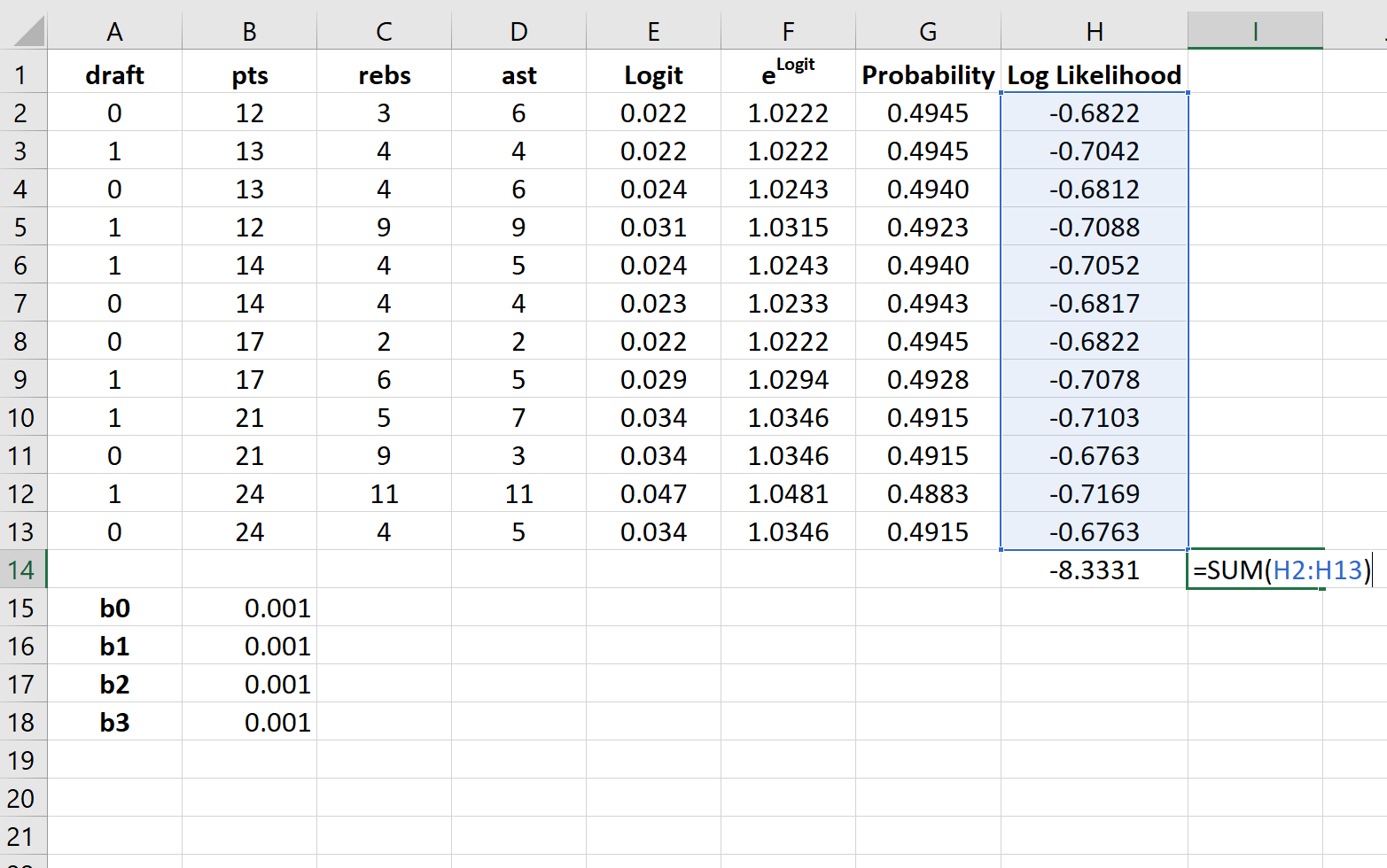
Step 7: Find the sum of the log likelihoods.
Lastly, we will find the sum of the log likelihoods, which is the number we will attempt to maximize to solve for the regression coefficients.

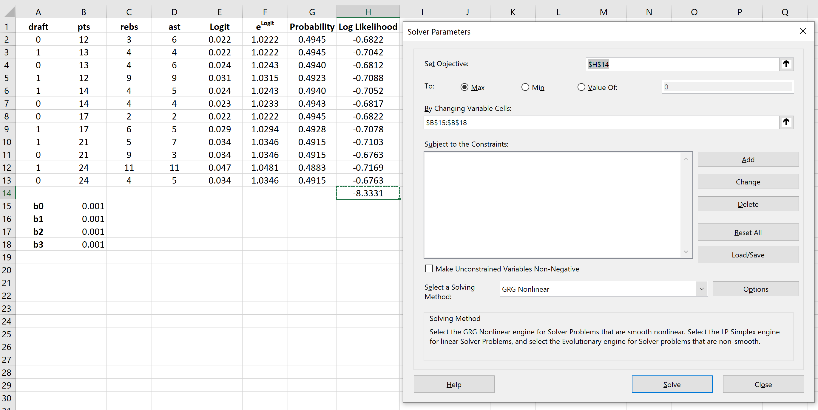
Step 8: Use the Solver to solve for the regression coefficients.
If you haven’t already install the Solver in Excel, use the following steps to do so:
- Click File.
- Click Options.
- Click Add-Ins.
- Click Solver Add-In, then click Go.
- In the new window that pops up, check the box next to Solver Add-In, then click Go.
Once the Solver is installed, go to the Analysis group on the Data tab and click Solver. Enter the following information:
- Set Objective: Choose cell H14 that contains the sum of the log likelihoods.
- By Changing Variable Cells: Choose the cell range B15:B18 that contains the regression coefficients.
- Make Unconstrained Variables Non-Negative: Uncheck this box.
- Select a Solving Method: Choose GRG Nonlinear.
Then click Solve.
The Solver automatically calculates the regression coefficient estimates:

By default, the regression coefficients can be used to find the probability that draft = 0.
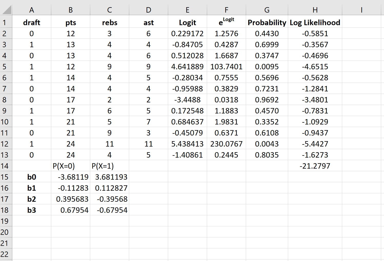
However, typically in logistic regression we’re interested in the probability that the response variable = 1.
So, we can simply reverse the signs on each of the regression coefficients:

Now these regression coefficients can be used to find the probability that draft = 1.
For example, suppose a player averages 14 points per game, 4 rebounds per game, and 5 assists per game. The probability that this player will get drafted into the NBA can be calculated as:
P(draft = 1) = e3.681193 + 0.112827*(14) -0.39568*(4) – 0.67954*(5) / (1+e3.681193 + 0.112827*(14) -0.39568*(4) – 0.67954*(5)) = 0.57.
Since this probability is greater than 0.5, we predict that this player would get drafted into the NBA.
Related: How to Create a ROC Curve in Excel (Step-by-Step)
17 авг. 2022 г.
читать 3 мин
Логистическая регрессия — это метод, который мы используем для подбора регрессионной модели, когда переменная ответа является бинарной.
В этом руководстве объясняется, как выполнить логистическую регрессию в Excel.
Пример: логистическая регрессия в Excel
Используйте следующие шаги, чтобы выполнить логистическую регрессию в Excel для набора данных, который показывает, были ли баскетболисты колледжей выбраны в НБА (драфт: 0 = нет, 1 = да) на основе их среднего количества очков, подборов и передач в предыдущем время года.
Шаг 1: Введите данные.
Сначала введите следующие данные:
Шаг 2: Введите ячейки для коэффициентов регрессии.
Поскольку в модели у нас есть три объясняющие переменные (pts, rebs, ast), мы создадим ячейки для трех коэффициентов регрессии плюс один для точки пересечения в модели. Мы установим значения для каждого из них на 0,001, но мы оптимизируем их позже.
Далее нам нужно будет создать несколько новых столбцов, которые мы будем использовать для оптимизации этих коэффициентов регрессии, включая логит, e логит , вероятность и логарифмическую вероятность.
Шаг 3: Создайте значения для логита.
Далее мы создадим столбец logit, используя следующую формулу:
Шаг 4: Создайте значения для e logit .
Далее мы создадим значения для e logit , используя следующую формулу:
Шаг 5: Создайте значения для вероятности.
Далее мы создадим значения вероятности, используя следующую формулу:
Шаг 6: Создайте значения для логарифмической вероятности.
Далее мы создадим значения для логарифмической вероятности, используя следующую формулу:
Логарифмическая вероятность = LN (вероятность)
Шаг 7: Найдите сумму логарифмических вероятностей.
Наконец, мы найдем сумму логарифмических правдоподобий, то есть число, которое мы попытаемся максимизировать, чтобы найти коэффициенты регрессии.
Шаг 8: Используйте Решатель, чтобы найти коэффициенты регрессии.
Если вы еще не установили Solver в Excel, выполните следующие действия:
- Щелкните Файл .
- Щелкните Параметры .
- Щелкните Надстройки .
- Нажмите Надстройка «Поиск решения» , затем нажмите «Перейти» .
- В новом всплывающем окне установите флажок рядом с Solver Add-In , затем нажмите «Перейти» .
После установки Солвера перейдите в группу Анализ на вкладке Данные и нажмите Солвер.Введите следующую информацию:
- Установите цель: выберите ячейку H14, содержащую сумму логарифмических вероятностей.
- Путем изменения ячеек переменных: выберите диапазон ячеек B15:B18, который содержит коэффициенты регрессии.
- Сделать неограниченные переменные неотрицательными: снимите этот флажок.
- Выберите метод решения: выберите GRG Nonlinear.
Затем нажмите «Решить» .
Решатель автоматически вычисляет оценки коэффициента регрессии:
По умолчанию коэффициенты регрессии можно использовать для определения вероятности того, что осадка = 0. Однако обычно в логистической регрессии нас интересует вероятность того, что переменная отклика = 1. Таким образом, мы можем просто поменять знаки на каждом из коэффициенты регрессии:
Теперь эти коэффициенты регрессии можно использовать для определения вероятности того, что осадка = 1.
Например, предположим, что игрок набирает в среднем 14 очков за игру, 4 подбора за игру и 5 передач за игру. Вероятность того, что этот игрок будет выбран в НБА, можно рассчитать как:
P(draft = 1) = e 3,681193 + 0,112827*(14) -0,39568*(4) – 0,67954*(5) / (1+e 3,681193 + 0,112827*(14) -0,39568*(4) – 0,67954*(5) ) ) = 0,57 .
Поскольку эта вероятность больше 0,5, мы прогнозируем, что этот игрокпопасть в НБА.
Связанный: Как создать кривую ROC в Excel (шаг за шагом)
Содержание
- Как выполнить логистическую регрессию в Excel
- Пример: логистическая регрессия в Excel
- How to Perform Logistic Regression in Excel
- Example: Logistic Regression in Excel
- Do logistic regression excel
Как выполнить логистическую регрессию в Excel

Логистическая регрессия — это метод, который мы используем для подбора регрессионной модели, когда переменная ответа является бинарной.
В этом руководстве объясняется, как выполнить логистическую регрессию в Excel.
Пример: логистическая регрессия в Excel
Используйте следующие шаги, чтобы выполнить логистическую регрессию в Excel для набора данных, который показывает, были ли баскетболисты колледжей выбраны в НБА (драфт: 0 = нет, 1 = да) на основе их среднего количества очков, подборов и передач в предыдущем время года.
Шаг 1: Введите данные.
Сначала введите следующие данные:
Шаг 2: Введите ячейки для коэффициентов регрессии.
Поскольку в модели у нас есть три объясняющие переменные (pts, rebs, ast), мы создадим ячейки для трех коэффициентов регрессии плюс один для точки пересечения в модели. Мы установим значения для каждого из них на 0,001, но мы оптимизируем их позже.
Далее нам нужно будет создать несколько новых столбцов, которые мы будем использовать для оптимизации этих коэффициентов регрессии, включая логит, e логит , вероятность и логарифмическую вероятность.
Шаг 3: Создайте значения для логита.
Далее мы создадим столбец logit, используя следующую формулу:
Шаг 4: Создайте значения для e logit .
Далее мы создадим значения для e logit , используя следующую формулу:
Шаг 5: Создайте значения для вероятности.
Далее мы создадим значения вероятности, используя следующую формулу:
Шаг 6: Создайте значения для логарифмической вероятности.
Далее мы создадим значения для логарифмической вероятности, используя следующую формулу:
Логарифмическая вероятность = LN (вероятность)
Шаг 7: Найдите сумму логарифмических вероятностей.
Наконец, мы найдем сумму логарифмических правдоподобий, то есть число, которое мы попытаемся максимизировать, чтобы найти коэффициенты регрессии.
Шаг 8: Используйте Решатель, чтобы найти коэффициенты регрессии.
Если вы еще не установили Solver в Excel, выполните следующие действия:
- Щелкните Файл .
- Щелкните Параметры .
- Щелкните Надстройки .
- Нажмите Надстройка «Поиск решения» , затем нажмите «Перейти» .
- В новом всплывающем окне установите флажок рядом с Solver Add-In , затем нажмите «Перейти» .
После установки Солвера перейдите в группу Анализ на вкладке Данные и нажмите Солвер.Введите следующую информацию:
- Установите цель: выберите ячейку H14, содержащую сумму логарифмических вероятностей.
- Путем изменения ячеек переменных: выберите диапазон ячеек B15:B18, который содержит коэффициенты регрессии.
- Сделать неограниченные переменные неотрицательными: снимите этот флажок.
- Выберите метод решения: выберите GRG Nonlinear.
Затем нажмите «Решить» .
Решатель автоматически вычисляет оценки коэффициента регрессии:
По умолчанию коэффициенты регрессии можно использовать для определения вероятности того, что осадка = 0. Однако обычно в логистической регрессии нас интересует вероятность того, что переменная отклика = 1. Таким образом, мы можем просто поменять знаки на каждом из коэффициенты регрессии:
Теперь эти коэффициенты регрессии можно использовать для определения вероятности того, что осадка = 1.
Например, предположим, что игрок набирает в среднем 14 очков за игру, 4 подбора за игру и 5 передач за игру. Вероятность того, что этот игрок будет выбран в НБА, можно рассчитать как:
P(draft = 1) = e 3,681193 + 0,112827*(14) -0,39568*(4) – 0,67954*(5) / (1+e 3,681193 + 0,112827*(14) -0,39568*(4) – 0,67954*(5) ) ) = 0,57 .
Поскольку эта вероятность больше 0,5, мы прогнозируем, что этот игрокпопасть в НБА.
Источник
How to Perform Logistic Regression in Excel
Logistic regression is a method that we use to fit a regression model when the response variable is binary.
This tutorial explains how to perform logistic regression in Excel.
Example: Logistic Regression in Excel
Use the following steps to perform logistic regression in Excel for a dataset that shows whether or not college basketball players got drafted into the NBA (draft: 0 = no, 1 = yes) based on their average points, rebounds, and assists in the previous season.
Step 1: Input the data.
First, input the following data:
Step 2: Enter cells for regression coefficients.
Since we have three explanatory variables in the model (pts, rebs, ast), we will create cells for three regression coefficients plus one for the intercept in the model. We will set the values for each of these to 0.001, but we will optimize for them later.
Next, we will have to create a few new columns that we will use to optimize for these regression coefficients including the logit, e logit , probability, and log likelihood.
Step 3: Create values for the logit.
Next, we will create the logit column by using the the following formula:
Step 4: Create values for e logit .
Next, we will create values for e logit by using the following formula:
Step 5: Create values for probability.
Next, we will create values for probability by using the following formula:
Step 6: Create values for log likelihood.
Next, we will create values for log likelihood by using the following formula:
Log likelihood = LN(Probability)
Step 7: Find the sum of the log likelihoods.
Lastly, we will find the sum of the log likelihoods, which is the number we will attempt to maximize to solve for the regression coefficients.
Step 8: Use the Solver to solve for the regression coefficients.
If you haven’t already install the Solver in Excel, use the following steps to do so:
- Click File.
- Click Options.
- Click Add-Ins.
- Click Solver Add-In, then click Go.
- In the new window that pops up, check the box next to Solver Add-In, then click Go.
Once the Solver is installed, go to the Analysis group on the Data tab and click Solver. Enter the following information:
- Set Objective: Choose cell H14 that contains the sum of the log likelihoods.
- By Changing Variable Cells: Choose the cell range B15:B18 that contains the regression coefficients.
- Make Unconstrained Variables Non-Negative: Uncheck this box.
- Select a Solving Method: Choose GRG Nonlinear.
Then click Solve.
The Solver automatically calculates the regression coefficient estimates:
By default, the regression coefficients can be used to find the probability that draft = 0.
However, typically in logistic regression we’re interested in the probability that the response variable = 1.
So, we can simply reverse the signs on each of the regression coefficients:
Now these regression coefficients can be used to find the probability that draft = 1.
For example, suppose a player averages 14 points per game, 4 rebounds per game, and 5 assists per game. The probability that this player will get drafted into the NBA can be calculated as:
P(draft = 1) = e 3.681193 + 0.112827*(14) -0.39568*(4) – 0.67954*(5) / (1+e 3.681193 + 0.112827*(14) -0.39568*(4) – 0.67954*(5) ) = 0.57.
Since this probability is greater than 0.5, we predict that this player would get drafted into the NBA.
Источник
Do logistic regression excel
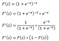
A logit model is a type of a binary choice model. We use a logistic equation to assign a probability to an event. We define a logistic cumulative density function as:

which is equivalent to


Another property of the logistic function is that:

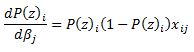
The first derivative of the logistic function, which we will need when deriving the coefficients of our model, with respect to z is:

In a logistic regression model we set up the equation below:

In this set up using ordinary least squares to estimate the beta coefficients is impossible so we must rely on maximum likelihood method.
Under the assumption that each observation of the dependent variable is random and independent we can derive a likelihood function. The likelihood that we observe our existing sample under the assumption of independence is simply the product of the probability of each observation.
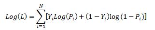
Our likelihood function is:

Where Y is either 0 or 1. We can see that when Y =1 then we have P and when Y=0 we have (1-P)
The aim of the maximum likelihood method is to derive the coefficients of the model that maximize the likelihood function. It is much easier to work with the log of the likelihood function.

From calculus we know that a functions maximum is at a point where its first derivative is equal to zero. Therefore our approach is to take the derivative of the log likelihood function with respect to each beta and derive the value of betas for which the first derivative is equal to zero. This cannot be done analytically unfortunately so we must resolve to using a numerical method. Fortunately for us the log likelihood function has nice properties that allows us to use Newton’s method to achieve this.
Newton’s method is easiest to understand in a univariate set up. It is a numerical method for finding a root of a function by successively making better approximations to the root based on the functions gradient (first derivative).
As a quick example we know that we can approximate a function using first order Taylor series approximation.

where Xc is the current estimate of the root. By setting the function to zero we get

This means that in each step of the algorithm we can improve on an initial guess for x using above rule. Same principles apply to a multivariate system of equations:

Here x is a vector of x values and J is the Jacobian matrix of first derivatives evaluated at vector xc and F is the value of the function evaluated at using latest estimates of x.
Coming back to our logistic regression problem what we are trying to do is to figure out a combination of beta parameters for which our log likelihood function is at a maximum which is equivalent to deriving the set of coefficients where the first derivatives of the likelihood function are all equal to zero. We will do this by using Newton’s numerical method. In the notation from above F is the collection of our log likelihood function’s derivatives with respect to each beta and J is the Hessian matrix of second order partial derivatives of the likelihood function with respect to each beta.
It is a little tedious but necessary to work out these derivatives analytically so we can feed them into our spreadsheet.
Lets restate the log likelihood function once more:

And lets remember that in our case Pi is modeled as:

We will list all the steps in the calculations for those who wish to double check the work
First lets calculate

and via chain rule


and via chain rule

Now we can work through the derivative of our likelihood function.

The derivative of Y with respect to beta (highlighted in red) is equal to zero so we are left with:

Now we can substitute our calculated derivatives:

Values in red cancel out and we are left with:

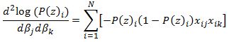
Now we need to calculate the Hessian matrix. Remembering that:


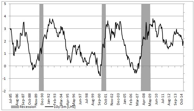
To show an example of how to implement this in excel we will attempt to model the probability of a recession in US (as defined by NBER) with a 3 month lead time. In our set up Y = 1 if US experiences a recession in 3months time and 0 otherwise. Our explanatory variable will be the 10yr3mth treasury curve spread. The yield curve is widely considered to be a leading indicator for economic slowdowns and curve inversion is often considered a sign of a recession.
In the chart below we highlight US recessions in grey while the black line is the yield curve.
The model we are trying to estimate is:

In a spreadsheet we load data on historical recessions in column C and our dependent variable in column D which refers to column C but 3 months ahead. In column E we input 1 which will be our intercept. Column F has historical values for the yield curve. In column G we calculate the probability with the above formula. Our initial guess for betas is zero which we have entered in cell C2 and C3.

In column H we calculate the log likelihood function for each observation. we sum all the values in cell H5. Therefore H5 contains the value of the below formula while each row has a value for each i in the brackets.

Column I calculates the derivative of the likelihood function for each observation with respect to the intercept. Column J calculates the derivative of the likelihood function for each observation with respect to the second beta. The sum of the totals for each column are in cells I2 and I3.

Now we need to calculate the second order derivatives of the likelihood function with respect to each beta. We need 4 in total but remembering that (hessian matrix is symmetric) we only need to calculate 3 columns.

Column K through M calculates the partial derivatives for each row and the sums are reported in a matrix in range J2:K3

Now we finally need to calculate the incremental adjustment to our beta estimates as dictated by the Newton algorithm.

We can use Excel’s functions MINVERSE to calculate the inverse of the Hessian matrix and MMULT function to multiply by our Jacobian matrix. Inputting =MMULT(MINVERSE(J2:K3),I2:I3) in range H2:H3 and pressing Ctrl+Shift+Enter since these are array functions we get the marginal adjustment needed.
Finally in G2 we calculate the adjusted intercept beta by subtracting H2 from C2. We do the same for the second beta.

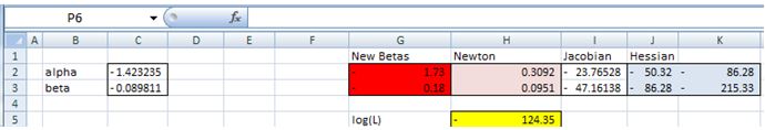
All the calculations shown so far constitute just one iteration of the Newton algorithm. The results so far look like below:

we can copy and paste as values range G2:G3 to C2:C3 to calculate the second iteration of the algorithm

Notice that the log likelihood function has increased. We now have our new estimates in G2:G3. We can copy and paste as values into C2:C3 again. And we should repeat this until the Jacobian matrix is showing zeroes. Once both entries in I2:I3 are zero our log likelihood function is at a maximum.
The algorithm has converged after only 6 iterations and we get below estimates for betas

Overall the model does a poor job of forecasting recessions. The red line shows the probabilities.

In a follow up post we will show how to implement logistic regression in VBA. We will also introduce statistical methods to validate the model and to check for statistical significance of the estimated parameters.
A final note, in this post we wanted to provide a thorough explanation of the logistic regression model and the empirical example we have chosen is too simplistic to be used in practice. However using this approach to model recession probabilities can be very fruitful. Below is an example of a six factor model using the same techniques that forecasts historical recession episodes very well.
Источник
Objective
We now show how to find the coefficients for the logistic regression model using Excel’s Solver capability (see also Goal Seeking and Solver). We start with Example 1 from Basic Concepts of Logistic Regression.
Example
Example 1 (Example 1 from Basic Concepts of Logistic Regression continued): From Definition 1 of Basic Concepts of Logistic Regression, the predicted values pi for the probability of survival for each interval i is given by the following formula where xi represents the number of rems for interval i.
![]()
The log-likelihood statistic as defined in Definition 5 of Basic Concepts of Logistic Regression is given by

where yi is the observed value for survival in the ith interval (i.e. yi = the fraction of subjects in the ith interval that survived). Since we are aggregating the sample elements into intervals, we use the modified version of the formula, namely

where yi is the observed value of survival in the ith of r intervals and
 Initializing Solver
 Initializing Solver
We capture this information in the worksheet in Figure 1 (based on the data in Figure 2 of Basic Concepts of Logistic Regression).

Figure 1 – LL based on an initial guess of coefficients
Column I contains the rem values for each interval (copy of columns A and E). Column J contains the observed probability of survival for each interval (copy of column F). Also, column K contains the values of each pi. E.g. cell K4 contains the formula =1/(1+EXP(-O5–O6*I4)) and initially has a value of 0.5 based on the initial guess of the coefficients a and b given in cells O5 and O6 (which we arbitrarily set to zero). Cell L14 contains the value of LL using the formula =SUM(L4:L13); where L4 contains the formula =(B4+C4)*(J4*LN(K4)+(1-J4)*LN(1-K4)), and similarly for the other cells in column L.
Fill in Solver dialog box
We now use Excel’s Solver tool by selecting Data > Analysis|Solver and filling in the dialog box that appears as described in Figure 2 (see Goal Seeking and Solver for more details).

Figure 2 – Excel Solver dialog box
Our objective is to maximize the value of LL (in cell L14) by changing the coefficients (in cells O5 and O6). It is important, however, to make sure that the Make Unconstrained Variables Non-Negative checkbox is not checked. When we click on the Solve button we get a message that Solver has successfully found a solution, i.e. it has found values for a and b which maximize LL.
Output from Solver
We elect to keep the solution found and Solver automatically updates the worksheet from Figure 1 based on the values it found for a and b. The resulting worksheet is shown in Figure 3.

Figure 3 – Revised version of Figure 1 based on Solver’s solution
We see that a = 4.476711 and b = -0.00721. Thus the logistics regression model is given by the formula
![]()
For example, the predicted probability of survival when exposed to 380 rems of radiation is given by
![]()
Note that
![]()
Thus, the odds that a person exposed to 180 rems survives is 15.5% greater than a person exposed to 200 rems.
Data Analysis Tool
Real Statistics Data Analysis Tool: The Real Statistics Resource Pack provides the Logistic and Probit Regression data analysis tool. This tool takes as input a range that lists the sample data followed by the number of occurrences of success and failure. For Example 1 this is the data in range A3:C13 of Figure 1. For this example, there is only one independent variable (number of rems). If additional independent variables are used then the input will contain additional columns, one for each independent variable.
We now show how to use this tool to create a spreadsheet similar to the one in Figure 3. First, press Ctrl-m to bring up the menu of Real Statistics data analysis tools. Next, choose the Binary Logistic and Probit Regression option from the Reg tab, and press the OK button. (The sequence of steps is slightly different if using the original user interface). This brings up the dialog box shown in Figure 4.
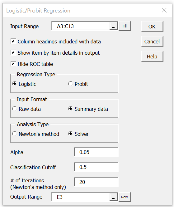
Figure 4 – Dialog Box for Logistic Regression data analysis tool
Now select A3:C13 as the Input Range (see Figure 5). Since this data is in summary form with column headings, select the Summary data option for the Input Format and check Column headings included with data.
Next, select the Solver as the Analysis Type and keep the default Alpha and Classification Cutoff values of .05 and .5 respectively. Since we have selected the Solver option, we also need to select the Show item by item details in output option.
Observations
This tool takes as input a range that lists the sample data followed by the number of occurrences of success and failure (this is considered to be the summary form). E.g. for Example 1 this is the data in range A3:C13 of Figure 1 (repeated in Figure 5 in the same cells). For this problem, there was only one independent variable (number of rems). If additional independent variables are used then the input will contain additional columns, one for each independent variable.
Output from data analysis tool
Finally, press the OK button to obtain the output displayed in Figure 5.
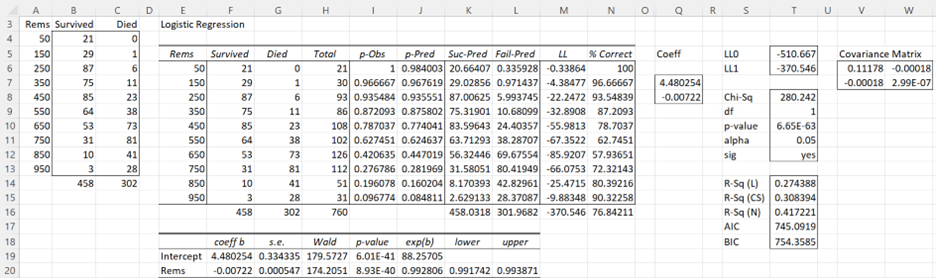
Figure 5 – Output from Logistic Regression tool
Note that the regression coefficients in Q7:Q8 are the same as those we obtained previously in Figure 3. The output from the Logistic Regression data analysis tool also contains many fields which will be explained elsewhere.
Note that the data analysis tool initially sets the coefficients (range Q7:Q8) to zero and so LL (cell M16) is calculated to be -526.792 (exactly as in Figure 1). As described in Figure 2, the data analysis tool then uses Solver to find the logistic regression coefficients shown in Figure 5 (and calculates other interesting values as well).
Examples Workbook
Click here to download the Excel workbook with the examples described on this webpage.
References
Howell, D. C. (2010) Statistical methods for psychology (7th ed.). Wadsworth, Cengage Learning.
https://labs.la.utexas.edu/gilden/files/2016/05/Statistics-Text.pdf
Christensen, R. (2013) Logistic regression: predicting counts.
http://stat.unm.edu/~fletcher/SUPER/chap21.pdf
Wikipedia (2012) Logistic regression
https://en.wikipedia.org/wiki/Logistic_regression
Agresti, A. (2013) Categorical data analysis, 3rd Ed. Wiley.
https://mybiostats.files.wordpress.com/2015/03/3rd-ed-alan_agresti_categorical_data_analysis.pdf
A logit model is a type of a binary choice model. We use a logistic equation to assign a probability to an event. We define a logistic cumulative density function as:

which is equivalent to


Another property of the logistic function is that:

The first derivative of the logistic function, which we will need when deriving the coefficients of our model, with respect to z is:
In a logistic regression model we set up the equation below:

In this set up using ordinary least squares to estimate the beta coefficients is impossible so we must rely on maximum likelihood method.
Under the assumption that each observation of the dependent variable is random and independent we can derive a likelihood function. The likelihood that we observe our existing sample under the assumption of independence is simply the product of the probability of each observation.
Our likelihood function is:

Where Y is either 0 or 1. We can see that when Y =1 then we have P and when Y=0 we have (1-P)
The aim of the maximum likelihood method is to derive the coefficients of the model that maximize the likelihood function. It is much easier to work with the log of the likelihood function.
From calculus we know that a functions maximum is at a point where its first derivative is equal to zero. Therefore our approach is to take the derivative of the log likelihood function with respect to each beta and derive the value of betas for which the first derivative is equal to zero. This cannot be done analytically unfortunately so we must resolve to using a numerical method. Fortunately for us the log likelihood function has nice properties that allows us to use Newton’s method to achieve this.
Newton’s method is easiest to understand in a univariate set up. It is a numerical method for finding a root of a function by successively making better approximations to the root based on the functions gradient (first derivative).
As a quick example we know that we can approximate a function using first order Taylor series approximation.

where Xc is the current estimate of the root. By setting the function to zero we get

This means that in each step of the algorithm we can improve on an initial guess for x using above rule. Same principles apply to a multivariate system of equations:

Here x is a vector of x values and J is the Jacobian matrix of first derivatives evaluated at vector xc and F is the value of the function evaluated at using latest estimates of x.
Coming back to our logistic regression problem what we are trying to do is to figure out a combination of beta parameters for which our log likelihood function is at a maximum which is equivalent to deriving the set of coefficients where the first derivatives of the likelihood function are all equal to zero. We will do this by using Newton’s numerical method. In the notation from above F is the collection of our log likelihood function’s derivatives with respect to each beta and J is the Hessian matrix of second order partial derivatives of the likelihood function with respect to each beta.
It is a little tedious but necessary to work out these derivatives analytically so we can feed them into our spreadsheet.
Lets restate the log likelihood function once more:
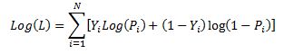
And lets remember that in our case Pi is modeled as:

We will list all the steps in the calculations for those who wish to double check the work
First lets calculate

and via chain rule

Therefore

Also,

and via chain rule

Now we can work through the derivative of our likelihood function.

The derivative of Y with respect to beta (highlighted in red) is equal to zero so we are left with:

Now we can substitute our calculated derivatives:

Values in red cancel out and we are left with:

Now we need to calculate the Hessian matrix. Remembering that:
we have:
To show an example of how to implement this in excel we will attempt to model the probability of a recession in US (as defined by NBER) with a 3 month lead time. In our set up Y = 1 if US experiences a recession in 3months time and 0 otherwise. Our explanatory variable will be the 10yr3mth treasury curve spread. The yield curve is widely considered to be a leading indicator for economic slowdowns and curve inversion is often considered a sign of a recession.
In the chart below we highlight US recessions in grey while the black line is the yield curve.

The model we are trying to estimate is:
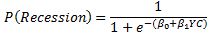
In a spreadsheet we load data on historical recessions in column C and our dependent variable in column D which refers to column C but 3 months ahead. In column E we input 1 which will be our intercept. Column F has historical values for the yield curve. In column G we calculate the probability with the above formula. Our initial guess for betas is zero which we have entered in cell C2 and C3.

In column H we calculate the log likelihood function for each observation. we sum all the values in cell H5. Therefore H5 contains the value of the below formula while each row has a value for each i in the brackets.

Column I calculates the derivative of the likelihood function for each observation with respect to the intercept. Column J calculates the derivative of the likelihood function for each observation with respect to the second beta. The sum of the totals for each column are in cells I2 and I3.

Now we need to calculate the second order derivatives of the likelihood function with respect to each beta. We need 4 in total but remembering that (hessian matrix is symmetric) we only need to calculate 3 columns.

Column K through M calculates the partial derivatives for each row and the sums are reported in a matrix in range J2:K3

Now we finally need to calculate the incremental adjustment to our beta estimates as dictated by the Newton algorithm.
Remember:

We can use Excel’s functions MINVERSE to calculate the inverse of the Hessian matrix and MMULT function to multiply by our Jacobian matrix. Inputting =MMULT(MINVERSE(J2:K3),I2:I3) in range H2:H3 and pressing Ctrl+Shift+Enter since these are array functions we get the marginal adjustment needed.
Finally in G2 we calculate the adjusted intercept beta by subtracting H2 from C2. We do the same for the second beta.

All the calculations shown so far constitute just one iteration of the Newton algorithm. The results so far look like below:

we can copy and paste as values range G2:G3 to C2:C3 to calculate the second iteration of the algorithm
Notice that the log likelihood function has increased. We now have our new estimates in G2:G3. We can copy and paste as values into C2:C3 again. And we should repeat this until the Jacobian matrix is showing zeroes. Once both entries in I2:I3 are zero our log likelihood function is at a maximum.
The algorithm has converged after only 6 iterations and we get below estimates for betas

Overall the model does a poor job of forecasting recessions. The red line shows the probabilities.

In a follow up post we will show how to implement logistic regression in VBA. We will also introduce statistical methods to validate the model and to check for statistical significance of the estimated parameters.
A final note, in this post we wanted to provide a thorough explanation of the logistic regression model and the empirical example we have chosen is too simplistic to be used in practice. However using this approach to model recession probabilities can be very fruitful. Below is an example of a six factor model using the same techniques that forecasts historical recession episodes very well.

This tutorial will help you set up and interpret a Logistic Regression in Excel using the XLSTAT software.
Not sure this is the modeling feature you are looking for? Check out this guide.
Principles of the logistic regression
Logistic regression, and associated methods such as Probit analysis, are very useful when we want to understand or predict the effect of one or more variables on a binary response variable, i.e. one that can only take two values 0/1 or Yes/No for example.
A logistic regression will be very useful to model the effect of doses of medication in medicine, doses of chemical components in agriculture, or to evaluate the propensity of customers to answer a mailing, or to measure the risk of a customer not paying back a loan in a bank.
With XLSTAT, it is possible to run logistic regression either directly on raw data (the answer is 0 or 1) or on aggregated data (the answer is a sum of successes — of 1 for example — and in this case the number of repetitions must also be available).
Logistic regression models the probability of an event occurring given the values of a set of quantitative and/or qualitative descriptive variables.
Data set for running a binary logit model
The example we consider below is a marketing scenario in which we try to predict the probability that a customer will renew his subscription to an online information service.
The data correspond to a sample of 60 readers, with the age category, the average number of page views per week over the last 10 weeks, and the number of page views during the last week. These readers were asked to renew their subscription which is due to expire in two weeks.
The goal is to understand why some have re-subscribed while others have not.
Goal of this tutorial on logistic regression
The goal is to use binary logistic regression to understand the results obtained from the study and then to apply the model to the entire population in order to identify people who might not renew their subscription.
With this information, the marketer can offer them a promotion or additional services to stimulate their interest in the offer.
Setting up a binary logit model
To activate the Binary Logit Model dialog box, start XLSTAT, then select the XLSTAT / Modeling data / Logistic regression.
Once you have clicked on the button, the dialog box appears. Select the data on the Excel sheet.
The Response data refers to the column in which the binary or quantitative variable is found (resulting then from a sum of binaries — in this case the «Weights» column must be selected next).
In our case there are three explanatory variables, one qualitative — the age class — and two quantitative corresponding to the counts of page views.
Since we have selected the labels of the variables, we must select the option Variable labels.

Once you have clicked on the OK button, the calculations are performed and the results displayed.
Interpret the results of a binary logit model
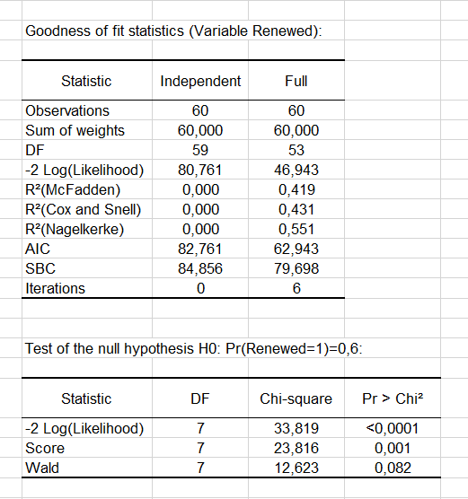
The goodness-of-fit statistics table gives several indicators of the quality of the model (or goodness of fit). These results are equivalent to the R² in the linear regression and to the ANOVA table. The most important value is the Chi² associated with the Log ratio (L.R.). It is the equivalent of Fisher’s F-test of the linear model: we try to evaluate if the variables provide a significant amount of information to explain the variability of the response variable. In our case, as the probability is lower than 0.0001, we can conclude that the variables bring a significant amount of information.
Next, the Type II analysis table gives the first details about the model. It is useful for evaluating the contribution of the variables to the explanation of the response variable.

From the probability associated with the Chi-square tests, we can see that the variable that most influences the renewal is the number of pages viewed the previous week (p = 0.012).
As the Age variable is qualitative (because it is divided into groups), we can determine whether each modality influences the renewal decision. It appears that the group of “40-49” age has a significant negative impact (-2.983). Marketing and editorial managers can investigate this further to understand why. The other age groups do not have any significant effect.

Next, you can view the Predictions and Residuals table. We can see that for the 7th observation, the reader claims not to be interesting in renewing his subscription whereas the model predicts a renewal of the subscription. Indeed we can see that the probability of renewing is estimated at 0.757 while the probability of not renewing is estimated at 0.243.
The column Significant change indicates that the change in value between the predicted modality and the observed one. The second column Significant indicates if the probability of the predicted modality is significantly different than the ones of the other modalities. In the case of the 7th observation, we can see that the change is significant and the probability of renewing (0.757) is higher than that of not renewing (0.243).
Note that these two columns appear if the Significance analysis option has been checked in the «Outputs» tab of the dialog box.

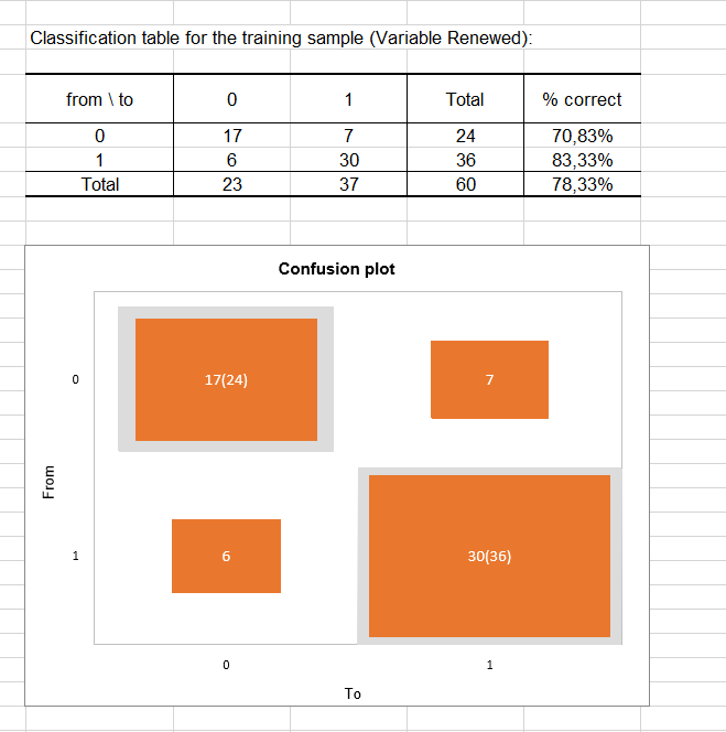
The classification table for the training sample (sometimes called the confusion matrix) is then displayed in the report. This table shows the percentage of observations that were well classified for each modality (true positives and true negatives). For example, we can see that the observations of modality 0 (no renewal) were well classified at 70.83% while the observations of modality 1 (renewal) were well classified at 83.33%.
The confusion plot allows to visualize this table in a synthetic way. The grey squares on the diagonal represent the observed numbers for each modality. The orange squares represent the predicted numbers for each modality. Thus, we can see that the surfaces of the squares almost completely overlap for the two modalities (17 well predicted observations out of 24 observed observations for modality 0 and 30 well predicted observations out of 36 observed observations for modality 1).
Finally, the last two tables take into account the uncertainty. Most the predictions made for modality 0 can be considered as uncertain (95.83%), while for modality 1 the predictions are much less uncertain with a percentage of uncertainty being at estimated at 33.33%.
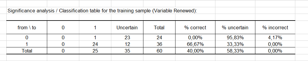
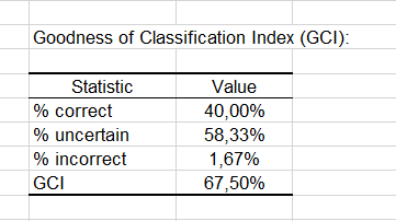
The GCI table shows that 40% of the observations were well classified (true positives), 58.33% had an uncertain classification and only 1.67% were incorrectly classified (false positives and false negatives cumulated). The GCI (Goodness of Classification Index) is 67.50%, which means that the predictive quality of this classification model is good.
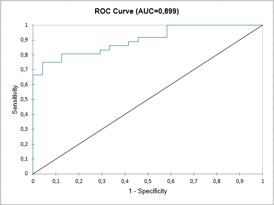
At the end of the XLSTAT output sheet, the ROC curve is displayed. It is used to visualize the performance of a model, and to compare it with that of other models.
The area under the curve (or AUC ) is a synthetic index calculated for ROC curves. The AUC corresponds to the probability such that a positive event has a higher probability given to it by the model than a negative event. For an ideal model, AUC=1 and for a random model, AUC = 0.5. A model is usually considered good when the AUC value is greater than 0.7. A well-discriminating model must have an AUC of between 0.87 and 0.9. A model with an AUC greater than 0.9 is excellent.
Was this article useful?
- Yes
- No

Learn Logistic Regression using Excel — Machine Learning Algorithm
Logistic Regression using Excel: A Beginner’s guide to learn the most well known and well-understood algorithm in statistics and machine learning. In this post, you will discover everything Logistic Regression using Excel algorithm, how it works using Excel, application and it’s pros and cons.
Quick facts about Logistic Regression
Logistic Regression using Excel is a statistical classification technique that can be used in market research
Logistic Regression algorithm is similar to regular linear regression.
The factual part is, Logistic regression data sets in Excel actually produces an estimate of the probability of a certain event occurring
Scenario:
– Logistic Regression Excel is an add-in also, a multidimensional feature space (features can be categorical or continuous)
– An outcome is discrete, not continuous if you know how Logistic Regression in Excel Works.
– Logistic Regression Software seems plausible that a linear decision boundary (hyperplane) will give good predictive accuracy
Watch a video on Logistic Regression
What is a Logistic regression?
While you happen to use Logistic Regression using Excel, you must know that it is a supervised machine learning algorithm. It is used for classification. Though the ‘Regression’ in its name can be somehow misleading let’s not mistake it as some sort of regression algorithm.
The name logistic regression Excel add-in which is the real statistical data analysis tool in Excel. It actually originated and came from a special function called Logistic Function which plays a central role in this method.
What does Logistic regression do?
A probabilistic model i.e. the term given to Logistic Regression using excel. It finds the probability that a new instance belongs to a certain class. Since it is probability, the output lies between 0 and 1. A Microsoft Excel statistics add-in. When you think of using logistic regression using Excel, as a binary classifier (classification into two classes). We can consider the classes to be a positive class and a negative class.
We can even find the probability using Logistic Regression Online. Well, here Higher the probability (greater than 0.5), it is likelier that it falls to positive class. Similarly, if the probability is low (less than 0.5), we can classify it into the negative class under Logistic Regression datasets Excel.
Let take an example of classifying email into spam malignant and ham (not spam). We assume malignant spam to be positive class and benign ham to be negative class. What we do at the beginning is take several labeled examples of email and use it to train the model. After training it, we can use it to predict the class of new email example. When we feed the example to our model, it returns a value, say y such that 0≤y≤1. Suppose, the value we get is 0.8. From this value, we can say that there is 80% probability that tested example is spam. Thus we can classify it as a spam mail. And this situation clearly gets resolved with Logistic Regression using Excel.
Behind the Scene: Understanding Logistic Regression Mathematics Working
Logistic Regression using Excel uses a method called a logistic function to do its job. Logistic function (also called sigmoid function) is an S-shaped curve which maps any real-valued number to a value between 0 and 1.

The e in the equation is Euler number and z is a boundary function that we will discuss later. We can observe the curve of the logistic function in given figure.

Before applying mentioned function, we need to find a decision boundary. A decision boundary for logistic regression using Excel a linear boundary that separates the input space into two regions. It is a line (hyperplanes for higher dimensions) which can be represented in a similar manner like we did in linear regression, which is:
z=a.x+b , where x is an input variable, a is coefficient and b is biased.
Then we can use our sigmoid function as to make a prediction while you do Logistic Regression online.

Logistic Regression Tool Excel:
Y in the equation is the probability that given example will fall in certain class. Its value ranges from 0 to 1 as the value of sigmoid function ranges from 0 to 1. If the result is near 0, we can say that the example falls to negative class. If it is closer to 1, we can say it falls to positive class. For example, the threshold can be:
prediction= + IF y<0.5
prediction= – IF y≥0.5

Training Logistic Regression Model
Training logistic regression using Excel model involves finding the best value of coefficient and bias of decision boundary z. We find this by using maximum likelihood estimation. Maximum likelihood estimation method estimates those parameters by finding the parameter value that maximizes the likelihood of making given observation given the parameter. Logistic Regression in Excel Example: To elaborate, suppose we have data of the tumor with its labels. We use this data to train our data for the logistic regression model. What maximum likelihood method does is find the best coefficient which makes the model predict a value very close to 1 for positive class (malignant for our case). And then a value very close to 0 for negative class ( benign for our case). When we get the best value of the parameters for our model we can say that the model is properly trained. This model then can be used to make an accurate prediction of some unknown Logistic Regression examples.
Application of Logistic Regression
Xlstat Logistic regression finds its application in various fields. An instance of it is the Trauma and Injury Severity Score (TRISS) developed by Boyd. TRISS is using logistic regression using Excel to make a prediction about mortality in injured patients.
Besides this, it can be used to several other problems like Optical Character recognition, Spam detection, Cancer detection and many more.
Implementation of Logistic Regression in Excel

Fig: Some samples of two classes Technical (1) and Non-technical(0)

We implement logistic regression using Excel for classification. We create a hypothetical example (assuming technical article requires more time to read. Real data can be different than this.) of two classes labeled 0 and 1 representing non-technical and technical article( class 0 is negative class which mean if we get probability less than 0.5 from sigmoid function, it is classified as 0. Similarly, class 1 is positive class and if we get probability greater than 0.5, it is classified as 1). Each class has two features Time, which represent the average time required to read an article in an hour, and Sentences, representing a number of sentences in a book ( here 2.2 mean 2.2k or 2200 sentences). Now we need to train our logistic regression model. Training involves finding optimal values of coefficients which are B0, B1, and B2. While training, we find some value of coefficients i the first step and use those coefficients in another step to optimize their value. We continue to do it until we get consistent accuracy from the model. In our example, we have iterated for 20 times but we can iterate more to get higher accuracy.
From our Logistic Regression using excel implementation, after 20 iteration, we get:
B0 = -0.1068913
B1 = 0.41444855
B3 = -0.2486209
Thus, the decision boundary is given as:
Z = B0+B1*X1+B2*X2
Z = -0.1068913 +0.41444855*Time-0.2486209*Sentences
For, X1 = 1.9 and X2 = 3.1, we get:
Z = -0.101818+0.41444855*1.9 -0.2486209*3.1
Z = -0.085090545
Now, we use sigmoid function from Logistic Regression using Excel to find the probability and thus predicting the class of given variables.

As y is less than 0.5 (y< 0.5), we can safely classify given a sample to class Non-technical.
Pros and Cons of Logistic Regression:
Like other methods, logistic regression using Excel has some benefits and some disadvantages as well. The main points of attraction that encourage us to choose it as our classifying algorithm is that it is very simple yet reliable. And while using this Microsoft Excel Statistics add-in, you won’t need to scratch your head tuning different parameters which is the case in some other methods. In addition to that, it can be quickly trained and can be easily extended to multiple classes.
Despite these advantages, when it comes to handling non-linearity in our data, logistic regression excel fails to satisfy our need.

Logistic regression is a process for modelling the probability of a binary outcome in terms of explanatory factors using a logistic function. It can be used to model the probability of a risk event occurring, such as credit default and insurance fraud.
QRS.LOGISTIC.REGRESSION
QRS Toolbox for Excel includes the QRS.LOGISTIC.REGRESSION function for performing logistic regression using nothing more than a formula. The function includes options to return the same results as more expensive commercial products.
To try QRS.LOGISTIC.REGRESSION yourself, add QRS Toolbox to your instance of Excel and start your free trial of QRS.LOGISTIC.REGRESSION. Then, download and open the example workbook.

In the workbook:
- Cells A7–A33 contain identifiers for 27 leukemia patients.
- Cells B7–B33 contain ones if remission occurred and zeros otherwise.
- Cells C7–H33 contain factors that potentially explain the occurrence of remission.
- Cells C6–H6 contain shortened names of the factors.
Constant and coefficients
=QRS.LOGISTIC.REGRESSION(C7:H33, B7:B33)
Enter fullscreen mode
Exit fullscreen mode

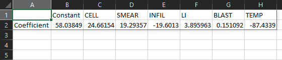
To perform a logistic regression between the occurrence of remission and the given factors, enter the formula =QRS.LOGISTIC.REGRESSION(C7:H33, B7:B33) in cell A1. The result contains 7 numbers. The first number is the regression constant. The remaining 6 numbers are the coefficients of the factors.
Labels and headers
=QRS.LOGISTIC.REGRESSION(C7:H33, B7:B33, "LABELS", TRUE, "NAMES", C6:H6)
Enter fullscreen mode
Exit fullscreen mode
To improve the presentation of the result, add "LABELS", TRUE and "NAMES", C6:H6 to the formula. The result now contains row labels and column headers.
Significance tests
=QRS.LOGISTIC.REGRESSION(C7:H33, B7:B33, "LABELS", TRUE, "NAMES", C6:H6, "LRTEST", "RAG")
Enter fullscreen mode
Exit fullscreen mode

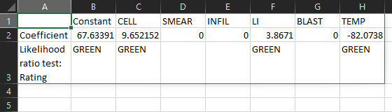
To determine the statistical significance of the factors, add "LRTEST", "RAG" to the formula. The result now contains red/amber/green ratings that summarize the likelihood ratio test for each factor.
The LI factor has a green rating. The other factors have red ratings. A green/amber rating means a factor is significant at the 5%/10% significance level. A red rating means a factor is not significant at the 10% significance level.
Please read the documentation to learn how to return the test statistic and p-value of the likelihood ratio test, as well as the corresponding results of the Wald test.
Significance levels
=QRS.LOGISTIC.REGRESSION(C7:H33, B7:B33, "LABELS", TRUE, "NAMES", C6:H6, "LRTEST", "RAG", "PGREEN", 0.3, "PRED", 0.35)
Enter fullscreen mode
Exit fullscreen mode

To change the significance levels from the default values of 5% and 10% to, say, 30% and 35%, add "PGREEN", 0.3 and "PRED", 0.35 to the formula. The TEMP factor now has a green rating too.
Manual factor selection
=QRS.LOGISTIC.REGRESSION(C7:H33, B7:B33, "LABELS", TRUE, "NAMES", C6:H6, "LRTEST", "RAG", "PGREEN", 0.3, "PRED", 0.35, "MASK", C5:H5)
Enter fullscreen mode
Exit fullscreen mode

To manually select only the LI and TEMP factors, enter 0, 0, 0, 1, 0, 1 in cells C5–H5 and add "MASK", C5:H5 to the formula. The excluded factors now have coefficients equal to zero.
Automatic factor selection
=QRS.LOGISTIC.REGRESSION(C7:H33, B7:B33, "LABELS", TRUE, "NAMES", C6:H6, "LRTEST", "RAG", "PGREEN", 0.3, "PRED", 0.35, "METHOD", "STEPWISE")
Enter fullscreen mode
Exit fullscreen mode
To automatically select factors using stepwise selection, remove "MASK", C5:H5 and add "METHOD", "STEPWISE" to the formula. The automatically selected factors are CELL, LI, and TEMP.
Please read the documentation to learn how to use forward selection or backward elimination instead, and how to control the significance levels for factor selection.
QRS.LOGISTIC.MODEL
You can calculate the probability modelled by a logistic regression in Excel using the QRS.LOGISTIC.MODEL function.
=QRS.LOGISTIC.MODEL(B$2:H$2, C7:H7)
Enter fullscreen mode
Exit fullscreen mode

Continuing from the example above, to calculate the probability of remission, enter the formula =QRS.LOGISTIC.MODEL(B$2:H$2, C7:H7) in cell I7, and copy the formula across cells I8–I33.
The probability of remission for Patient 01 is 72%. The probability for Patient 02 is 58%. The probability for Patient 03 is 10%, and so on.
Final remarks
If you find QRS.LOGISTIC.REGRESSION useful and would like to use it beyond your free trial period, you may purchase the right to use it indefinitely for as little as USD 29.00.