
Excel 2013 Office for business Spreadsheet Compare 2013 Spreadsheet Compare 2016 Spreadsheet Compare 2019 Spreadsheet Compare 2021 More…Less
Let’s say you have two Excel workbooks, or maybe two versions of the same workbook, that you want to compare. Or maybe you want to find potential problems, like manually-entered (instead of calculated) totals, or broken formulas. You can use Microsoft Spreadsheet Compare to run a report on the differences and problems it finds.
Important: Spreadsheet Compare is only available with Office Professional Plus 2013, Office Professional Plus 2016, Office Professional Plus 2019, or Microsoft 365 Apps for enterprise.
Open Spreadsheet Compare
On the Start screen, click Spreadsheet Compare. If you do not see a Spreadsheet Compare option, begin typing the words Spreadsheet Compare, and then select its option.
In addition to Spreadsheet Compare, you’ll also find the companion program for Access – Microsoft Database Compare. It also requires Office Professional Plus versions or Microsoft 365 Apps for enterprise.
Compare two Excel workbooks
-
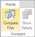
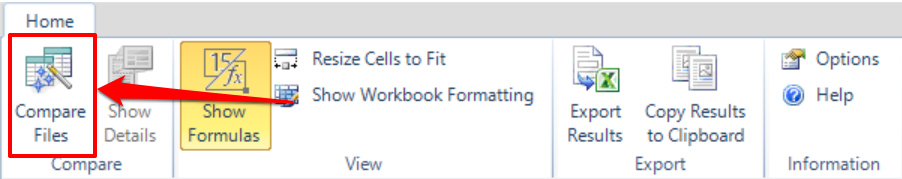
Click Home > Compare Files.

The Compare Files dialog box appears.
-
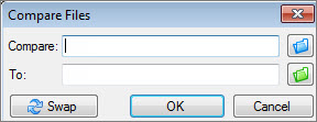
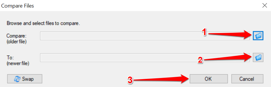
Click the blue folder icon next to the Compare box to browse to the location of the earlier version of your workbook. In addition to files saved on your computer or on a network, you can enter a web address to a site where your workbooks are saved.
-
Click the green folder icon next to the To box to browse to the location of the workbook that you want to compare to the earlier version, and then click OK.
Tip: You can compare two files with the same name if they’re saved in different folders.
-
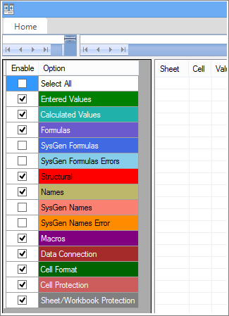
In the left pane, choose the options you want to see in the results of the workbook comparison by checking or unchecking the options, such as Formulas, Macros, or Cell Format. Or, just Select All.
-
Click OK to run the comparison.
If you get an «Unable to open workbook» message, this might mean one of the workbooks is password protected. Click OK and then enter the workbook’s password. Learn more about how passwords and Spreadsheet Compare work together.
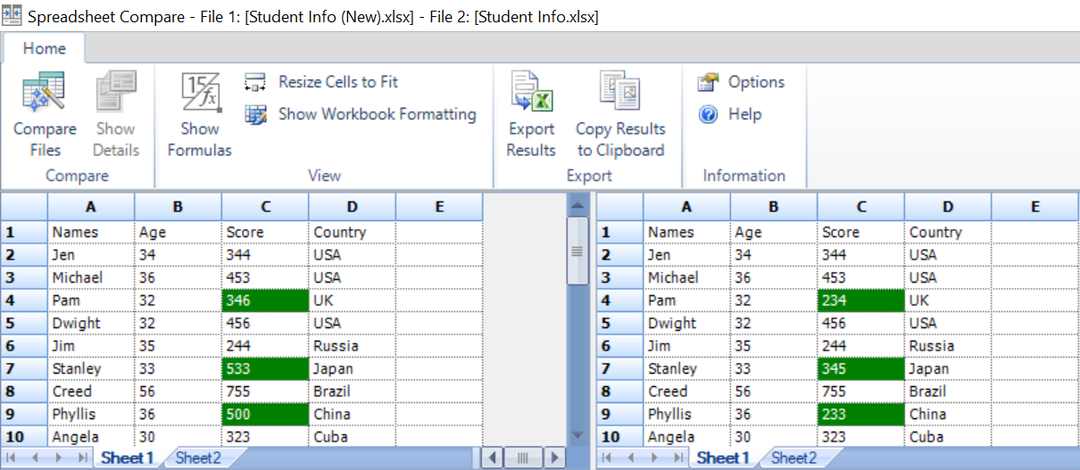
The results of the comparison appear in a two-pane grid. The workbook on the left corresponds to the «Compare» (typically older) file you chose and the workbook on the right corresponds to the «To» (typically newer) file. Details appear in a pane below the two grids. Changes are highlighted by color, depending on the kind of change.
Understanding the results
-
In the side-by-side grid, a worksheet for each file is compared to the worksheet in the other file. If there are multiple worksheets, they’re available by clicking the forward and back buttons on the horizontal scroll bar.
Note: Even if a worksheet is hidden, it’s still compared and shown in the results.
-
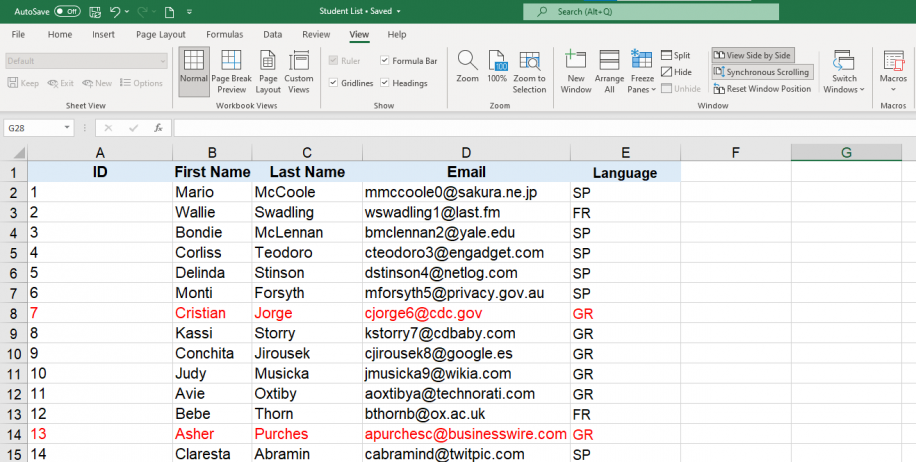
Differences are highlighted with a cell fill color or text font color, depending on the type of difference. For example, cells with «entered values» (non-formula cells) are formatted with a green fill color in the side-by-side grid, and with a green font in the pane results list. The lower-left pane is a legend that shows what the colors mean.
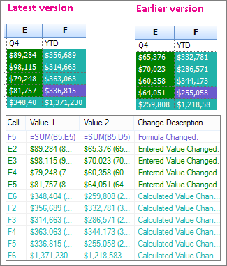
In the example shown here, results for Q4 in the earlier version weren’t final. The latest version of the workbook contains the final numbers in the E column for Q4.
In the comparison results, cells E2:E5 in both versions have a green fill that means an entered value has changed. Because those values changed, the calculated results in the YTD column also changed – cells F2:F4 and E6:F6 have a blue-green fill that means the calculated value changed.
The calculated result in cell F5 also changed, but the more important reason is that in the earlier version its formula was incorrect (it summed only B5:D5, omitting the value for Q4). When the workbook was updated, the formula in F5 was corrected so that it’s now =SUM(B5:E5).
-
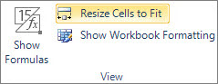
If the cells are too narrow to show the cell contents, click Resize Cells to Fit.
Excel’s Inquire add-in
In addition to the comparison features of Spreadsheet Compare, Excel 2013 has an Inquire add-in you can turn on that makes an «Inquire» tab available. From the Inquire tab, you can analyze a workbook, see relationships between cells, worksheets, and other workbooks, and clean excess formatting from a worksheet. If you have two workbooks open in Excel that you want to compare, you can run Spreadsheet Compare by using the Compare Files command.
If you don’t see the Inquire tab in Excel, see Turn on the Inquire add-in. To learn more about the tools in the Inquire add-in, see What you can do with Spreadsheet Inquire.
Next steps
If you have «mission critical» Excel workbooks or Access databases in your organization, consider installing Microsoft’s spreadsheet and database management tools. Microsoft Audit and Control Management Server provides powerful change management features for Excel and Access files, and is complemented by Microsoft Discovery and Risk Assessment Server, which provides inventory and analysis features, all aimed at helping you reduce the risk associated with using tools developed by end users in Excel and Access.
Also see Overview of Spreadsheet Compare.
Need more help?
One of the most common scenarios when working with Excel spreadsheets is having files with similar or duplicate data. The reasons for this could be many, but it usually involves spending a considerable amount of time checking complete files or separate worksheets manually.
This article will explain how to compare two or multiple Excel files, as well as two Excel sheets, for differences. To achieve this, we will describe how to use three useful methods to spot differences in a quick and easy way; these include side-by-side viewing, conditional formatting rules, and the =IF formula.
How to compare two Excel files using side-by-side view?
We will start by illustrating how to compare two Excel workbooks using the side-by-side view. However, we recommend using this method in case your dataset is not too large; if not, we recommend using one of the two methods outlined further on in this article. This is how you can compare two Excel files using the side-by-side viewing feature.
- 1. Open the two Excel workbooks you would like to compare and go to View > View Side by Side on any of the opened files.

How to compare two Excel files — View side by side
- 2. By default, Excel will place both files horizontally, as shown below.

How to compare two Excel files — Horizontal view
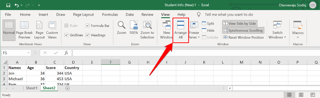
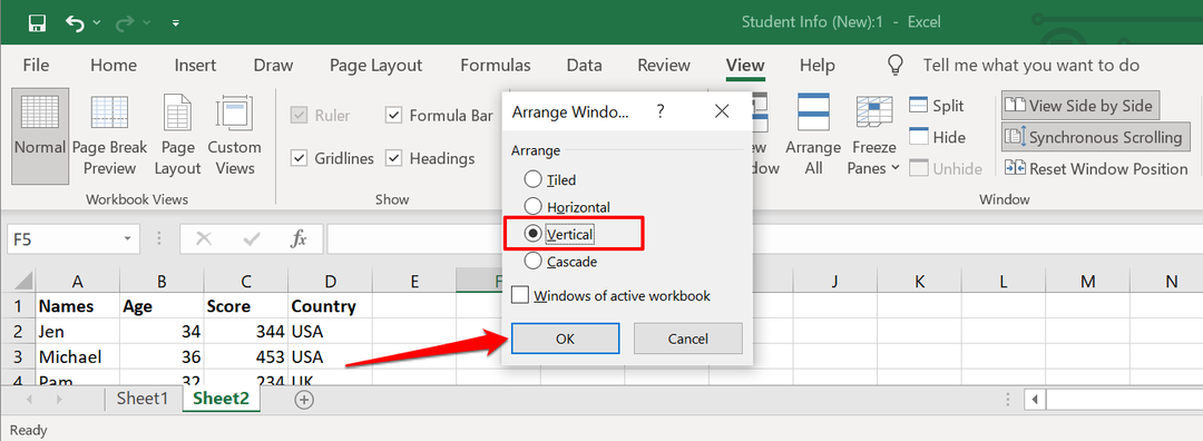
- 3. To arrange them vertically, click “Arrange All”, and then select “Vertical”.
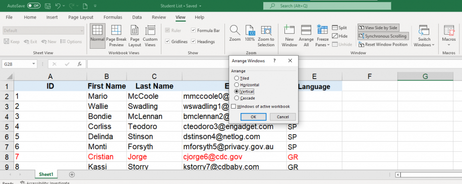
How to compare two Excel files — Arrange vertically
- 4. The two Excel files will now be arranged vertically, as shown below.

How to compare two Excel files — Vertical view
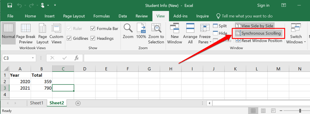
- 5. Make sure that the “Synchronous Scrolling” option is activated since this will allow you to scroll through the data on both files simultaneously and allow you to compare more easily. Although it activates automatically as soon as you enable the side-by-side view, you can also check that it’s activated in your toolbar within the “Window” group.
How to compare two Excel files — Synchronous Scrolling
Now that we know how easy it is to compare two Excel files, let’s see how we can apply this viewing method to Excel sheets.
How to Combine Multiple Excel Files Into One
Discover the most popular methods used to manually or automatically combine multiple Excel spreadsheets and data inputs into one master file
READ MORE

How to compare two Excel sheets using side-by-side view?
Sometimes, similar or duplicate data may appear within the same spreadsheet. IF you want to avoid having to switch from one sheet to another to compare the data, this is how you can quickly compare two Excel sheets side by side.
- 1. Open the Excel file where you would like to compare sheets. Then, go to View > New Window.

How to compare two Excel files — View New Window
- 2. You will now have the same Excel file open up in a different window, as shown below.

How to compare two Excel files — Same file in New Window
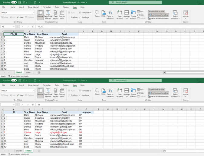
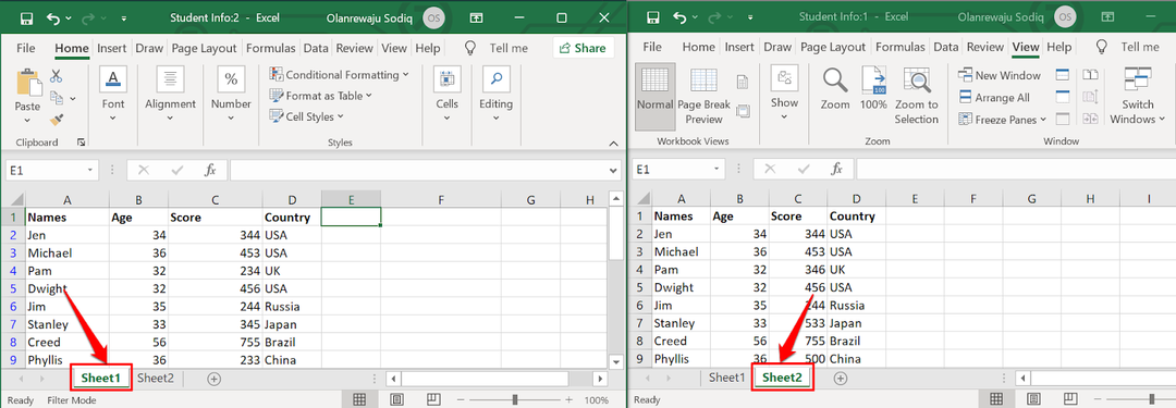
- 3. Select “View Side by Side” and make sure to select a different sheet on each file. As before, you can select vertical or horizontal viewing according to your preference.
How to compare two Excel files — Sheet 1 and 2
So far, you have seen how easy it is to compare two files and sheets on Excel. However, what if you would like to compare more than two files at the same time? This is how you can compare multiple Excel files using the side-by-side view.
How to compare multiple Excel files using side-by-side view?
Comparing multiple files for differences follows a similar process and will only take you a few simple steps.
- 1. Open all the Excel workbooks you would like to compare and go to View > View Side by Side. Select the file you want to start comparing with in the “Compare Side by Side” dialog box.

How to compare two Excel files — Compare side by side
- 2. Click “Arrange All” to view all the opened files at the same time.

How to compare two Excel files — Arrange All
- 3. Then, select the type of arrangement according to your preference. Here, I have chosen the “Tiled” arrangement.

How to compare two Excel files — Tiled arrangement
So far, these methods are useful in case your datasets are not too large and easily manageable. If you want to compare larger datasets for differences in values, the best way is to use the =IF formula or a conditional formatting rule. Let’s explore the =IF formula first.
How to compare two Excel sheets using a formula?
This is the most straightforward way to compare data between two Excel sheets. This formula will allow you to identify cells containing different values, and a comparative report will be generated in a new worksheet.
- 1. Open a new empty sheet in your Excel workbook and enter the following formula in cell A1: =IF(Sheet1!A1 <> Sheet2!A1, «Sheet1:»&Sheet1!A1&» vs Sheet2:»&Sheet2!A1, «»)

How to compare two Excel files — Enter IF formula
- 2. Grab the bottom-right corner of the formula cell, and drag down.

How to compare two Excel files — A1 cell comparison in Sheets
The formula will adapt to the column and row position it fills. This way, the formula in cell A1 compares to cell A1 in “Sheet1” and “Sheet2”; the formula in cell B1 will compare cell B1 in both sheets as well.
We will now turn to how to compare two Excel sheets by highlighting the differences. The best way to do so is by using the Excel conditional formatting feature.
How to compare two Excel sheets using conditional formatting?
When comparing two very similar and large datasets, the best and quickest way to spot differences in values is to highlight them using the conditional formatting feature.
- 1. Open the Excel sheets and select the range of data you would like to compare for differences. A quick way to do this is to click the upper-left cell and then Ctrl + Shift + End to extend the selection to the last cell containing values.

How to compare two Excel files — Select cell range
- 2. Go to Home > Conditional Formatting > New rule.

How to compare two Excel files — Create New Rule
- 3. Select the rule type “Use a formula to determine which cells to format” and enter the following, =A1<>Sheet1!A1. The Sheet name included in the formula corresponds to the sheet you are comparing with and not the one you are creating the rule in.

How to compare two Excel files — Use a formula
- 4. Once you’ve entered the formula, click “Format”, next to the “Preview” pane.

How to compare two Excel files — Format cells
- 5. Select how you would like to format the cells, i.e. according to “Number”, “Font”, “Border”, or “Fill”. We recommend highlighting with color fill, so we have chosen a color that will clearly stand out.

How to compare two Excel files — Format Fill
- 6. As you can see, Excel has highlighted the different cells in “Sheet 2” compared to “Sheet 1”.

How to compare two Excel files — Different cells highlighted
Now you know how to compare two or multiple Excel files and two sheets on your desktop. What if you want to compare and highlight differences in your Excel sheets online?
How to compare two Excel sheets and highlight differences online?
In case you don’t have Excel installed on your desktop or simply prefer to work online altogether, there are online tools that allow you to compare Excel files and sheets for differences.
Below, we provide a list of third-party tools that will allow you to compare Excel files and sheets online:
- Layer: Apart from allowing you to review spreadsheet changes and combine multiple spreadsheets into one, Layer offers additional features for file storage and management at a business level.
- Synkronizer Excel Compare: In addition to the features outlined in this article, it allows you to combine multiple Excel files into one, while maintaining unique values and avoiding duplicates.
- Ablebits Compare Sheets for Excel: This tool provides step-by-step guidance for efficient comparison and displays the differences found between sheets in the “Review Differences” mode for better management.
- Florencesoft DiffEngineX: Another excellent alternative that allows you to compare Excel files directly from Microsoft Outlook.
Want to Boost Your Team’s Productivity and Efficiency?
Transform the way your team collaborates with Confluence, a remote-friendly workspace designed to bring knowledge and collaboration together. Say goodbye to scattered information and disjointed communication, and embrace a platform that empowers your team to accomplish more, together.
Key Features and Benefits:
- Centralized Knowledge: Access your team’s collective wisdom with ease.
- Collaborative Workspace: Foster engagement with flexible project tools.
- Seamless Communication: Connect your entire organization effortlessly.
- Preserve Ideas: Capture insights without losing them in chats or notifications.
- Comprehensive Platform: Manage all content in one organized location.
- Open Teamwork: Empower employees to contribute, share, and grow.
- Superior Integrations: Sync with tools like Slack, Jira, Trello, and more.
Limited-Time Offer: Sign up for Confluence today and claim your forever-free plan, revolutionizing your team’s collaboration experience.
Conclusion
This article has shown you how to compare the data in two Excel files for differences. You can compare data between two files, two sheets, or multiple files using the side-by-side view for a quick and easy comparison. If your dataset is larger, you can apply the IF formula to compare two Excel sheets or use conditional formatting rules to highlight the differences.
Alternatively, for users that prefer to work online, there are platforms that can help you achieve this level of comparison in an online setting, for example, Layer. We also recommend reading our blog article on How To Combine Multiple Files into One as a great way to complete this data comparison process.
![]()
Download Article
Learn how to compare the values of two spreadsheets using synchronous scrolling, lookups, and more
![]()
Download Article
This article focuses on how to directly compare information between two different Excel files. Once you get to manipulating and comparing the information, you might want to use Look Up, Index, and Match to help your analysis.
-
1
Open the workbooks you need to compare. You can find these by opening Excel, clicking File then Open, and selecting two workbooks to compare from the menu that appears.
- Navigate to the folder where you have the Excel workbooks saved, select each workbook separately, and keep both workbooks open.
-
2
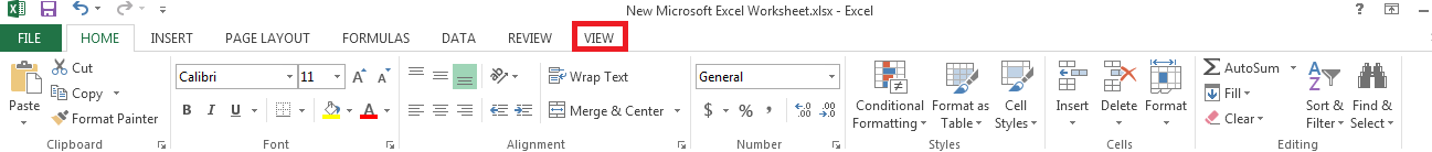
Click the View tab. Once you’ve opened one of the workbooks, you can click on the View tab in the top-center of the window.
Advertisement
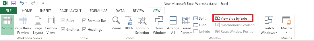
-
3
Click View Side by Side. This is located in the Window group of the ribbon for the View menu and has two sheets as its icon. This will pull up both worksheets into smaller windows stacked vertically.
- This option may not be readily visible under the View tab if you only have one workbook open in Excel.
- If there are two workbooks open, then Excel will automatically choose these as the documents to view side by side.
-
4
Click Arrange All. This setting lets you change the orientation of the workbooks when they’re displayed side-by-side.
- In the menu that pops up, you can select to have the workbooks Horizontal, Vertical, Cascade, or Tiled.
-
5
Enable Synchronous Scrolling. Once you have both worksheets open, click on Synchronous Scrolling (located under the View Side by Side option) to make it easier to scroll through both Excel files line-by-line to check for any differences in data manually.
-
6
Scroll through one workbook to scroll through both. Once Synchronous Scrolling is enabled, you’ll be able to easily scroll through both workbooks at the same time and compare their data more easily.


Advertisement
-
1
Open the workbooks you need to compare. You can find these by opening Excel, clicking File then Open, and selecting two workbooks to compare from the menu that appears.
- Navigate to the folder where you have the Excel workbooks saved, select each workbook separately and keep both workbooks open.
-
2
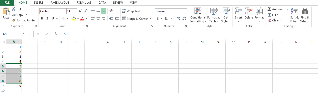
Decide on which cell you would like the user to select from. This is where a drop-down list will appear later.
-
3
Click on the cell. The border should darken.
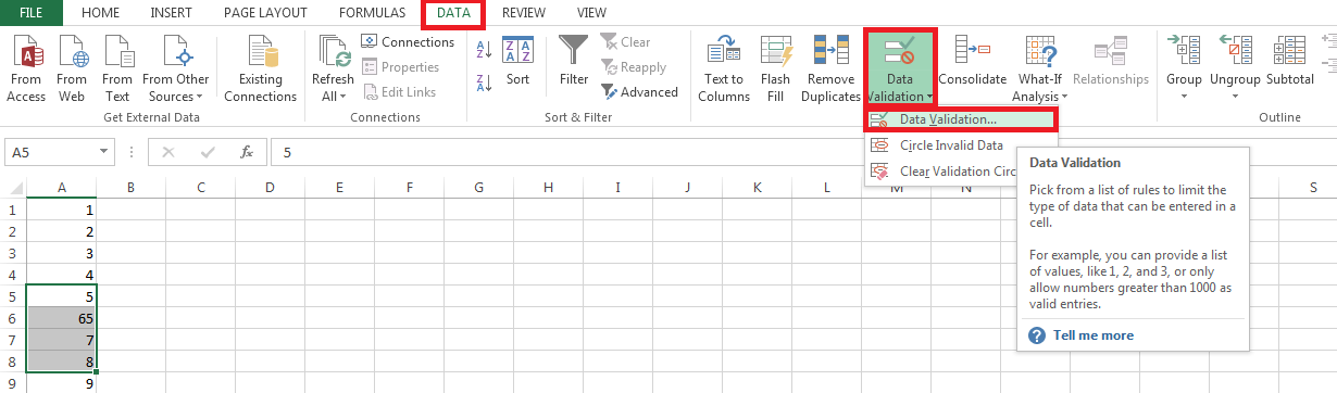
-
4
Click the DATA tab on the toolbar. Once you’ve clicked on it, select VALIDATION in the drop-down menu. A pop up should appear.
- If you’re using an older version of Excel, the DATA toolbar will pop up once you select the DATA tab and display Data Validation as the option instead of Validation.
-
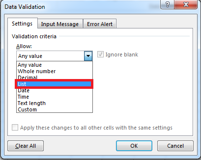
5
Click List in the ALLOW list.
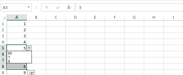
-
6
Click the button with the red arrow. This will let you pick your source (in other words, your first column), which will then be processed into data in the drop-down menu.
-
7
Select the first column of your list and press Enter. Click OK when the data validation window appears. You should see a box with an arrow on it, which will drop-down when you click the arrow.
-
8
Select the cell where you want the other info to show up.
-
9
Click the Insert and Reference tabs. In older versions of Excel, you can skip clicking the Insert tab and just click on the Functions tab to pull up the Lookup & Reference category.
-
10
Select Lookup & Reference from the category list.
-
11
Find Lookup in the list. When you double-click it, another box should appear and you can click OK.
-
12
Select the cell with the drop-down list for the lookup_value.
-
13
Select the first column of your list for the Lookup_vector.
-
14
Select the second column of your list for the Result_vector.
-
15
Pick something from the drop-down list. The info should automatically change.


Advertisement
-
1
Open your browser and go to https://www.xlcomparator.net. This will take you to XL Comparator’s website, where you can upload two Excel workbooks for comparison.
-
2
Click Choose File. This will open a window where you can navigate to one of the two Excel documents you want to compare. Make sure to select a file for both fields.
-
3
Click Next > to continue. Once you’ve selected this, a pop-up message should appear at the top of the page letting you know that the file upload process has begun and that larger files will take longer to process. Click Ok to close this message.
-
4
Select the columns you want to be scanned. Underneath each file name is a drop-down menu that says Select a column. Click on the drop-down menu for each file to select the column you want to be highlighted for comparison.
- Column names will be visible when you click the drop-down menu.
-
5
Select contents for your result file. There are four options with bubbles next to them in this category, one of which you’ll need to select as the formatting guidelines for your result document.
-
6
Select the options to ease column comparison. In the bottom cell of the comparison menu, you’ll see two more conditions for your document comparison: Ignore uppercase/lowercase and Ignore «spaces» before and after values. Click the checkbox for both before proceeding.
-
7
Click Next > to continue. This will take you to the download page for your result document.
-
8
Download your comparison document. Once you’ve uploaded your workbooks and set your parameters, you’ll have a document showing comparisons between data in the two files available for download. Click the underlined Click here text in the Download the comparison file box.
- If you want to run any other comparisons, click New comparison in the bottom-right corner of the page to restart the file upload process.


Advertisement
-
1
Locate your workbook and sheet names.
- In this case, we use three example workbooks located and named as follows:
- C:CompareBook1.xls (containing a sheet named “Sales 1999”)
- C:CompareBook2.xls (containing a sheet named “Sales 2000”)
- Both workbooks have the first column “A” with the name of the product, and the second column “B” with the amount sold each year. The first row is the name of the column.
- In this case, we use three example workbooks located and named as follows:
-
2
Create a comparison workbook. We will work on Book3.xls to do a comparison and create one column containing the products, and one with the difference of these products between both years.
- C:CompareBook3.xls (containing a sheet named “Comparison”)
-
3
Place the title of the column. Only with “Book3.xls” opened, go to cell “A1” and type:
- =’C:Compare[Book1.xls]Sales 1999′!A1
- If you are using a different location replace “C:Compare” with that location. If you are using a different filename remove “Book1.xls” and add your filename instead. If you are using a different sheet name replace “Sales 1999” with the name of your sheet. Beware not to have the file you are referring (“Book1.xls”) opened: Excel may change the reference you are adding if you have it open. You’ll end up with a cell that has the same content as the cell you referred to.
-
4
Drag down cell “A1” to list all products. Grab it from the bottom right square and drag it, copying all names.
-
5
Name the second column. In this case, we call it “Difference” in «B1».
-
6
(For example) Estimate the difference of each product. In this case, by typing in cell “B2”:
- =’C:Compare[Book2.xls]Sales 2000′!B2-‘C:Compare[Book1.xls]Sales 1999’!B2
- You can do any normal Excel operation with the referred cell from the referred file.
-
7
Drag down the lower corner square and get all differences, as before.


Advertisement
Ask a Question
200 characters left
Include your email address to get a message when this question is answered.
Submit
Advertisement
-
Remember it is important to have the referred files closed. If you have them opened, Excel may override what you type in the cell, making it impossible to access the file afterward (unless again you have it open).
Thanks for submitting a tip for review!
Advertisement
About This Article
Article SummaryX
1. Open two Excel documents.
2. Click the View tab.
3. Click View Side by Side.
4. Click Arrange All to adjust display.
5. Enable Synchronous Scrolling.
Did this summary help you?
Thanks to all authors for creating a page that has been read 233,724 times.
Is this article up to date?
Watch Video – How to Compare Two Excel Sheets for Differences
Comparing two Excel files (or comparing two sheets in the same file) can be tricky as an Excel workbook only shows one sheet at a time.
This becomes more difficult and error-prone when you have a lot of data that needs to be compared.
Thankfully, there are some cool features in Excel that allow you to open and easily compare two Excel files.
In this Excel tutorial, I will show you multiple ways to compare two different Excel files (or sheets) and check for differences. The method you choose will depend on how your data is structured and what kind of comparison you’re looking for.
Let’s get started!
Compare Two Excel Sheets in Separate Excel Files (Side-by-Side)
If you want to compare two separate Excel files side by side (or two sheets in the same workbook), there is an in-built feature in Excel to do this.
It’s the View Side by Side option.
This is recommended only when you have a small dataset and manually comparing these files is likely to be less time-consuming and error-prone. If you have a large dataset, I recommend using the conditional method or the formula method covered later in this tutorial.
Let’s see how to use this when you have to compare two separate files or two sheets in the same file.
Suppose you have two files for two different months and you want to check what values are different in these two files.
By default, when you open a file, it’s likely to take up your entire screen. Even if you reduce the size, you always see one Excel file at the top.
With the view side-by-side option, you can open two files and then arrange these horizontally or vertically. This allows you to easily compare the values without switching back and forth.
Below are the steps to align two files side by side and compare them:
- Open the files that you want to compare.
- In each file, select the sheet that you want to compare.
- Click the View tab

- In the Windows group, click on the ‘View Side by Side’ option. This becomes available only when you have two or more Excel files open.


As soon as you click on the View side by side option, Excel will arrange the workbook horizontally. Both of the files will be visible, and you’re free to edit/compare these files while they are arranged side by side.

In case you want to arrange the files vertically, click on the Arrange All option (in the View tab).

This will open the ‘Arrange Windows’ dialog box where you can select ‘Vertical’.

At this point, if you scroll down in one of the worksheets, the other one would remain as is. You can change this so that when you scroll in one sheet, the other also scrolls at the same time. This makes it easier to do a line by line comparison and spot any differences.
But to do this, you need to enable Synchronous Scrolling.
To enable Synchronous Scrolling, click on the View tab (in any of the workbooks) and then click on the Synchronous Scrolling option. This is a toggle button (so if you want to turn it off, simply click on it again).

Comparing Multiple Sheets in Separate Excel Files (Side-by-Side)
With the ‘View Side by Side’ option, you can only compare two Excel file at one go.
In case you have multiple Excel files open, when you click on the View Side by Side option, it will show you a ‘Compare Side by Side’ dialog box, where you can choose which file you want to compare with the active workbook.
In case you want to compare more than two files at one go, open all these files and then click on the Arrange All option (it’s in the View tab).
In the Arrange Windows dialog box, select Vertical/Horizontal and then click OK.
This will arrange all the open Excel files in the selected order (vertical or horizontal).
Compare Two Sheets (Side-by-Side) in the Same Excel Workbook
In case you want to compare two separate sheets in the same workbook, you can’t use the View side by side feature (as it works for separate Excel files only).
But you can still do the same side-by-side comparison.
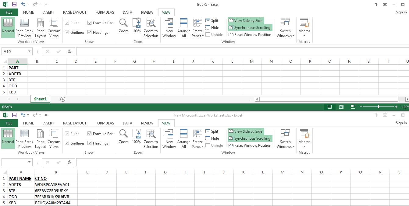
This is made possible by the ‘New Windows’ feature in Excel, that allows you to open two instances on the same workbook. Once you have two instances open, you can arrange these side by side and then compare these.
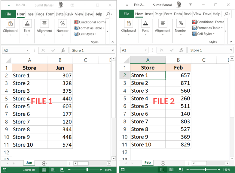
Suppose you have an Excel workbook that has two sheets for two different months (Jan and Feb) and you want to compare these side by side to see how the sales per store have changed:

Below are the steps to compare two sheets in Excel:
- Open the workbook that has the sheets that you want to compare.
- Click the View tab
- In the Window group, click on the ‘New Window’ option. This opens the second instance of the same workbook.
- In the ‘View’ tab, click on ‘Arrange All’. This will open the Arrange Windows dialog box

- Select ‘Vertical’ to compare data in columns (or select Horizontal if you want to compare data in rows).

- Click OK.
The above steps would arrange both the instances of the workbook vertically.
At this point in time, both the workbooks would have the same worksheet selected. In one of the workbooks, select the other sheet that you want to compare with the active sheet.
How does this work?
When you click on New Window, it opens the same workbook again with a slightly different name. For example, if your workbook name is ‘Test’ and you click on New Window, it will name the already open workbook ‘Test – 1’ and the second instance as ‘Test – 2’.
Note that these are still the same workbook. If you make any changes in any of these workbooks, it would be reflected in both.
And when you close any one instance of the open file, the name would revert back to the original.
You can also enable synchronous scrolling if you want (by clicking on the ‘Synchronous Scrolling’ option in the ‘View’ tab)
Compare Two Sheets and Highlight Differences (Using Conditional Formatting)
While you can use the above method to align the workbooks together and manually go through the data line by line, it’s not a good way in case you have a lot of data.
Also, doing this level of comparison manually can lead to a lot of errors.
So instead of doing this manually, you can use the power of Conditional Formatting to quickly highlight any differences in the two Excel sheets.
This method is really useful if you have two versions in two different sheets and you want to quickly check what has changed.
Note that you CAN NOT compare two sheets in different workbooks.
Since Conditional Formatting can not refer to an external Excel file, the sheets you need to compare needs to be in the same Excel workbook. In case these aren’t, you can copy a sheet from the other file to the active workbook and then make this comparison.
For this example, suppose you have a dataset as shown below for two months (Jan and Feb) in two different sheets and you want to quickly compare the data in these two sheets and check if the prices of these items have changed or not.

Below are the steps to do this:
- Select the data in the sheet where you want to highlight the changes. Since I want to check how prices have changed from Jan to Feb, I have selected the data in the Feb sheet.
- Click the Home tab

- In the Styles group, click on ‘Conditional Formatting’

- In the options that show up, click on ‘New Rule’

- In the ‘New Formatting Rule’ dialog box, click on ‘Use a formula to determine which cells to format’

- In the formula field, enter the following formula: =B2<>Jan!B2
- Click the Format button
- In the Format Cells dialog box that shows up, click on the ‘Fill tab’ and select the color in which you want to highlight the mismatched data.

- Click OK
- Click OK


The above steps would instantly highlight any changes in the dataset in both the sheets.

How does this work?
Conditional formatting highlights a cell when the given formula for that cell returns a TRUE. In this example, we are comparing each cell in one sheet with the corresponding cell in the other sheet (done using the not equal to operator <> in the formula).
When conditional formatting finds any difference in the data, it highlights that in the Jan sheet (the one in which we have applied the conditional formatting.
Note that I have used relative reference in this example (A1 and not $A$1 or $A1 or A$1).
When using this method to compare two sheets in Excel, remember the following;
- This method is good to quickly identify differences, but you can’t use it on an on-going basis. For example, if I enter a new row in any of the datasets (or delete a row), it would give me incorrect results. As soon as I insert/delete the row, all subsequent rows are considered as different and highlighted accordingly.
- You can only compare two sheets in the same Excel file
- You can only compare the value (not the difference in formula or formatting).
Compare Two Excel Files/Sheets And Get The Differences Using Formula
If you’re only interested in quickly comparing and identifying the differences between two sheets, you can use a formula to fetch only those values that are different.
For this method, you will need to have a separate worksheet where you can fetch the differences.
This method would work if want to compare two separate Excel workbook or worksheets in the same workbook.
Let me show you an example where I am comparing two datasets in two sheets (in the same workbook).
Suppose you have the dataset as shown below in a sheet called Jan (and similar data in a sheet called Feb), and you want to know what values are different.
To compare the two sheets, first, insert a new worksheet (let’s call this sheet ‘Difference’).
In cell A1, enter the following formula:
=IF(Jan!A1<>Feb!A1,"Jan Value:"&Jan!A1&CHAR(10)&"Feb Value:"&Feb!A1,"")

Copy and paste this formula for a range so that it covers the entire dataset in both the sheets. Since I have a small dataset, I will only copy and paste this formula in A1:B10 range.
The above formula uses an IF condition to check for differences. In case there is no difference in the values, it will return blank, and in case there is a difference, it will return the values from both the sheets in separate lines in the same cell.
The good thing with this method is that it only gives you the differences and show you exactly what the difference is. In this example, I can easily see that the price in cell B4 and B8 are different (as well as the exact values in these cells).
Compare Two Excel Files/Sheets And Get The Differences Using VBA
If you need to compare Excel files or sheets quite often, it’s a good idea to have a ready Excel macro VBA code and use it whenever you need to make the comparison.
You can also add the macro to the Quick Access Toolbar so that you can access with a single button and instantly know what cells are different in different files/sheets.
Suppose you have two sheets Jan and Feb and you want to compare and highlight differences in the Jan sheet, you can use the below VBA code:
Sub CompareSheets()
Dim rngCell As Range

For Each rngCell In Worksheets("Jan").UsedRange

    If Not rngCell = Worksheets("Feb").Cells(rngCell.Row, rngCell.Column) Then
        rngCell.Interior.Color = vbYellow
    End If

Next rngCell

End Sub
The above code uses the For Next loop to go through each cell in the Jan sheet (the entire used range) and compares it with the corresponding cell in the Feb sheet. In case it finds a difference (which is checked using the If-Then statement), it highlights those cells in yellow.
You can use this code in a regular module in the VB Editor.
And if you need to do this often, it’s better to save this code in the Personal Macro workbook and then add it to the Quick Access toolbar. In those ways, you will be able to do this comparison with a click of a button.
Here are the steps to get the Personal Macro Workbook in Excel (it’s not available by default so you need to enable it).
Here are the steps to save this code in the Personal Macro Workbook.
And here you will find the steps to add this macro code to the QAT.
Using a Third-Party Tool – XL Comparator
Another quick way to compare two Excel files and check for matches and differences is by using a free third-party tool such as XL Comparator.
This is a web-based tool where you can upload two Excel files and it will create a comparison file that will have the data that is common (or different data based on what option you selected.
Suppose you have two files that have customer datasets (such as name and email address), and you want to quickly check what customers are there is file 1 and not in file 2.
Below is how you compare two Excel files and create a comparison report:
- Open https://www.xlcomparator.net/
- Use the Choose file option to upload two files (maximum size of each file can be 5MB)
- Click on the Next button.
- Select the common column in both these files. The tool will use this common column to look for matches and differences
- Select one of the four options, whether you want to get matching data or different data (based on File 1 or File 2)
- Click on Next
- Download the comparison file which will have the data (based on what option you selected in step 5)
Below is a video that shows how XL Comparator tool works.
One concern you may have when using a third-party tool to compare Excel files is about privacy.
If you have confidential data and privacy is really important for it, it’s better to use other methods shown above.
Note that the XL Comparator website mentions that they delete all the files after 1 hour of doing the comparison.
These are some of the methods you can use to compare two different Excel files (or worksheets in the same Excel file). Hope you found this Excel tutorial useful.
You may also like the following Excel tutorials:
- How to Compare Two Columns in Excel (for matches & differences)
- How to Remove Duplicates in Excel
- How to Compare Text in Excel (Easy Formulas)
- Split Each Excel Sheet Into Separate Files (Step-by-Step)
- Combine Data from Multiple Workbooks in Excel
- Combine Data From Multiple Worksheets into a Single Worksheet in Excel
- How to Compare Dates in Excel (Greater/Less Than, Mismatches)
Compare two Excel workbooks
- Click Home > Compare Files.
- Click the blue folder icon next to the Compare box to browse to the location of the earlier version of your workbook.
Contents
- 1 Can I compare two Excel spreadsheets for differences?
- 2 How do I compare 2 Excel files?
- 3 How do you compare data in two Excel sheets for matches?
- 4 How do you compare two Excel sheets and remove duplicates?
- 5 How do you set up a comparison spreadsheet?
- 6 Where can I find spreadsheet comparison?
- 7 How do I compare two Excel columns for differences?
- 8 How do you use the Match function in Excel?
- 9 How do I remove duplicates in two columns in Excel?
- 10 What is Vlookup in Excel?
- 11 How do I compare two columns in Excel to match?
- 12 How do I compare two columns in Excel for partial matches?
- 13 How do I see all matches in Excel?
- 14 How do you find exact match in Excel?
- 15 How do you compare two columns in Excel and return a value?
- 16 How do I filter duplicates in Excel?
- 17 How do I find duplicates in Excel without deleting them?
- 18 How do you do a VLOOKUP for beginners?
- 19 What is not possible with VLOOKUP?
Can I compare two Excel spreadsheets for differences?
With the ‘View Side by Side’ option, you can only compare two Excel file at one go. In case you have multiple Excel files open, when you click on the View Side by Side option, it will show you a ‘Compare Side by Side’ dialog box, where you can choose which file you want to compare with the active workbook.
Compare 2 Excel workbooks
- Open the workbooks you want to compare.
- Go to the View tab, Window group, and click the View Side by Side button. That’s it!
How do you compare data in two Excel sheets for matches?
Select both columns of data that you want to compare. On the Home tab, in the Styles grouping, under the Conditional Formatting drop down choose Highlight Cells Rules, then Duplicate Values. On the Duplicate Values dialog box select the colors you want and click OK. Notice Unique is also a choice.
How do you compare two Excel sheets and remove duplicates?
Remove Duplicates
- Open a workbook with two worksheets you’d like to merge.
- Select all data in the first worksheet, and then press “Ctrl-C” to copy it to the clipboard.
- Select all data in the new workbook, and then click the Data tab’s “Remove Duplicates” command, located in the Data Tools command group.
How do you set up a comparison spreadsheet?
To access the Spreadsheet Compare Add In, click on the Windows icon in the lower left of your task bar, and search for Spreadsheet Compare. You will be taken to a sort of mission control for comparing spreadsheets.
Where can I find spreadsheet comparison?
To Use Spreadsheet Compare
- Find and launch the app by clicking Start then typing ‘Spreadsheet Compare’.
- Click Compare Files. The Compare Files dialog appears.
- Click the folder icon to select the older and newer files, then click OK.
How do I compare two Excel columns for differences?
Compare Two Columns and Highlight Matches
- Select the entire data set.
- Click the Home tab.
- In the Styles group, click on the ‘Conditional Formatting’ option.
- Hover the cursor on the Highlight Cell Rules option.
- Click on Duplicate Values.
- In the Duplicate Values dialog box, make sure ‘Duplicate’ is selected.
How do you use the Match function in Excel?
The MATCH function searches for a specified item in a range of cells, and then returns the relative position of that item in the range. For example, if the range A1:A3 contains the values 5, 25, and 38, then the formula =MATCH(25,A1:A3,0) returns the number 2, because 25 is the second item in the range.
How do I remove duplicates in two columns in Excel?
Remove Duplicates from Multiple Columns in Excel
- Select the data.
- Go to Data –> Data Tools –> Remove Duplicates.
- In the Remove Duplicates dialog box: If your data has headers, make sure the ‘My data has headers’ option is checked. Select all the columns except the Date column.
What is Vlookup in Excel?
VLOOKUP stands for ‘Vertical Lookup’. It is a function that makes Excel search for a certain value in a column (the so called ‘table array’), in order to return a value from a different column in the same row.
How do I compare two columns in Excel to match?
Excel allows a user to compare two columns by using the SUMPRODUCT function.
Using the SUMPRODUCT to Count Matches Between Two Columns
- Select cell F2 and click on it.
- Insert the formula: =SUMPRODUCT(–(B3:B12 = C3:C12))
- Press enter.
How do I compare two columns in Excel for partial matches?
Compare Two Columns and Highlight Matches
- Select the range which contains names.
- Go to the Home tab and choose the Styles group.
- Select the Highlight cell Rules option then click on the Duplicate values.
- The Duplicate Values dialog box will appear.
- Apply your favorite style using the drop-down list.
- Click OK.
How do I see all matches in Excel?
1. Select a blank cell to output the first matched instance, enter the below formula into it, and then press the Ctrl + Shift + Enter keys simultaneously. Note: In the formula, B2:B11 is the range which the matched instances locate in. A2:A11 is the range contains the certain value you will list all instances based on.
How do you find exact match in Excel?
Excel EXACT Function
- Summary.
- Compare two text strings.
- A boolean value (TRUE or FALSE)
- =EXACT (text1, text2)
- text1 – The first text string to compare.
- The EXACT function compares two text strings in a case-sensitive manner.
How do you compare two columns in Excel and return a value?
Option one
- Go to cell E2 and enter the formula =IF(ISNUMBER(MATCH(D2,$A$2:$A$20,0)),INDEX(Sheet5!$B$2:$B$20,MATCH(Sheet5!
- Press ENTER key to get the matching content on the E2.
- Copy the formula to the rest of the cells using the Autofill feature or drag the fill handle down to cells you want to copy the formula.
How do I filter duplicates in Excel?
In Excel, there are several ways to filter for unique values—or remove duplicate values:
- To filter for unique values, click Data > Sort & Filter > Advanced.
- To remove duplicate values, click Data > Data Tools > Remove Duplicates.
How do I find duplicates in Excel without deleting them?
If you simply want to find duplicates, so you can decide yourself whether or not to delete them, your best bet is highlighting all duplicate content using conditional formatting. Select the columns you want to check for duplicate information, and click Home > Highlight Cell Rules > Duplicate Values.
How do you do a VLOOKUP for beginners?
- In the Formula Bar, type =VLOOKUP().
- In the parentheses, enter your lookup value, followed by a comma.
- Enter your table array or lookup table, the range of data you want to search, and a comma: (H2,B3:F25,
- Enter column index number.
- Enter the range lookup value, either TRUE or FALSE.
What is not possible with VLOOKUP?
Problem: The lookup value is not in the first column in the table_array argument. One constraint of VLOOKUP is that it can only look for values on the left-most column in the table array. If your lookup value is not in the first column of the array, you will see the #N/A error.
Affiliate disclosure: In full transparency – some of the links on our website are affiliate links, if you use them to make a purchase we will earn a commission at no additional cost for you (none whatsoever!).
By being an Excel wizard, you can indeed save a heck lot of your time and can do complex tasks easily. Did you know that you can compare excel files with some simple tweaks and options? If not, then this article is for you.
So, do you want to know how to compare two excel files? If yes then you are certainly at the right place. Comparing the two data graphically can also make the data more representable and easy to understand. You can create charts to show the data. Here is how to create charts in Excel. So, let’s get started with the same:
How to Compare Two Excel Files?
Method 1: Using compare feature.
If you are using Microsoft Excel 2013 edition, then you can easily access the compare feature. So, as it is clearly stated that the prerequisites of this method are Excel 2013, and two workbooks that you want to compare. This is it.
Step #1: You know the obvious step, right. You need to open both the workbooks on Excel and then proceed to the next steps which will guide you how to compare two excel files?
Step #2: Once you have both the workbooks opened in your excel dashboards then you require navigating to the inquire tab. Once you are there, then you need to select “Compare Files” option from the ribbon itself.
This will open a “Select files to compare” dialog box for you.
On the dialog box, all that you require is to select both the Excel files that you want to compare. You will see two fields as “Compare” and “To”.
Step #3: After successfully going through the previous steps, you now require clicking on “Compare” button which is positioned at the bottom of the “Select files to compare” dialog box.
Now, your part has come to an end. Excel will now do the rest for you. It will highlight all the differences like formulas, data, formatting and others. There is a total of fourteen factors where the Excel compare tool pays utmost heed to. To be more precise, it highlights the difference based on these 14 factors. However, you can certainly choose what differences should be emphasized and what not.
The fourteen areas are:
1: Macros.
2: Entered Values.
3: Formulas.
4: Calculated Values.
5: SysGen Formulas.
6: Structural.
7: Names.
8: SysGen Formula errors.
9: SysGen Names.
10: SysGen names errors.
11: Cell format.
12: Cell Protection.
13: Sheet/Workbook protection.
14: Data connection.
This way you can easily compare two excel files. You can also compare two excel data using Bar graphs. Bar graphs can make the representation more appealing. If you don’t know how to make a bar graph, see the link.
Method 2: Using Side by Side.
Unlike the previous method which does the needful for you, this method will allow you to compare your workbooks manually. You will have to check manually for the all the differences by scrolling down for each and every page of the two workbooks. This method will also work on the previous version of Microsoft Excel. So, let’s get started:
Step #1: In this very first step, you need to launch both the workbooks. Once you are done with the same, then you are ready to go to the next steps.
![]()
Step #2: Now, from the top navigation bar, you need to navigate to the “View” tab. Once you have navigated the same then, you need to click on it.
Step #3: From the “view” ribbon, you now need to locate “View Side by Side”. The “view side by side” option can be seen in the “Window” section of the view tab. This will open a dialog box for you. On the dialog box, you have to select the workbook which you want to compare with the currently active workbook. Once you are done with the same, then all that you require is to click on “OK” button.
Step #4: The previous step of yours will open the two workbooks side by side. Now, you can manually scroll and can easily spot the differences. When you scroll the window, both the workbooks will be scrolled together in sync. This way you can easily compare the two file and spot the contrast.
Additionally, if you want to turn off the synchronous scrolling, then you can go for the “Synchronous Scrolling” option from the Window section and turn it off.
Step #5: The moment you are done with the comparison of two Excel files then you now need to turn off the View side by side option and revert to the normal mode. You can easily do this by clicking again on “View Side by Side” option and this way you will be back to the normal mode.
[Additional Information]: How to create drop-down menu in excel?
It may seem a little off topic, but we thought that you might be interested in know how to create a drop-down menu in Excel? This is why you are brought to this additional information section. So, here we go:
Step #1: Open Excel sheet and select the cell or range for which you want to drop-down list. You can even select multiple cells or even a full column. If you want to select a handful of columns then you will have to press control while selecting the desired ones.
Step #2: After step #1, you now need to select Excel data validation. For this, you will have to follow the following route: Data tab -> Data tools. This will result in an appearance of a list from which you are required to select “Data Validation.”
Step #3: A new window will appear after you select “Data Validation” in the previous step. From the window, you have to select “list” in the allow box.
After this type those entities which you want to appear on your list.
Make sure that you have checked the box next to which “In-cell dropdown” is written.
Step #4: Now, as the final step, you are required to click on OK and this way you can easily create a drop-down menu in excel.
We hope that this might be of some help for you. You can also compare two datas by calculating the average. Here is you can calculate the average in Excel.
This brought us to the end of this article on “How to compare two excel sheets?”
Do you know any other method by which you can easily compare two excel sheets? If yes, then do tell us by dropping a line through the comments section. Your addition is highly valuable.
If you liked this article then do not forget to share it. Thank you.
Есть два одноименных Файлы Excel в разных папках на вашем компьютере. Как определить, являются ли файлы дубликатами или разными версиями одной книги Excel? В этом руководстве мы покажем вам, как сравнить два файла Excel, даже если на вашем компьютере не установлен Excel.
Эти инструменты сравнения могут помочь вам обнаружить несогласованные данные, устаревшие значения, неверные формулы, неправильные вычисления и другие проблемы на вашем листе Excel.
Оглавление
1. Сравните два листа Excel: просмотр бок о бок
Если вы можете быстро просмотреть данные на листе, откройте их в отдельном окне и выполните параллельное сравнение с помощью функции Excel «Просмотр бок о бок».
- Откройте файл Excel, содержащий оба листа, перейдите к Вид вкладка и выберите Новое окно.

- В новом окне выберите или переключиться на (второй) рабочий лист вы хотите сравнить.
Измените размер или порядок окон, чтобы оба листа отображались на экране компьютера бок о бок. Опять же, этот метод лучше всего подходит для сравнения листов Excel с несколькими строками или столбцами.
- Если вы предпочитаете использовать инструмент сравнения Excel для размещения обоих окон бок о бок, проверьте вкладку «Просмотр» и выберите Просмотр бок о бок значок.

Excel сразу же расположит оба листа по горизонтали на экране вашего компьютера. Сравнивать листы в этом альбомном режиме может быть немного сложно, поэтому перейдите к следующему шагу, чтобы изменить ориентацию на вертикальное / книжное расположение.
- Снова перейдите на вкладку «Просмотр» и выберите Упорядочить все.
- Выбирать Вертикальный в окне «Упорядочить» и выберите В ПОРЯДКЕ.
В результате оба листа будут располагаться на экране рядом друг с другом. Есть еще один параметр, который нужно включить, чтобы упростить сравнение.
- Кран Синхронная прокрутка и убедитесь, что он выделен. Это позволяет прокручивать оба листа одновременно, обеспечивая синхронное построчное сравнение вашего набора данных.
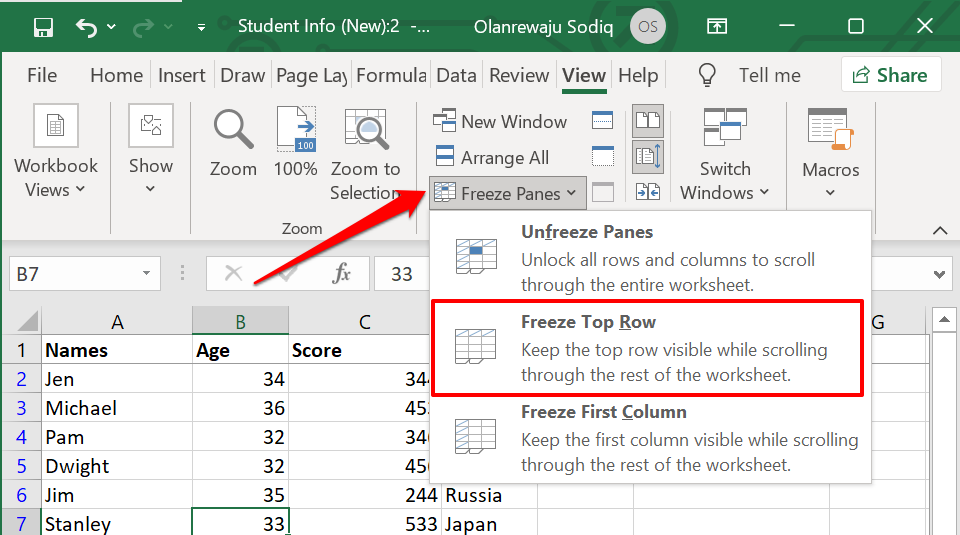
Если верхние строки обоих листов являются заголовками, убедитесь, что вы закрепили их, чтобы они не перемещались вместе с остальной частью набора данных при прокрутке.
- Выбирать Замерзшие оконные стекла и выберите Закрепить верхнюю строку. Повторите этот шаг для второго листа.
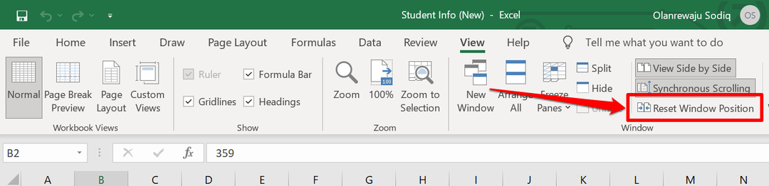
- Выбирать Сбросить положение окна, чтобы вернуть ориентацию сравнения к альбомному формату.
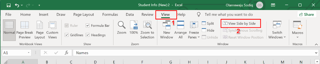
- Когда вы закончите сравнение, выберите Просмотр бок о бок чтобы вернуть листы к исходным размерам.
Теперь вы можете просматривать оба листа и сравнивать их построчно. Основным преимуществом этой функции является то, что она встроена во все версии Excel. Однако вам все равно придется проделать кучу работы, например, выделить ячейки с разными фигурами, макросами, формулами и т. Д.
2. Сравните два файла Excel с помощью онлайн-инструментов
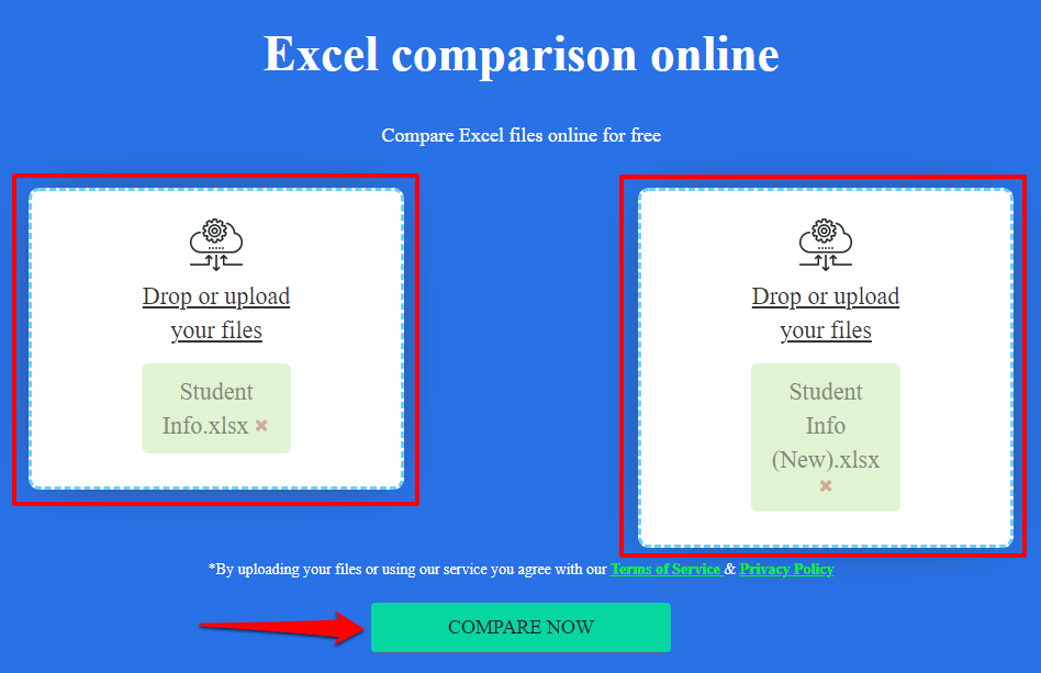
Существуют веб-инструменты, предлагающие услуги сравнения Excel. Вы найдете эти инструменты полезными, если на вашем компьютере не установлен Excel. Этот Инструмент сравнения Excel от Aspose — хороший веб-инструмент для сравнения двух файлов Excel.
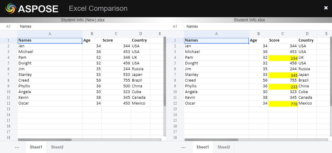
Загрузите первый (основной) файл Excel в первое поле, перетащите другой файл во второе поле и выберите Сравнить сейчас кнопка.
Если в файлах несколько листов, выберите листы, которые вы хотите сравнить, на вкладке «Листы». Если на обоих листах есть ячейки с разными значениями или содержимым, инструмент сравнения Aspose Excel выделит различия желтым цветом.
Ограничение этих веб-инструментов заключается в том, что они в основном выделяют разные значения. Они не могут выделить несоответствующие формулы, расчеты и т. Д.
3. Сравните два файла Excel с помощью функции «Сравнение электронных таблиц»
Таблица сравнения — надежная программа для сравнения двух файлов или таблиц Excel. К сожалению, на данный момент он доступен только для устройств с Windows. Он поставляется как отдельная программа, а также встроен в Microsoft Excel, включенный в версии / пакеты Office: Office Professional Plus (2013 и 2016) или Microsoft 365.
Использование сравнения электронных таблиц в Excel
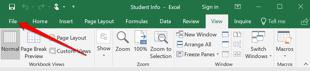
Если ваше приложение Excel является частью вышеупомянутых пакетов Office, вы можете получить доступ к инструменту сравнения электронных таблиц через надстройку «Запрос». Если в вашем приложении Excel нет вкладки «Запрос», вот как ее включить.
- Выбирать Файл в строке меню.
- Выбирать Опции на боковой панели.
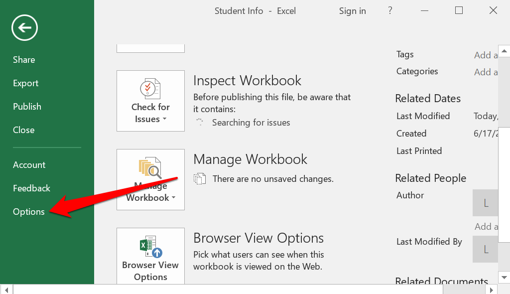
- Выбирать Надстройки на боковой панели выберите Надстройка COM в раскрывающемся меню «Управление» и выберите Идти.
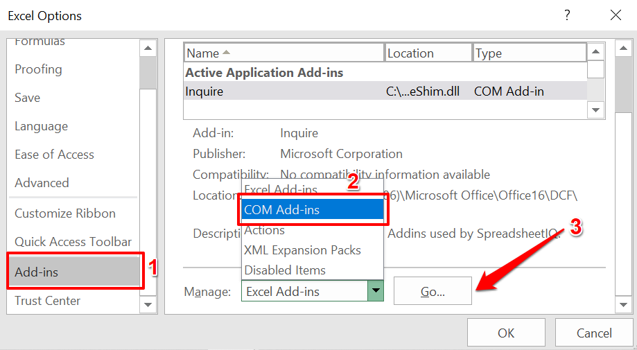
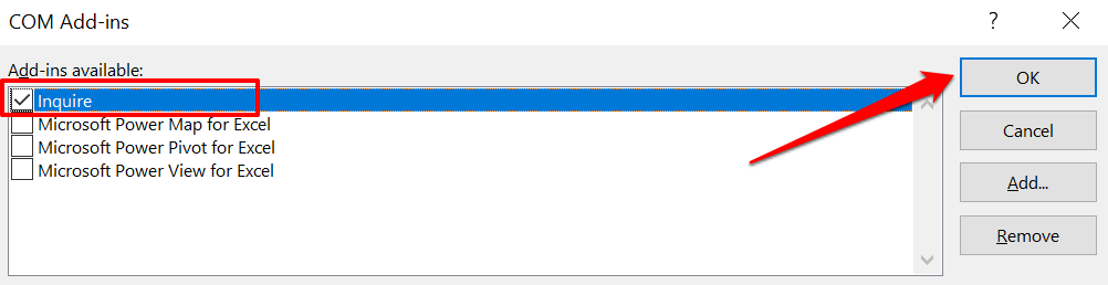
- Проверить Узнать поле и выберите В ПОРЯДКЕ.
Примечание: Если на странице надстроек COM нет флажка «Запросить», значит, ваша версия Excel или Office не поддерживает функцию сравнения электронных таблиц. Или, возможно, администратор вашей организации отключил эту функцию. Установите версии Office с предварительно установленным средством сравнения электронных таблиц или обратитесь к администратору вашей организации.
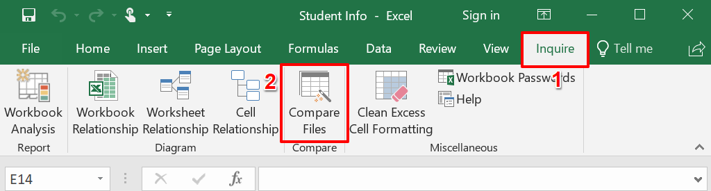
- Откройте оба файла Excel, которые вы хотите сравнить, в отдельном окне, перейдите к Узнать в строке меню и выберите Сравнить файлы.
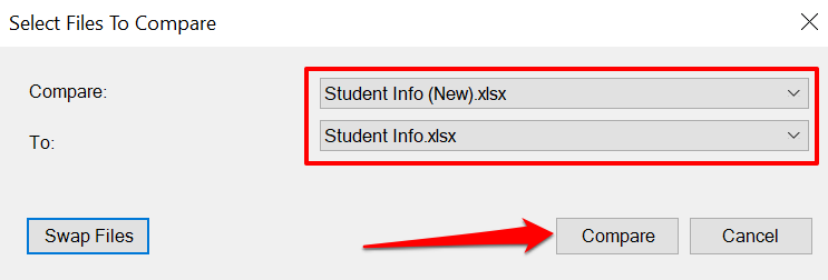
- Excel автоматически добавит первый и второй файлы в диалоговые окна «Сравнить» и «С» соответственно. Выбирать Файлы подкачки для обмена первичными и вторичными файлами или выберите Сравнивать чтобы начать сравнение.
В новом окне будет запущено сравнение электронных таблиц, что подчеркнет любые несоответствия в вашем наборе данных. Обычные ячейки с разными значениями будут выделены зеленым цветом. Ячейки с формулами имеют фиолетовый формат, а ячейки с макросом имеют бирюзовую заливку.
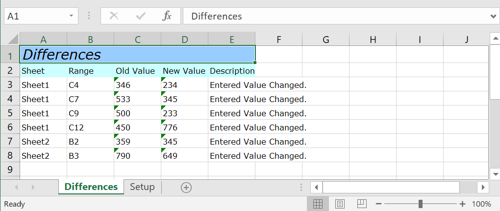
Выбирать Результаты экспорта для создания и сохранения копии результатов на вашем компьютере в виде документа Excel.
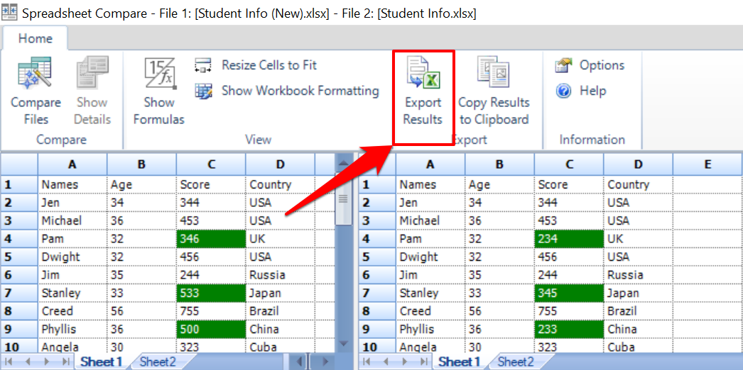
В отчете будут указаны листы и ссылки на ячейки с различными наборами данных, а также точные значения старых и новых данных.
Ты сможешь поделиться отчетом Excel с вашими коллегами, командой или другими людьми, совместно работающими над файлом.
Используйте сравнение электронных таблиц как отдельную программу
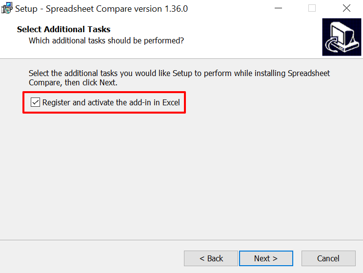
Если в вашей версии Excel или Office нет надстройки для сравнения электронных таблиц, установите автономное программное обеспечение с веб-сайта разработчика. При установке установочного файла обязательно проверьте Зарегистрируйтесь и активируйте надстройку в Excel коробка.
После установки запустите «Сравнение электронных таблиц» и выполните следующие действия, чтобы использовать программу для сравнения документов Excel.
- Выбирать Сравнить файлы во вкладке «Главная».
- Выберите значок папки рядом с диалоговым окном «Сравнить (старые файлы)», чтобы добавить первый документ, который вы хотите сравнить с инструментом. Добавьте второй файл в поле «К (более новые файлы)» и выберите В ПОРЯДКЕ продолжать.
Сравнение электронных таблиц обработает файлы и выделит ячейки с разными значениями зеленым цветом.

Найди отличия
Инструмент сравнения «Просмотр бок о бок» — наиболее подходящий вариант для пользователей Office для дома или студентов. Если вы используете Excel для Microsoft 365 или Office Professional Plus (2013 или 2016), в вашем распоряжении встроенный инструмент «Сравнение электронных таблиц». Но если у вас нет Excel на вашем компьютере, веб-инструменты сравнения Excel сделают вашу работу. Это действительно так просто.
Microsoft Excel has a really cool feature known as “Compare files” that allows you compare two specific files or workbooks and helps you highlighting those changes after the comparison. In this article let us explain how to compare two Excel workbooks.
Why Should You Compare Excel Sheets?
There are many situations you may need to compare two Excel sheets:
- You’re having trouble in finding the updates your colleagues have made in your Excel workbooks.
- When you have two versions of a workbooks like a prior version and a current version, sometimes it required to showcase those changes to your manager in the company.
- You may need to analyze your previous growth. In order to do so, you need to check the data changes in the current file comparison to the prior file.
The problem is even bigger when more than one person is working on the same workbook in Microsoft Excel and hence, there could be more than one versions of the same file. In all such scenario, you have to compare the previous and current workbooks and that will be a good idea before proceeding.
What You Can Compare In Two Excel Workbooks?
The comparison feature actually links to different functions with the help of which it’s able to get us the correct results. There are total 14 areas in which this feature works and more often you are allowed to choose by your preference. You can check or uncheck the needed options. Given below are the areas where this feature works:
- Entered Value
- Calculated Values
- Formulas
- SysGen Formulas
- SysGen Formulas Errors
- Structural
- Names
- SysGen Names
- SysGen Names Error
- Macros
- Data Connection
- Cell Format
- Cell Protection
- Sheet/Workbook Protection
In each of these areas, compare workbook provides you with a really quick method for comparing two of your similar workbooks at the same time.
The first step in comparing two Excel workbooks to have your ‘Inquire’ tab activated in Microsoft Excel. If you’re not having that right now, just follow the steps:
Activating Inquire Tab in Microsoft Excel
- Go to “File > Options” menu. This will open you up a small window of “Excel Options”.
- Now visit the “Add-ins” section. You’ll see active and inactive application add-ins section.
- Under “Inactive Application Add-ins”, click on ‘Inquire’ Add-in and activate.
- Select the “Inquire” add-in and look at the bottom “Manage” options. Select “COM Add-ins” from the dropdown, hit “Go…” button and then press “OK”.
- You’ll have the “Inquire” tab in the ribbon now.

Steps For Comparing Two Excel Workbooks
Let’s say we have two workbooks for comparing their data. We are using here the “Earlier” workbook and “Current” Workbook. In “Earlier” Workbook we have done some changes and saved it as new one name “Current” Workbook. Earlier Workbook has old data and “Current” has some changed data.
- Step 1: We have our Earlier workbook like this:

- Step 2: Here is our Current Workbook which has some changed data as you can see.

- Step 3: Now, go to any of the workbooks. Click on “Inquire” tab and then under “Compare” section, click on “Compare Files”.

- Step 4: You’ll see a compare window asking you to choose compare file and to which file you want to compare it with. In our case, the Earlier file goes with “Compare” option and Current file goes with “To” option. You can swap files easily by clicking on the “Swap Files” button.

- Step 5: Click on “Compare” button and you will see a new window showing the results of the comparison. In our case, it is the status “Out of stock” in Earlier file which is changed to “In stock” in the Current file. You can also see the detailed description given below like “Entered Value Changed”.

When you have more changes, Excel will group the changes into different categories and list down all changes between two compared files.
Related Articles:
- How to use VLOOKUP and HLOOKUP in Excel?
- Shortcuts to change cell format in Excel quickly
- Show table header in multiple pages in Excel and Word
- How to use mail merge in Microsoft Word?
- Change page orientation in Microsoft Word
What You Can’t Compare?
There are some areas where this feature won’t work directly. This feature, first of all, finds all the sheets in the workbook that have the same name with identical names. It compares cell by cell value in each sheet. VBA projects, cell formats, comments, charts, objects are not compared in this feature.
This feature works with only two workbooks not more than that. As you have seen above, in comparison windows, you are able to add 2 workbooks only. So, this could be a limitation of this feature. If any workbook is protected, this feature will not allow that file to be compared. You need to unprotect it first then you can use it for comparison.
Conclusion
In the above guide, we have shared that what you can compare, how to compare, and what you cannot compare in Microsoft Excel’s comparison feature. Now, make sure that you compare the similar files to get the correct result. You will not be able to use an object, VBA project and more stuff like that as explained above. You can only be allowed to compare two workbooks at a once.