
Excel for Microsoft 365 Excel for Microsoft 365 for Mac Excel 2021 Excel 2021 for Mac Excel 2019 Excel 2019 for Mac Excel 2016 Excel 2016 for Mac Excel 2013 Office for business Excel 2010 Excel 2007 More…Less
You can use the following methods to compare data in two Microsoft Excel worksheet columns and find duplicate entries.
Method 1: Use a worksheet formula
-
Start Excel.
-
In a new worksheet, enter the following data as an example (leave column B empty):
A
B
C
1
1
3
2
2
5
3
3
8
4
4
2
5
5
0
-
Type the following formula in cell B1:
=IF(ISERROR(MATCH(A1,$C$1:$C$5,0)),»»,A1)
-
Select cell B1 to B5.
-
In Excel 2007 and later versions of Excel, select Fill in the Editing group, and then select Down.
The duplicate numbers are displayed in column B, as in the following example:
A
B
C
1
1
3
2
2
2
5
3
3
3
8
4
4
2
5
5
5
0
Method 2: Use a Visual Basic macro
Warning: Microsoft provides programming examples for illustration only, without warranty either expressed or implied. This includes, but is not limited to, the implied warranties of merchantability or fitness for a particular purpose. This article assumes that you are familiar with the programming language that is being demonstrated and with the tools that are used to create and to debug procedures. Microsoft support engineers can help explain the functionality of a particular procedure. However, they will not modify these examples to provide added functionality or construct procedures to meet your specific requirements.
To use a Visual Basic macro to compare the data in two columns, use the steps in the following example:
-
Start Excel.
-
Press ALT+F11 to start the Visual Basic editor.
-
On the Insert menu, select Module.
-
Enter the following code in a module sheet:
Sub Find_Matches() Dim CompareRange As Variant, x As Variant, y As Variant ' Set CompareRange equal to the range to which you will ' compare the selection. Set CompareRange = Range("C1:C5") ' NOTE: If the compare range is located on another workbook ' or worksheet, use the following syntax. ' Set CompareRange = Workbooks("Book2"). _ ' Worksheets("Sheet2").Range("C1:C5") ' ' Loop through each cell in the selection and compare it to ' each cell in CompareRange. For Each x In Selection For Each y In CompareRange If x = y Then x.Offset(0, 1) = x Next y Next x End Sub -
Press ALT+F11 to return to Excel.
-
Enter the following data as an example (leave column B empty):
A
B
C
1
1
3
2
2
5
3
3
8
4
4
2
5
5
0
-
-
Select cell A1 to A5.
-
In Excel 2007 and later versions of Excel, select the Developer tab, and then select Macros in the Code group.
Note: If you don’t see the Developer tab, you may have to turn it on. To do this, select File > Options > Customize Ribbon, and then select the Developer tab in the customization box on the right-side.
-
Click Find_Matches, and then click Run.
The duplicate numbers are displayed in column B. The matching numbers will be put next to the first column, as illustrated here:
A
B
C
1
1
3
2
2
2
5
3
3
3
8
4
4
2
5
5
5
0
Need more help?
Want more options?
Explore subscription benefits, browse training courses, learn how to secure your device, and more.
Communities help you ask and answer questions, give feedback, and hear from experts with rich knowledge.
Watch Video – Compare two Columns in Excel for matches and differences
The one query that I get a lot is – ‘how to compare two columns in Excel?’.
This can be done in many different ways, and the method to use will depend on the data structure and what the user wants from it.
For example, you may want to compare two columns and find or highlight all the matching data points (that are in both the columns), or only the differences (where a data point is in one column and not in the other), etc.
Since I get asked about this so much, I decided to write this massive tutorial with an intent to cover most (if not all) possible scenarios.
If you find this useful, do pass it on to other Excel users.
Note that the techniques to compare columns shown in this tutorial are not the only ones.
Based on your dataset, you may need to change or adjust the method. However, the basic principles would remain the same.
If you think there is something that can be added to this tutorial, let me know in the comments section
Compare Two Columns For Exact Row Match
This one is the simplest form of comparison. In this case, you need to do a row by row comparison and identify which rows have the same data and which ones does not.
Example: Compare Cells in the Same Row
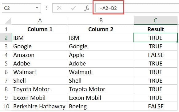
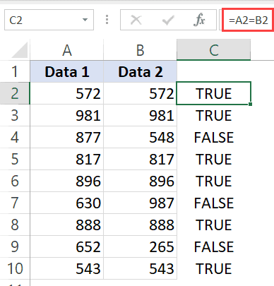
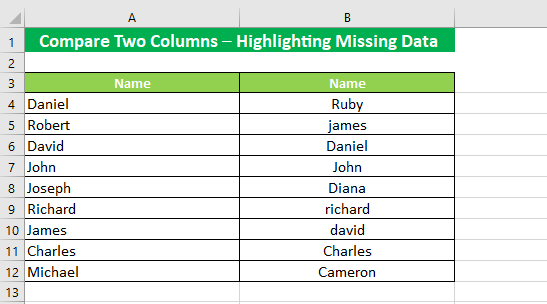
Below is a data set where I need to check whether the name in column A is the same in column B or not.
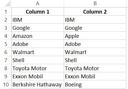
If there is a match, I need the result as “TRUE”, and if doesn’t match, then I need the result as “FALSE”.
The below formula would do this:
=A2=B2
Example: Compare Cells in the Same Row (using IF formula)
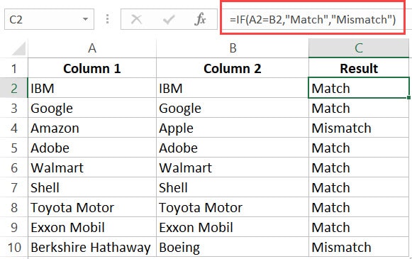
If you want to get a more descriptive result, you can use a simple IF formula to return “Match” when the names are the same and “Mismatch” when the names are different.
=IF(A2=B2,"Match","Mismatch")
Note: In case you want to make the comparison case sensitive, use the following IF formula:
=IF(EXACT(A2,B2),"Match","Mismatch")
With the above formula, ‘IBM’ and ‘ibm’ would be considered two different names and the above formula would return ‘Mismatch’.
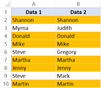
Example: Highlight Rows with Matching Data
If you want to highlight the rows that have matching data (instead of getting the result in a separate column), you can do that by using Conditional Formatting.
Here are the steps to do this:
- Select the entire dataset.
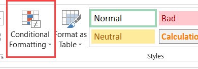
- Click the ‘Home’ tab.

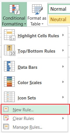
- In the Styles group, click on the ‘Conditional Formatting’ option.

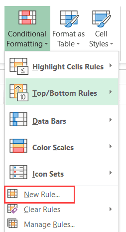
- From the drop-down, click on ‘New Rule’.

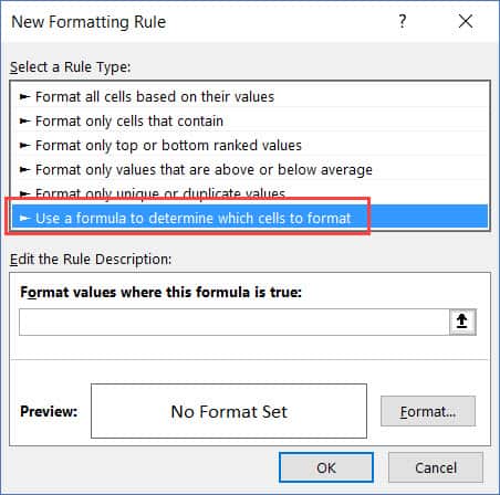
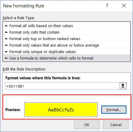
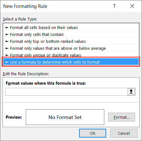
- In the ‘New Formatting Rule’ dialog box, click on the ‘Use a formula to determine which cells to format’.

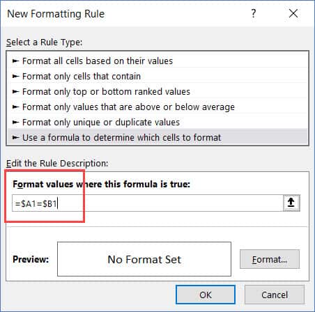
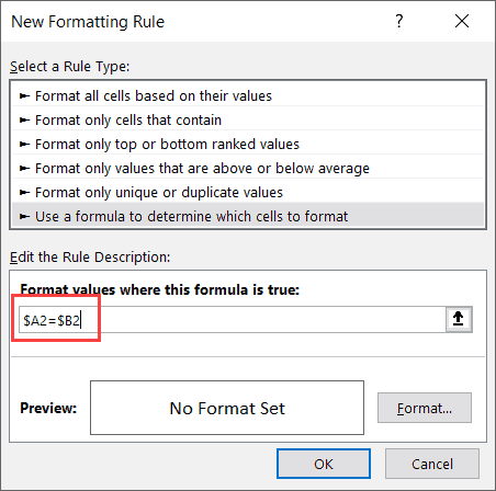
- In the formula field, enter the formula: =$A1=$B1
- Click the Format button and specify the format you want to apply to the matching cells.
- Click OK.
This will highlight all the cells where the names are the same in each row.
Compare Two Columns and Highlight Matches
If you want to compare two columns and highlight matching data, you can use the duplicate functionality in conditional formatting.
Note that this is different than what we have seen when comparing each row. In this case, we will not be doing a row by row comparison.
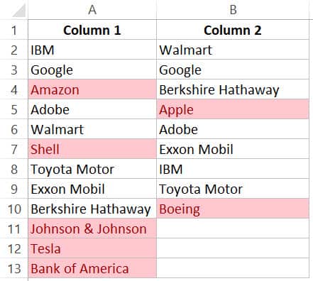
Example: Compare Two Columns and Highlight Matching Data
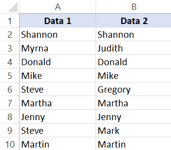
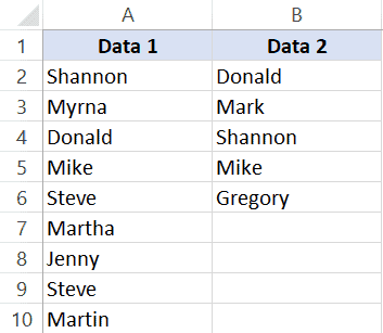
Often, you’ll get datasets where there are matches, but these may not be in the same row.
Something as shown below:
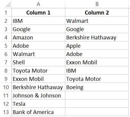
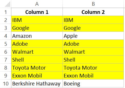
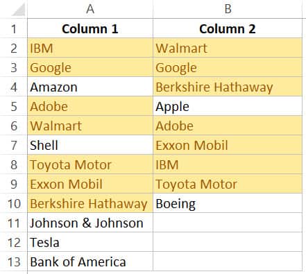
Note that the list in column A is bigger than the one in B. Also some names are there in both the lists, but not in the same row (such as IBM, Adobe, Walmart).
If you want to highlight all the matching company names, you can do that using conditional formatting.
Here are the steps to do this:
- Select the entire data set.
- Click the Home tab.
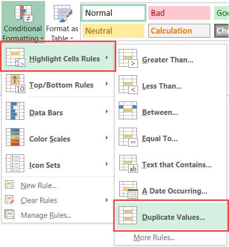
- In the Styles group, click on the ‘Conditional Formatting’ option.
- Hover the cursor on the Highlight Cell Rules option.
- Click on Duplicate Values.

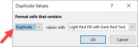
- In the Duplicate Values dialog box, make sure ‘Duplicate’ is selected.

- Specify the formatting.

- Click OK.
The above steps would give you the result as shown below.
Note: Conditional Formatting duplicate rule is not case sensitive. So ‘Apple’ and ‘apple’ are considered the same and would be highlighted as duplicates.
Example: Compare Two Columns and Highlight Mismatched Data
In case you want to highlight the names which are present in one list and not the other, you can use the conditional formatting for this too.
- Select the entire data set.
- Click the Home tab.
- In the Styles group, click on the ‘Conditional Formatting’ option.
- Hover the cursor on the Highlight Cell Rules option.
- Click on Duplicate Values.
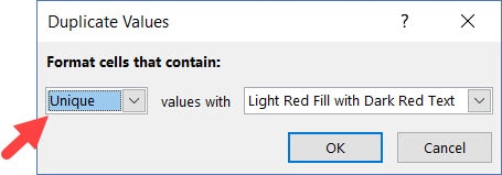
- In the Duplicate Values dialog box, make sure ‘Unique’ is selected.

- Specify the formatting.
- Click OK.
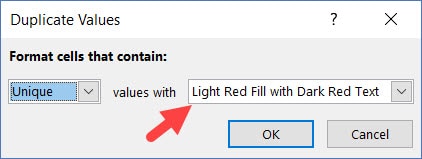
This will give you the result as shown below. It highlights all the cells that have a name that is not present on the other list.
Compare Two Columns and Find Missing Data Points
If you want to identify whether a data point from one list is present in the other list, you need to use the lookup formulas.
Suppose you have a dataset as shown below and you want to identify companies that are present in column A but not in Column B,
To do this, I can use the following VLOOKUP formula.
=ISERROR(VLOOKUP(A2,$B$2:$B$10,1,0))
This formula uses the VLOOKUP function to check whether a company name in A is present in column B or not. If it is present, it will return that name from column B, else it will return a #N/A error.
These names which return the #N/A error are the ones that are missing in Column B.
ISERROR function would return TRUE if there is the VLOOKUP result is an error and FALSE if it isn’t an error.
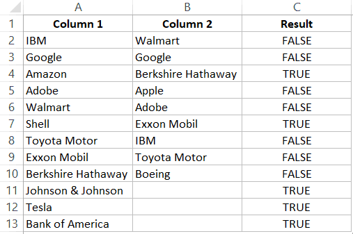
If you want to get a list of all the names where there is no match, you can filter the result column to get all cells with TRUE.
You can also use the MATCH function to do the same;
=NOT(ISNUMBER(MATCH(A2,$B$2:$B$10,0)))
Note: Personally, I prefer using the Match function (or the combination of INDEX/MATCH) instead of VLOOKUP. I find it more flexible and powerful. You can read the difference between Vlookup and Index/Match here.
Compare Two Columns and Pull the Matching Data
If you have two datasets and you want to compare items in one list to the other and fetch the matching data point, you need to use the lookup formulas.
Example: Pull the Matching Data (Exact)
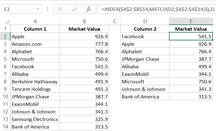
For example, in the below list, I want to fetch the market valuation value for column 2. To do this, I need to look up that value in column 1 and then fetch the corresponding market valuation value.
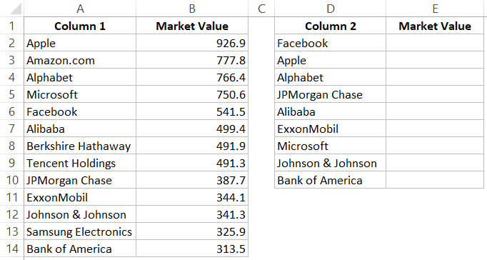
Below is the formula that will do this:
=VLOOKUP(D2,$A$2:$B$14,2,0)
or
=INDEX($A$2:$B$14,MATCH(D2,$A$2:$A$14,0),2)
Example: Pull the Matching Data (Partial)
In case you get a dataset where there is a minor difference in the names in the two columns, using the above-shown lookup formulas is not going to work.
These lookup formulas need an exact match to give the right result. There is an approximate match option in VLOOKUP or MATCH function, but that can’t be used here.
Suppose you have the data set as shown below. Note that there are names that are not complete in Column 2 (such as JPMorgan instead of JPMorgan Chase and Exxon instead of ExxonMobil).
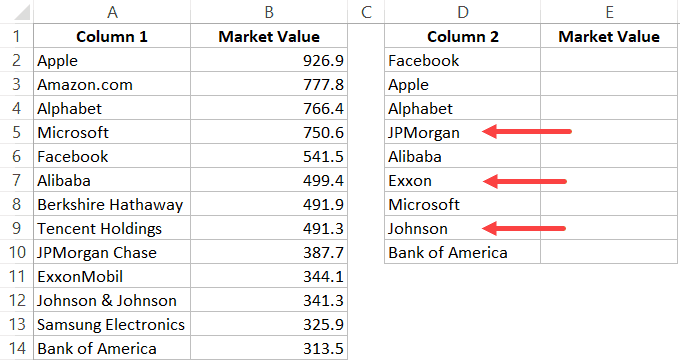
In such a case, you can use a partial lookup by using wildcard characters.
The following formula will give is the right result in this case:
=VLOOKUP("*"&D2&"*",$A$2:$B$14,2,0)
or
=INDEX($A$2:$B$14,MATCH("*"&D2&"*",$A$2:$A$14,0),2)
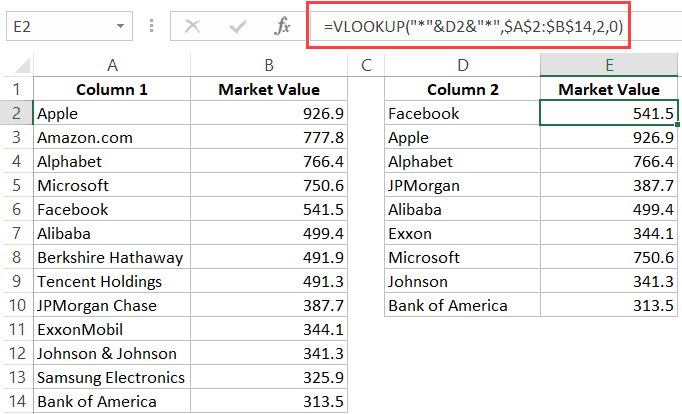
In the above example, the asterisk (*) is a wildcard character that can represent any number of characters. When the lookup value is flanked with it on both sides, any value in Column 1 which contains the lookup value in Column 2 would be considered as a match.
For example, *Exxon* would be a match for ExxonMobil (as * can represent any number of characters).
You May Also Like the Following Excel Tips & Tutorials:
- How to Compare Two Excel Sheets (for differences)
- How to Highlight Blank Cells in Excel.
- How to Compare Text in Excel (Easy Formulas)
- Highlight EVERY Other ROW in Excel.
- Excel Advanced Filter: A Complete Guide with Examples.
- Highlight Rows Based on a Cell Value in Excel
- How to Compare Dates in Excel (Greater/Less Than, Mismatches)
When you’re working with data in Excel, sooner or later you will have to compare data. This could be comparing two columns or even data in different sheets/workbooks.
In this Excel tutorial, I will show you different methods to compare two columns in Excel and look for matches or differences.
There are multiple ways to do this in Excel and in this tutorial I will show you some of these (such as comparing using VLOOKUP formula or IF formula or Conditional formatting).
So let’s get started!
Compare Two Columns (Side by Side)
This is the most basic type of comparison where you need to compare a cell in one column with the cell in the same row in another column.
Suppose you have a dataset as shown below and you simply want to check whether the value in column A in a specific cell is the same (or different) when compared with the value in the adjacent cell.
Of course, you can do this when you have a small dataset when you have a large one, you can use a simple comparison formula to get this done. And remember, there is always a chance of human error when you do this manually.
So let me show you a couple of easy ways to do this.
Compare Side by Side Using the Equal to Sign Operator
Suppose you have the below dataset and you want to know what rows have the matching data and what rows have different data.
Below is a simple formula to compare two columns (side by side):
=A2=B2
The above formula will give you a TRUE if both the values are the same and FALSE in case they are not.
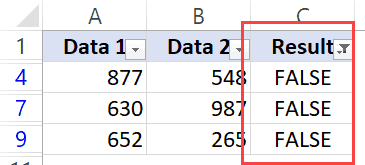
Now, if you need to know all the values that match, simply apply a filter and only show all the TRUE values. And if you want to know all the values that are different, filter all the values that are FALSE (as shown below):
When using this method to do column comparison in Excel, it’s always best to check that your data does not have any leading or trailing spaces. If these are present, despite having the same value, Excel will show them as different. Here is a great guide on how to remove leading and trailing spaces in Excel.
Compare Side by Side Using the IF Function
Another method that you can use to compare two columns can be by using the IF function.
This is similar to the method above where we used the equal to (=) operator, with one added advantage. When using the IF function, you can choose the value you want to get when there are matches or differences.
For example, if there is a match, you can get the text “Match” or can get a value such as 1. Similarly, when there is a mismatch, you can program the formula to give you the text “Mismatch” or give you a 0 or blank cell.
Below is the IF formula that returns ‘Match’ when the two cells have the cell value and ‘Not a Match’ when the value is different.
=IF(A2=B2,"Match","Not a Match")
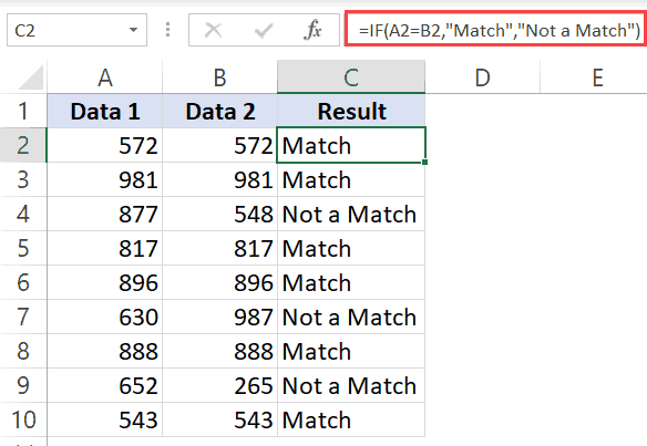
The above formula uses the same condition to check whether the two cells (in the same row) have matching data or not (A2=B2). But since we are using the IF function, we can ask it to return a specific text in case the condition is True or False.
Once you have the formula results in a separate column, you can quickly filter the data and get rows that have the matching data or rows with mismatched data.
Also read: Does Not Equal Operator in Excel (Examples)
Highlight Rows with Matching Data (or Different Data)
Another great way to quickly check the rows that have matching data (or have different data), is to highlight these rows using conditional formatting.
You can do both – highlight rows that have the same value in a row as well as the case when the value is different.
Suppose you have a dataset as shown below and you want to highlight all the rows where the name is the same.
Below are the steps to use conditional formatting to highlight rows with matching data:
- Select the entire dataset (except the headers)
- Click the Home tab

- In the Styles group, click on Conditional Formatting

- In the options that show up, click on ‘New Rule’

- In the ‘New Formatting Rule’ dialog box, click on the option -”Use a formula to determine which cells to format’
- In the ‘Format values where this formula is true’ field, enter the formula: =$A2=$B2
- Click on the Format button
- Click on the ‘Fill’ tab and select the color in which you want to highlight the rows with the same value in both columns

- Click OK

The above steps would instantly highlight the rows where the name is the same in both columns A and B (in the same row). And in the case where the name is different, those rows will not be highlighted.
In case you want to compare two columns and highlight rows where the names are different, use the below formula in the conditional formatting dialog box (in step 6).
=$A2<>$B2
How does this work?
When we use conditional formatting with a formula, it only highlights those cells where the formula is true.
When we use $A2=$B2, it will check each cell (in both columns) and see whether the value in a row in column A is equal to the one in column B or not.
In case it’s an exact match, it will highlight it in the specified color, and in case it doesn’t match, it will not.
The best part about conditional formatting is that it doesn’t require you to use a formula in a separate column. Also, when you apply the rule on a dataset, it remains dynamic. This means that if you change any name in the dataset, conditional formatting will accordingly adjust.
Compare Two Columns Using VLOOKUP (Find Matching/Different Data)
In the above examples, I showed you how to compare two columns (or lists) when we are just comparing side by side cells.
In reality, this is rarely going to be the case.
In most cases, you will have two columns with data and you would have to find out whether a data point in one column exists in the other column or not.
In such cases, you can’t use a simple equal-to sign or even an IF function.
You need something more powerful…
… something that’s right up VLOOKUP’s alley!
Let me show you two examples where we compare two columns in Excel using the VLOOKUP function to find matches and differences.
Compare Two Columns Using VLOOKUP and Find Matches
Suppose we have a dataset as shown below where we have some names in columns A and B.
If you have to find out what are the names that are in column B that are also in column A, you can use the below VLOOKUP formula:
=IFERROR(VLOOKUP(B2,$A$2:$A$10,1,0),"No Match")
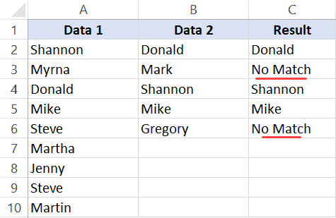
The above formula compares the two columns (A and B) and gives you the name in case the name is in column B as well A, and it returns “No Match” in case the name is in Column B and not in Column A.
By default, the VLOOKUP function will return a #N/A error in case it doesn’t find an exact match. So to avoid getting the error, I have wrapped the VLOOKUP function in the IFERROR function, so that it gives “No Match” when the name is not available in column A.
You can also do the other way round comparison – to check whether the name is in Column A as well as Column B. The below formula would do that:
=IFERROR(VLOOKUP(A2,$B$2:$B$6,1,0),"No Match")
Compare Two Columns Using VLOOKUP and Find Differences (Missing Data Points)
While in the above example, we checked whether the data in one column was there in another column or not.
You can also use the same concept to compare two columns using the VLOOKUP function and find missing data.
Suppose we have a dataset as shown below where we have some names in columns A and B.
If you have to find out what are the names that are in column B that not there in column A, you can use the below VLOOKUP formula:
=IF(ISERROR(VLOOKUP(B2,$A$2:$A$10,1,0)),"Not Available","Available")
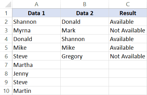
The above formula checks the name in column B against all the names in Column A. In case it finds an exact match, it would return that name, and in case it doesn’t find and exact match, it will return the #N/A error.
Since I am interested in finding the missing names that are there is column B and not in column A, I need to know the names that return the #N/A error.
This is why I have wrapped the VLOOKUP function in the IF and ISERROR functions. This whole formula gives the value – “Not Available” when the name is missing in Column A, and “Available” when it’s present.
To know all the names that are missing, you can filter the result column based on the “Not Available” value.
You can also use the below MATCH function to get the same result:
=IF(ISNUMBER(MATCH(B2,$A$2:$A$10,0)),"Available","Not Available")
Common Queries when Comparing Two Columns
Below are some common queries I usually get when people are trying to compare data in two columns in Excel.
Q1. How to compare multiple columns in Excel in the same row for matches? Count the total duplicates also.
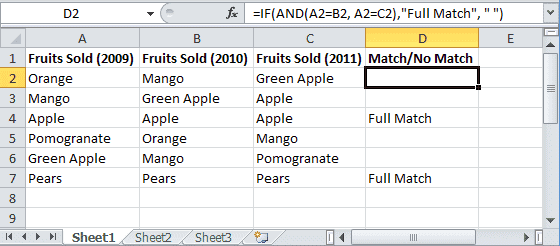
Ans. We have given the procedure to compare two columns in excel for the same row above. But if you want to compare multiple columns in excel for the same row then see the example
=IF(AND(A2=B2, A2=C2),"Full Match", "")
Here we have compared data of column A, column B, and column C. After this, I have applied the above formula in column D and get the result.
Now to count the duplicates, you need to use the Countif function.
=IF(COUNTIF($A2:$E2, $A2)=5, "Full Match", "")
Q2. Which operator do you use for matches and differences?
Ans. Below are the operators to use:
- To find matches, use the equal to sign (=)
- To find differences (mismatches), use the not-equal-to sign (<>)
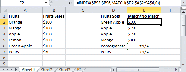
Q3. How to compare two different tables and pull matching data?
Ans. For this, you can use the VLOOKUP function or INDEX & MATCH function. To understand this thing in a better way we will take an example.
Here we will take two tables and now want to do pull matching data. In the first table, you have a dataset and in the second table, take the list of fruits and then use pull matching data in another column. For pull matching, use the formula
=INDEX($B$2:$B$6,MATCH($D2,$A$2:$A$6,0))
Q4. How to remove duplicates in Excel?
Ans. To remove duplicate data you need to first find the duplicate values.
To find the duplicate, you can use various methods like conditional formatting, Vlookup, If Statement, and many more. Excel also has an in-built tool where you can just select the data, and remove the duplicates from a column or even multiple columns
Q5. I can see that there is a matching value in both columns. However, the formulas you have shared above are not considering these as exact matches. Why?
Ans: Excel considers something an exact match when each and every character of one cell is equal to the other. There is a high chance that in your dataset there are leading or trailing spaces.
Although these spaces may still make the values seem equal to a naked eye, for Excel these are different. If you have such a dataset, it’s best to get rid of these spaces (you can use Excel functions such as TRIM for this).
Q7. How to compare two columns that give the result as TRUE when all first columns’ integer values are not less than the second column’s integer values. To solve this problem, I do not require conditional formatting, Vlookup function, If Statement, and any other formulas. I need the formula to solve this problem.
Ans. You can use the array formula for solving this problem.
The syntax is {=AND(H6:H12>I6:I12)}. This will give you “True” as a result whenever the value of Column H is greater than the value in column I else “False” will be the result.
You may also like the following Excel tutorials:
- Compare Two Columns in Excel (for matches and differences)
- How to Remove Blank Columns in Excel? (Formula + VBA)
- How to Hide Columns Based On Cell Value in Excel
- How to Split One Column into Multiple Columns in Excel
- How to Select Alternate Columns in Excel (or every Nth Column)
- How to Paste in a Filtered Column Skipping the Hidden Cells
- Best Excel Books (that will make you an Excel Pro)
- How to Flip Data in Excel (Columns, Rows, Tables)?
- Find the Closest Match in Excel (Nearest Value)
- How to Compare Two Cells in Excel?
- VLOOKUP Not Working – 7 Possible Reasons + How to Fix!
Two columns in excel are compared when their entries are studied for similarities and differences. The similarities are the data values that exist in the same row of both the compared columns. In contrast, the differences are those values that exist in only one of these columns.
For example, for a specific month, a table displays the following information:
- Column A lists the names of the employees who took three consecutive leaves.
- Column B lists the names of the employees who took two consecutive leaves.
Since the data pertains to the same organization, there can be a similarity or a difference within the given set of values. The same is explained as follows:
- A similarity or a match (column A is equal to column B) implies employees who took both three and two continuous leaves.
- A difference (column A is not equal to column B) implies employees who took either three or two continuous leaves.
It is difficult to scan through the data to track the matches and the differences manually. Hence, there are techniques which can be followed to compare 2 columns of an excel worksheet.
Table of contents
- Compare two Columns in Excel
- How to Compare two Columns in Excel? (Top 4 Methods)
- #1 – Compare Using Simple Formulae
- #2 – Compare 2 Columns Using the IF Formula
- #3 – Compare Using the EXACT Formula
- #4 – Compare 2 Excel Columns Using Conditional Formatting
- The Properties of the Comparison Methods
- Frequently Asked Questions
- Recommended Articles
- How to Compare two Columns in Excel? (Top 4 Methods)
How to Compare two Columns in Excel? (Top 4 Methods)
The top four methods to compare 2 columns are listed as follows:
- Method #1–Compare using simple formulae
- Method #2–Compare using the IF formula
- Method #3–Compare using the EXACT formula
- Method #4–Compare using conditional formatting
Let us understand these methods with the help of examples.
You can download this Compare Two Columns Excel Template here – Compare Two Columns Excel Template
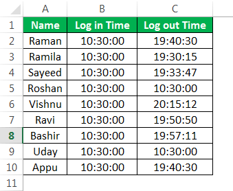
#1 – Compare Using Simple Formulae
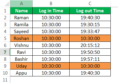
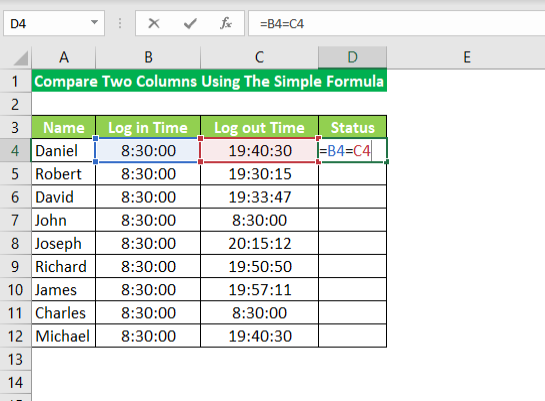
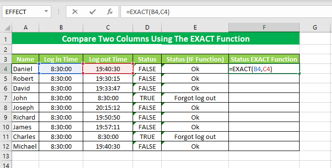
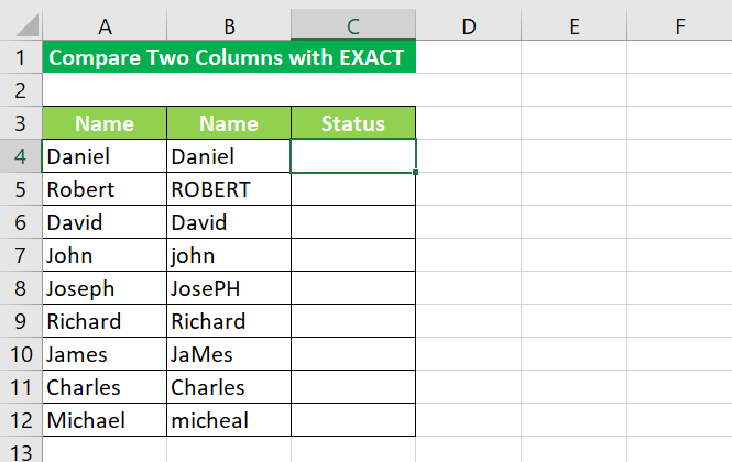
The following table shows the names of the employees of an organization in column A. Columns B and C display their log-in and the log-out times respectively.
We want to compare two excel columns B and C to find out the employees who forgot to logout from the office. The official timings are 10:30 a.m.-7:30 p.m. Use the formula method for comparison.
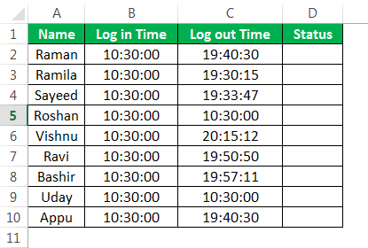
For the given data, if the log-in time is equal to the log-out time, we assume that the employee has forgotten to logout.
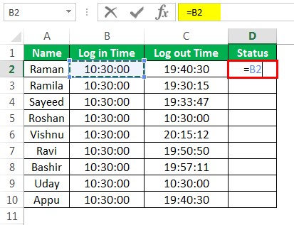
The steps to compare two columns in excel with the help of the comparison operator “equal to” (=) are listed as follows:
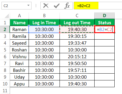
- In cell D2, enter the symbol “=” followed by selecting the cell B2.

- Enter the symbol “=” again, followed by selecting the cell C2.

- Press the “Enter” key. It returns “false.” This implies that the value in cell B2 is not equal to that of cell C2.

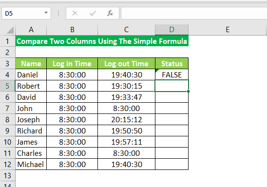
- Drag or copy-paste the formula to the remaining cells. The output is either “true” or “false,” as shown in the following image.
If the value in column B is equal to that of column C, the result is “true,” else “false.” The cells D5 and D9 show the output “true.”
Hence, Roshan and Uday forgot to logout from the office.

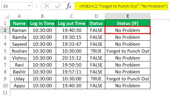
#2 – Compare 2 Columns Using the IF Formula
Working on the data of example #1, we want the following results:
- “Forgot to punch out,” if the employee forgets to logout
- “No problem,” if the employee logs out
Use the IF functionIF function in Excel evaluates whether a given condition is met and returns a value depending on whether the result is “true” or “false”. It is a conditional function of Excel, which returns the result based on the fulfillment or non-fulfillment of the given criteria.
read more to compare the columns B and C.
We apply the following formula.
“=IF(B2=C2,“Forgot to Punch Out”,“No Problem”)”
If the value in column B is equal to that of column C, the result is “true,” otherwise “false.” For every “true” value, the formula returns “forgot to punch out.” Likewise, it returns “no problem” for every “false” value.
The output is shown in column E of the following image.
Hence, Roshan and Uday are the only two employees who have forgotten to logout from the office.
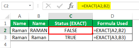
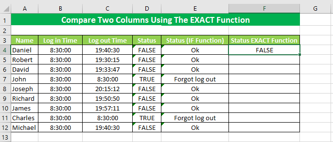
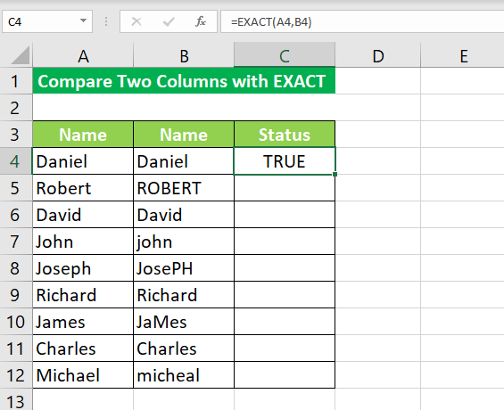
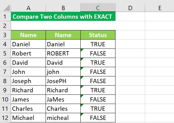
#3 – Compare Using the EXACT Formula
Working on the data of example #1, we want to compare the two excel columns B and C with the help of the EXACT functionThe exact function is a logical function in excel used to compare two strings or data with each other, and it gives us the result whether the both data are an exact match or not. This function is a logical function, so it provides true or false as a result.read more.
We apply the following formula.
“=EXACT(B2,C2)”
If the value in column B is equal to that of column C, the formula returns “true,” otherwise “false.” The output is shown in column F of the following image.
Hence, the entries of columns B and C are identical for Roshan and Uday.
Note: The EXACT function is case-sensitive.

We have written the name “Raman” in columns A and B with different casing. We apply the following formula.
“=EXACT(A2,B2)”
The formula returns “false” when the casing of cell A2 is different from that of cell B2. Likewise, it returns “true” if the casing in columns A and B is the same.
The output is shown in column C of the following image.
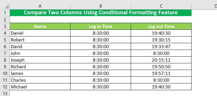
#4 – Compare 2 Excel Columns Using Conditional Formatting
Working on the data of example #1, we want to highlight those entries that are identical in columns B and C. Use the conditional formattingConditional formatting is a technique in Excel that allows us to format cells in a worksheet based on certain conditions. It can be found in the styles section of the Home tab.read more feature.
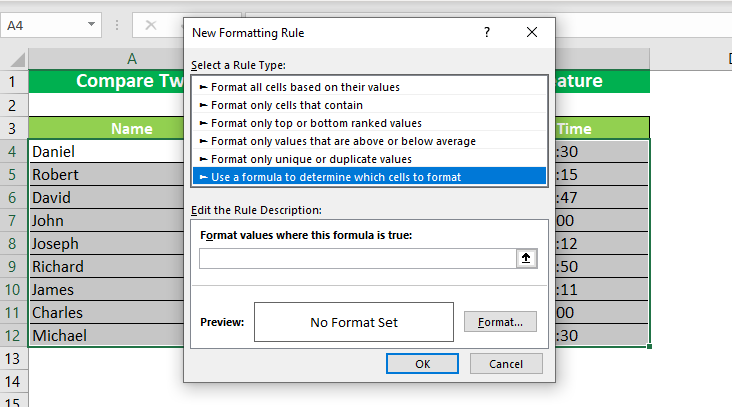
Step 1: Select the entire data. In the Home tab, click the “conditional formatting” drop-down under the “styles” section. Select “new rule.”
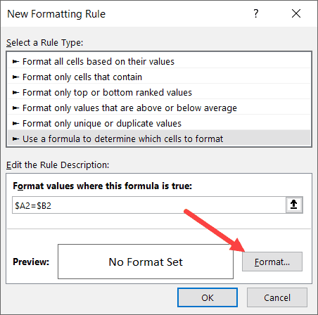
Step 2: The “new formatting rule” window appears. Under “select a rule type,” choose the option “use a formula to determine which cells to format.”
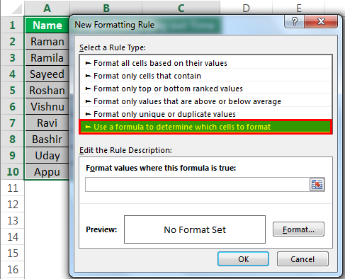
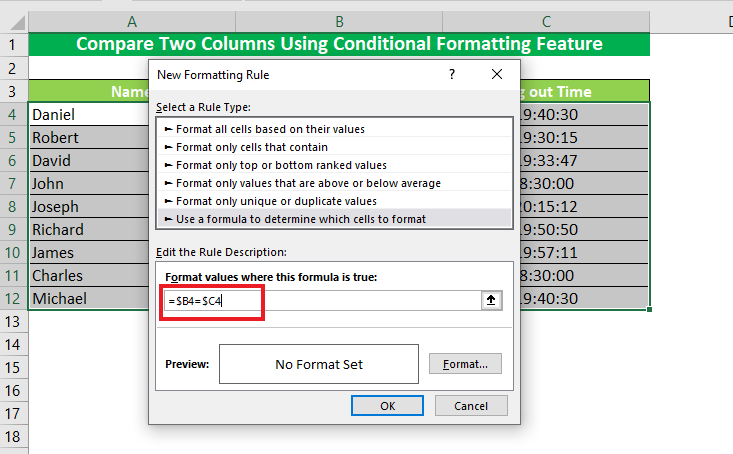
Step 3: Enter the formula “$B2=$C2” under “edit the rule description.”
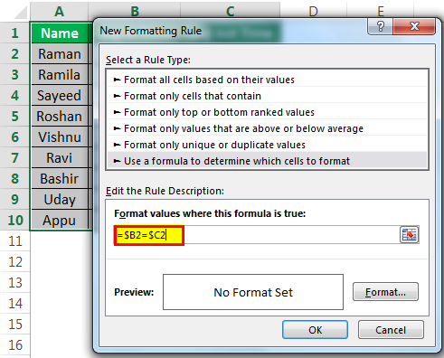
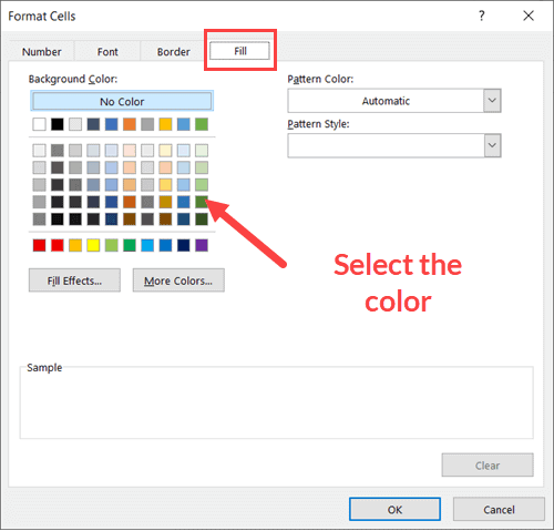
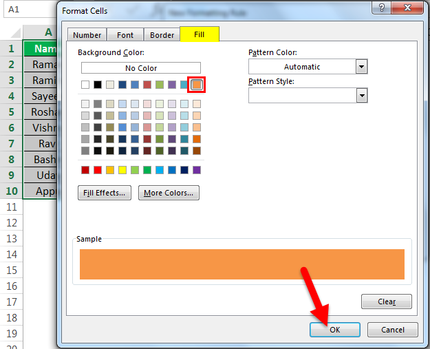
Step 4: Click “format.” In the “format cells” window, select the color to highlight the identical entries. Click “Ok.” Click “Ok” again in the “new formatting rule” window.
Step 5: The matches of columns B and C are highlighted, as shown in the following image.
Hence, the entries of columns B and C are identical for Roshan and Uday.
The Properties of the Comparison Methods
The features of the comparison methods discussed are listed as follows:
- The outcomes of the IF function can be modified according to the requirement of the user.
- The EXACT function returns “false” for two same values having different casing.
- The simplest technique to compare two excel columns is by using the comparison operator “equal to” (method #1).
Note: The comparison method to be used depends on the data structure and the kind of output required.
Frequently Asked Questions
1. What does it mean to compare two columns and how is it done in Excel?
The comparison of two data columns helps find the similarities and the differences. In case of similarity, a value exists in the same row of both the columns. In contrast, a difference is a deviation of one value from the other.
To compare two excel columns, the easiest approach is listed as follows:
a. Enter the following formula.
“=cell1=cell2”
The “cell1” is a cell containing a data value in the first column. The “cell2” is a cell containing a data value in the second column. Both “cell1” and “cell2” are in the same row.
b. Press the “Enter” key.
The formula returns “true” or “false” depending on whether the value exists in both the compared columns or not.
2. How to highlight the different values of two columns without using the formula in Excel?
Let us compare the following 2 columns consisting of names in the mentioned sequence:
• Column A contains Jack, Adam, Elizabeth, Betty, and Veronica.
• Column B contains Robert, Peter, Elizabeth, Henry, and Veronica.
The steps to highlight the different values without using the formula are listed as follows:
a. Select columns A and B.
b. In the Home tab, click “find and select” drop-down under the “editing” group. Choose “go to special.”
c. In the “go to special” window, select “row differences.” Click “Ok.”
The names Robert, Peter, and Henry of column B are highlighted. These cells can be colored using the “fill color” property of Excel.
3. How to compare multiple columns in Excel?
Let us compare the following columns consisting of numbers in the mentioned sequence:
• Column A contains 3, 49, 20, 22, and 86 in the range A1:A5.
• Column B contains 29, 49, 38, 21, and 86 in the range B1:B5.
• Column C contains 12, 49, 56, 24, and 86 in the range C1:C5.
The steps to compare columns A, B, and C are stated as follows:
a. Enter the following formula in cell D1. “IF(COUNTIF($A1:$C5,$A1)=3,“full match”,“”)”
b. Press the “Enter” key.
c. Drag or copy-paste the formula to the remaining cells.
Since we are comparing three excel columns, we enter the number 3 in the formula. The formula returns “full match” in cells D2 and D5. It returns an empty string in the cells D1, D3, and D4.
Hence, the numbers 49 and 86 appear in the respective rows 2 and 5 of all the three columns.
Recommended Articles
This has been a guide to compare two columns in Excel. Here we discussed the top 4 methods to compare 2 columns in Excel, 1) the operator “equal to”, 2) IF function, 3) EXACT formula, and 4) conditional formatting. We also went through some practical examples. You can download the Excel template from the website. For more on Excel, take a look at the following articles-
- Freeze Columns in ExcelFreezing columns in excel fixes or locks them so that they remain visible while scrolling through the database. A frozen column does not move with the movement of the remaining columns.read more
- Excel Rows to ColumnsRows can be transposed to columns by using paste special method and the data can be linked to the original data by simply selecting ‘Paste Link’ form the paste special dialog box. It could also be done by using INDIRECT formula and ADDRESS functions.read more
- Count Only Unique Values in ExcelIn Excel, there are two ways to count values: 1) using the Sum and Countif function, and 2) using the SUMPRODUCT and Countif function.read more
- Advanced Filter in ExcelThe advanced filter is different from the auto filter in Excel. This feature is not like a button that one can use with a single click of the mouse. To use an advanced filter, we have to define criteria for the auto filter and then click on the “Data” tab. Then, in the advanced section for the advanced filter, we will fill our criteria for the data.read more
Excel is champ for organizing and analyzing data. When it comes to analyzing, of course there will be comparisons. For your own benefit or your superior’s, you need to note and highlight the findings of the comparisons. That’s what’s in store for you today in the form of this tutorial where you will learn how to compare two columns in Excel. You will see the use of the humble equals operator, the EXACT function, the IF function to return custom results, and a great deal of highlighting because analytically, it really is what grasps the eye first.
How you will go about the comparison depends on the data layout and what you’re trying to get out of the data. Finding whether two cells are matching in value or case type, highlighting matching values or mismatching values, extracting matches, we’ve got it all covered. Now that we’ve got you covered…
Let’s get comparing!
 1")
Compare Cells in the Same Row (side by side)
The very first comparison of two columns is going to be a simple row by row, line by line comparison. Our first test is checking whether the values in one column match the values in the adjacent column. The methods below are relevant to exact matches between the two columns and will not overlook even a single space character’s difference between the columns. Let’s begin with the methods of comparing cells in the same row.
Using Equals Operator
Using the equals operator «=» we can compare the values in two columns for equalness. As an example, we will be working on comparing shipping and billing addresses to see if they match each other. Here is the formula to compare the value of two cells using the equals operator:
=B3=C3
The simple logical test here is to check if cell B3 equals C3 or not. The shipping address in B3 matches the billing address in C3 and so the formula returns TRUE. For any instance where the value from column B would not match its joining cell in column C (e.g. B5 and C5), the formula will return FALSE.
 2")
Using IF Function
The IF function checks whether a condition is met and returns a specified value for TRUE and FALSE each. Taking the method and example from above, we can refine the results to get the specified values instead of TRUE and FALSE. Let’s see the formula below for comparing two columns using the IF function:
=IF(B3=C3,"Same","Check Billing")
The condition given for the IF function to assess is the logical test used in the example above. We are checking if the values in column B match the values in column C, row by row. IF checks if B3 equals C3. If this is true, we have assigned IF to return the value «Same» instead of TRUE and to return «Check Billing» if FALSE. The addresses in B3 and C3 are the same and so IF returns «Same».
The addresses in B5 and C5 do not match and IF is set to return «Check Billing».
 3")
Using EXACT Function
The EXACT function is a case-sensitive function that is used to check if two text strings are exactly the same. Now let’s try to compare two lists of names copied from different sources to see if they are the same, using the EXACT function.
Down to its bare essentials, the EXACT function can be used like so:
=EXACT(B3,C3)
to return TRUE or FALSE. We can incorporate the IF function here to give us customized results and we’re going to do just that. The following is the formula with the EXACT and IF functions for comparing two columns:
=IF(EXACT(B3,C3),"Match","Check source 2")
The EXACT function checks the text in B3 and C3 to be exact case-sensitive matches. We find C3 to contain the surname in uppercase which is differing from the name in B3 which is in capitalized initials. The EXACT function results in FALSE and the IF function returns FALSE as our supplied text string «Check source 2».
In the second row of the dataset, B4 and C4 are the same case type. The IF function takes the resulting TRUE from the EXACT function and returns «Match».
 4")
Compare & Highlight Cells with Matching Data (side by side)
Perhaps you don’t want to have a resulting column with TRUEs and FALSEs or their equivalents. For a quick look, it’d immediately be more noticeable to have the matching cells highlighted. This is easily achievable using the very handy Conditional Formatting feature in Excel.
Conditional Formatting changes the appearance of a cell to show if a certain condition is met. Here are the steps to highlight cells with matching data with Conditional Formatting:
- Select the cells in the dataset for comparison.
 5")
- While in the Home tab, click on the Styles group’s Conditional Formatting button and select the New Rule… option from the menu.
 6")
- This will open a New Formatting Rule window.
- First, select the rule type Use a formula to determine which cells to format.
 7")
- Next, enter the following formula in the provided field:
=$B3=$C3
This is a simple formula using the equals operator to check if B3 equals C3. Columns B and C are locked into absolute references using the $ sign.
 8")
- Now you can click on the Format… button to choose the look you want the cells with matching values to have. You can format by way of cell color fill, font style, etc.
 9")
- When done, click on the OK command button of the New Formatting Rule
The cells with matching values in both columns B and C will be highlighted in the chosen format:
 10")
If your data has fewer anomalies than regularities, you can flip the condition to only have the mismatched cells highlighted by adding «=FALSE» to the formula used above. Use the following formula to highlight the cells with mismatched data:
=$B3=$C3=FALSE
This formula will highlight the cells if a value in column B doesn’t equal the adjacent value in column C.
 11")
Compare Two Columns & Highlight Matching Data
Here’s a different situation. Up until now, you have seen comparing two columns for row by row. Different types of data are put together differently and you may need to find if there are any matching items in two lists. What would be further helpful is if these matching values were highlighted. Time for Conditional Formatting to step in again.
For example, we will compare two lists of fruits from different vendors and highlight matching cells with Conditional Formatting. Find the steps below:
Here are the lists for comparison:
 12")
- Select the cells in the list.
- Go to Home tab > Styles group > Conditional Formatting menu > Highlight Cell Rules > Duplicate Values.
 13")
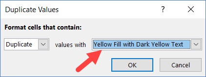
- In the dialog box that has opened, choose the format for highlighting the cells from the drop menu. You can also go for a custom format.
 14")
- When done, click on OK.
 15")
The matching values in both columns will be highlighted in the set format:
 16")
Compare Two Columns & Highlight Mismatching Data
The exact flip on the situation above would be to highlight the values in both columns that do not match. The method is the same as the one we’ve just seen with one small change in the setting.
Using Conditional Formatting, we will highlight unique values in two columns with the steps below:
- Select the values for comparison in both columns.
- Go to the Conditional Formatting menu in the Styles group in the Home Then select Highlight Cell Rules options and Duplicate Values.
- In the drop menu reading Duplicate, select Unique.
- In the second drop menu, choose the format you want the mismatched cells highlighted in.
 18")
- When done, click on the OK
As per the chosen format, the mismatched or unique cells from both columns will be highlighted:
 19")
Compare Two Columns & Pull Matches (Exact Match)
If you were to search for some information from a tiringly long database, you best not opt to do it manually. For example, we have a bunch of event management companies and need to jot down their contact from a vast list of details of event management companies. Let’s see such an example, fairly scaled-down, to give you an idea of how this works.
 20")
In the second table, we have some event management companies and require their contact numbers to be filled. The contact numbers are to be pulled from the first table.
The tool we will use to find the information we require is the VLOOKUP function. The VLOOKUP function looks for a value in a column and returns the value in the same row, from another column. This is the formula we are using for our example:
=VLOOKUP(E3,$B$3:$C$12,2,FALSE)
To begin with, we are searching for the contact for the company mentioned in cell E3. The VLOOKUP function is to locate the company in the first column mentioned in the range B3:C12. It is important to lock the range as absolute references otherwise the reference will keep changing as the formula is copied down.
The «2» in the formula is the number of the column in the mentioned range from which the value is to be pulled. FALSE is used to find an exact match of E3 in column B.
VLOOKUP found an exact match of E3 in row 12 of column B. The corresponding contact was pulled from column C and returned.
 21")
In case the company names mentioned in column E weren’t exact copies of the names mentioned in column B, the formula would return a #N/A error. To make the formula more relenting of small mistakes like an extra space, missing space, a negligible typo, or a forgotten word, change the FALSE in the formula to TRUE. With TRUE in the formula, VLOOKUP will search for an approximate match with the lookup value.
Compare Two Columns & Pull Matches (Partial Match)
If the values you want to look up are vague, TRUE in the VLOOKUP function won’t cover up for it and won’t return the correct information. Don’t worry, you’re still not stuck. There’s a little addition that can save you right. See the formula below for comparing two columns and pulling values using partial matches:
=VLOOKUP("*"&E3&"*",$B$3:$C$12,2,FALSE)
The formula has been copy-pasted from the example earlier with an addition to the lookup value i.e. E3. E3 has been enclosed in & operators and asterisks «*». Let’s say we can’t remember whether the companies have caterers or event management attached to their names. If we can remember at least one word unique to the company name, the asterisk in the formula makes up for the missing characters before and after E3. The & operators add the asterisks to E3.
In the first instance, VLOOKUP is to search for «Appetit» in column B. Cell C4 shows «Bon Appetit Catering». The asterisks have made up for the missing «Bon» from the start of the lookup value and «Catering» from the end of the lookup value.
Having found the partial match of «Appetit» in B4, VLOOKUP pulled the value from column 2 of the range B3:C12 and returned the contact number.
 22")
Compared to all that learning, it’s time for a break. That was all from us on comparing two columns in Excel. Hopefully, with our range of scenarios, you’ll find how to match what and where, or how to not match it, if that’s what you’re aiming for. While you’re finding the right fit for your problem, we’ll be up to all good cracking the Excel enigmas down for you to decipher all its complexities.
Skip to content
На прочтение этой статьи у вас уйдет около 10 минут, а в следующие 5 минут (или даже быстрее) вы легко сравните два столбца Excel на наличие дубликатов и выделите найденные совпадения либо уникальные значения. Ладно, обратный отсчет начался!
Мы все время от времени делаем сравнение данных в Excel. Microsoft Excel предлагает ряд опций для сравнения и сопоставления данных, но большинство из них ориентированы на поиск в одной колонке. Встроенный инструмент удаления дубликатов, доступный в Excel 2019-2010, не может справиться с этой задачей, поскольку он не умеет сравнивать данные между двумя столбиками. Кроме того, он может только удалять дубликаты. Других возможностей — таких как выделение или раскраска, увы, нет :-(.
В этом руководстве мы рассмотрим несколько методов сравнения двух столбцов в Excel и нахождения совпадений и различий между ними.
- Как сравнить 2 столбца построчно?
- Построчное сравнение нескольких столбцов.
- Ищем совпадения и различия в двух столбцах.
- Как извлечь данные для совпадающих значений.
- Выделяем цветом совпадения и различия
- Как выделить цветом уникальные значения и дубликаты в нескольких столбцах сразу?
- Как сопоставить два значения в разных столбцах?
- Быстрый способ сравнить два столбца или списка без формул.
Как сравнить 2 столбца в Excel по строкам.
Когда вы выполняете анализ данных в Excel, одной из наиболее частых задач является сравнение данных нескольких колонок в каждой отдельной их строке. Эту задачу можно выполнить с помощью функции ЕСЛИ , как показано в следующих примерах.
1. Проверяем совпадения или различия в одной строке.
Чтобы выполнить такое построчное сравнение, используйте популярную функцию ЕСЛИ, которая сравнивает первые две ячейки каждого из них. Введите её в какой-либо другой столбик той же строки, а затем скопируйте ее вниз, перетащив маркер заполнения (маленький квадрат в правом нижнем углу). При этом курсор изменится на знак плюса:

Чтобы найти в соответствующей строке позиции с одинаковым содержимым, A2 и B2 в этом примере, запишите:
=ЕСЛИ(A2=B2; «Совпадает»; «»)
Чтобы найти позиции в одной строке с разным содержимым, просто замените «=» знаком неравенства:
=ЕСЛИ(A2<>B2; «НЕ совпадает»;””)
И, конечно же, ничто не мешает найти совпадения и различия с помощью одной формулы:
=ЕСЛИ(A2=B2; «Совпадает»; «НЕ совпадает»)
Результат может выглядеть примерно так:

Как видите, одинаково хорошо обрабатываются числа, даты, время и текст.
2. Сравниваем построчно с учетом регистра.
Как вы, наверное, заметили, формулы из предыдущего примера игнорируют регистр при сравнении текстовых значений, как в строке 10 на скриншоте выше. Если вы хотите найти совпадения с учетом регистра, используйте функцию СОВПАД (EXACT в английской версии):
=ЕСЛИ(СОВПАД(A2; B2); «Одинаковый»; «»)

Чтобы найти различия с учетом регистра в одной строке, введите соответствующий текст («Уникальный» например) в третий аргумент функции ЕСЛИ:
=ЕСЛИ(СОВПАД(A2; B2); «Одинаковый»; «Уникальный»)
Сравните несколько столбцов построчно
Мы можем ставить перед собой следующие цели:
- Найти строки с одинаковыми значениями во всех из них.
- Найти строки с одинаковыми значениями в любых двух.
Пример 1. Найдите полное совпадение по одной строке.
Если в вашей таблице три или более колонки, и вы хотите найти строки с одинаковыми записями во всех из них, функция ЕСЛИ с оператором И подойдет для вас:
=ЕСЛИ(И(A2=B2; A2=C2); «Полное совпадение»; «»)

Если в вашей таблице очень много колонок, более элегантным решением будет использование функции СЧЁТЕСЛИ :
=ЕСЛИ(СЧЁТЕСЛИ($A2:$C2; $A2)=3; «Полное совпадение»; «»)
где 3 — количество сравниваемых колонок.
Или можно использовать —
=ЕСЛИ(СЧЁТЕСЛИ($A2:$C2; $A2)=СЧЁТЗ(A2:C2); «Полное совпадение»; «»)
Пример 2. Найдите хотя бы 2 совпадения в данных.
Если вы ищете способ сравнить данные на предмет наличия любых двух или более ячеек с одинаковыми значениями в одной строке, используйте функцию ЕСЛИ с оператором ИЛИ:
=ЕСЛИ(ИЛИ(A2=B2; B2=C2; A2=C2); «Найдены одинаковые»; «»)

Если есть много данных для сравнения, ваша конструкция с оператором ИЛИ может стать слишком громоздкой. В этом случае лучшим решением было бы добавить несколько функций СЧЁТЕСЛИ. Первый СЧЁТЕСЛИ подсчитывает, сколько раз текущее значение из первой колонки встречается во всех данных, находящихся правее него, второй СЧЁТЕСЛИ определяет то же самое для значения из второй колонки, и так далее. Если счетчик равен 0, возвращается надпись «Все уникальные», в противном случае — «Найдены одинаковые». Например:
=ЕСЛИ(СЧЁТЕСЛИ(B2:D2;A2)+СЧЁТЕСЛИ(C2:D2;B2)+(C2=D2)=0;»Все уникальные»;»Найдены одинаковые»)

Могу предложить также более компактный вариант выявления совпадений — формула массива:
{=ЕСЛИ(СУММ(СЧЁТЕСЛИ(A2:D2;A2:D2))>4;»Совпадения»;»»)}
или
{=ЕСЛИ(СУММ(СЧЁТЕСЛИ(A2:D2;A2:D2))>СЧЁТЗ(A2:D2);»Совпадения»;»»)}
Попробуйте — получите тот же результат. Также не забудьте нажать Ctrl + Shift + Enter, чтобы ввести всё правильно.
Как сравнить два столбца в Excel на совпадения и различия?
Предположим, у вас есть 2 списка данных в Excel, и вы хотите найти все значения (числа, даты или текстовые записи), которые находятся в колонке A, но их нет в B. То есть, исходные данные из А мы сравниваем с В.
Для этого вы можете встроить функцию СЧЁТЕСЛИ($B:$B;$A2)=0 в логический тест ЕСЛИ и проверить, возвращает ли она ноль (совпадение не найдено) или любое другое число (найдено хотя бы 1 совпадение).
Например, следующая формула ЕСЛИ/СЧЁТЕСЛИ выполняет поиск значения из A2 по всему столбцу B. Если совпадений не найдено, возвращается «Нет совпадений в B», в противном случае — пустую строку:
=ЕСЛИ(СЧЁТЕСЛИ($B:$B; $A2)=0; «Нет совпадений в В»; «»)

Тот же результат может быть достигнут при использовании функции ЕСЛИ всесте с ЕОШИБКА и ПОИСКПОЗ:
=ЕСЛИ(ЕОШИБКА(ПОИСКПОЗ($A2;$B$2:$B$10;0));»Уникальное»; » Найдено в B»)
Или, используя следующую формулу массива (не забудьте нажать Ctrl + Shift + Enter, чтобы ввести ее правильно):
=ЕСЛИ(СУММ(—($B$2:$B$10=$A2))=0; «»;» Найдено в B»)
Если вы хотите, чтобы одно выражение определяло как дубликаты, так и уникальные значения, поместите текст совпадений в пустые двойные кавычки («») в любой из приведенных выше формул. Например:
=ЕСЛИ(СЧЁТЕСЛИ($B:$B; $A2)=0; «Уникальное»; «Дубликат»)
Думаю, вы понимаете, что точно таким же образом можно наоборот сравнивать В с А.
Как сравнить два списка в Excel и извлечь совпадающие данные?
Иногда вам может потребоваться не только сопоставить две колонки в двух разных таблицах, но и извлечь соответствующие записи из второй таблицы. В Microsoft Excel предусмотрена специальная функция для этих целей — функция ВПР.
Кроме того, в отдельной статье мы подробно рассмотрели 4 способа, как сравнить таблицы при помощи формулы ВПР.
В качестве альтернативы вы можете использовать более мощную и универсальную комбинацию ИНДЕКС и ПОИСКПОЗ.
Например, следующее выражение сравнивает названия продуктов в колонках D и A, и если совпадение найдено, соответствующая цифра продаж извлекается из B. Если совпадения не найдено, возвращается ошибка #Н/Д.
=ИНДЕКС($B$2:$B$6;ПОИСКПОЗ($D2;$A$2:$A$6;0))
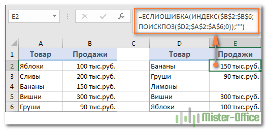
Сообщение об ошибке в таблице выглядит не слишком красиво. Поэтому обработаем это выражение при помощи ЕОШИБКА:
=ЕСЛИОШИБКА(ИНДЕКС($B$2:$B$6;ПОИСКПОЗ($D2;$A$2:$A$6;0));»»)
Теперь мы видим либо число, либо пустое значение. Никаких ошибок.
Как выделить совпадения и различия в 2 столбцах.
Когда вы сравниваете наборы данных в Excel, вы можете захотеть «визуализировать» элементы, которые присутствуют в одном, но отсутствуют в другом. Вы можете закрасить такие позиции любым цветом по вашему выбору с помощью формул. И вот несколько примеров с подробными инструкциями.
1. Выделите совпадения и различия построчно.
Чтобы сравнить два столбца в Excel и выделить те позиции в первом, которые имеют идентичные записи во втором по той же строке, выполните следующие действия:
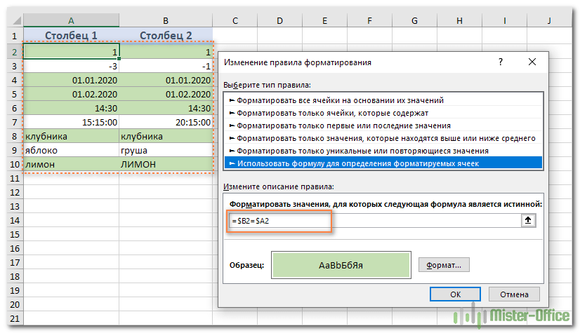
- Выберите область, в которой вы хотите выделить.
- Щелкните Условное форматирование> Новое правило…> Используйте формулу.
- Создайте правило с простой формулой, например =$B2=$A2 (при условии, что строка 2 является первой строкой с данными, не включая заголовок таблицы). Пожалуйста, дважды проверьте, что вы используете относительную ссылку на строку (без знака $), как записано выше.
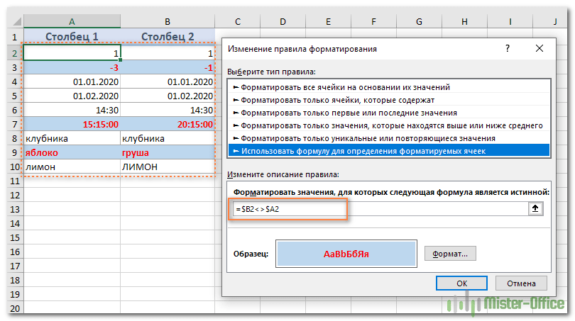
Чтобы выделить различия между колонками A и B, создайте правило с формулой =$B2<>$A2
Если вы новичок в условном форматировании Excel, смотрите пошаговые инструкции в статье Как закрасить строку или столбец по условию.
2. Выделите уникальные записи в каждом столбце.
Когда вы сравниваете два списка в Excel, вы можете выделить 3 типа элементов:
- Предметы только в первом списке (уникальные)
- Предметы только во втором списке (уникальные)
- Элементы, которые есть в обоих списках (дубликаты).
О выделении дубликатов — смотрите пример выше. А сейчас рассмотрим, как выделить неповторяющиеся элементы в каждом из списков.
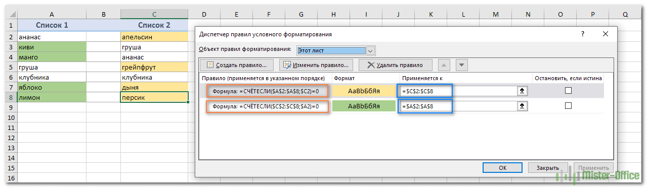
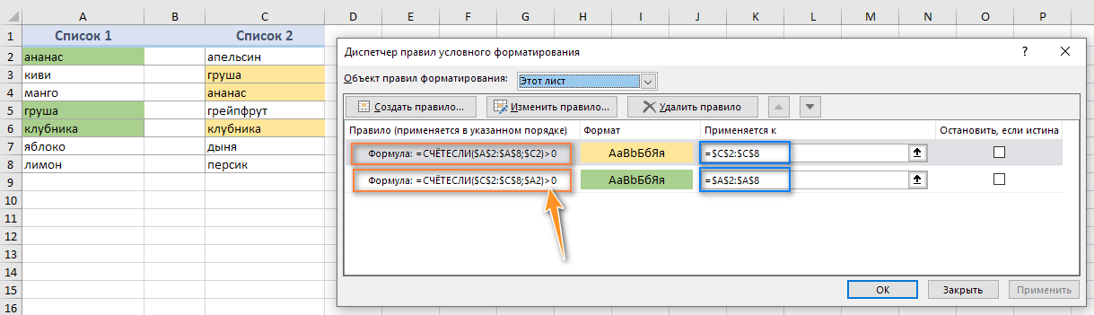
Предположим, что ваш список 1 находится в колонке A (A2:A8), а список 2 — в колонке C (C2:C8). Вы создаете правила условного форматирования с помощью следующих формул:
Выделите уникальные значения в списке 1 (столбик A): =СЧЁТЕСЛИ($A$2:$A$8;C$2)=0
Выделите уникальные значения в списке 2 (столбик C): =СЧЁТЕСЛИ($C$2:$C$8;$A2)=0
И получите следующий результат:
3. Выделите дубликаты в 2 столбцах.
Если вы внимательно следовали предыдущему примеру, у вас не возникнет трудностей с настройкой СЧЁТЕСЛИ, чтобы она находила совпадения, а не различия. Все, что вам нужно сделать, это установить счетчик больше нуля:
Вновь используем условное форматирование при помощи формулы.
Выделите совпадения в списке 1 (столбик A): =СЧЁТЕСЛИ($A$2:$A$8;C$2)>0
Выделите совпадения в списке 2 (столбик C): =СЧЁТЕСЛИ($C$2:$C$8;$A2)>0
Выделите цветом различия и совпадения в нескольких столбцах
При сравнении значений в нескольких наборах данных построчно, самый быстрый способ выделить одинаковые — создать правило условного форматирования. А самый быстрый способ скрыть различия — воспользоваться инструментом «Выделить группу ячеек», как показано в следующих примерах.
1. Как выделить совпадения.
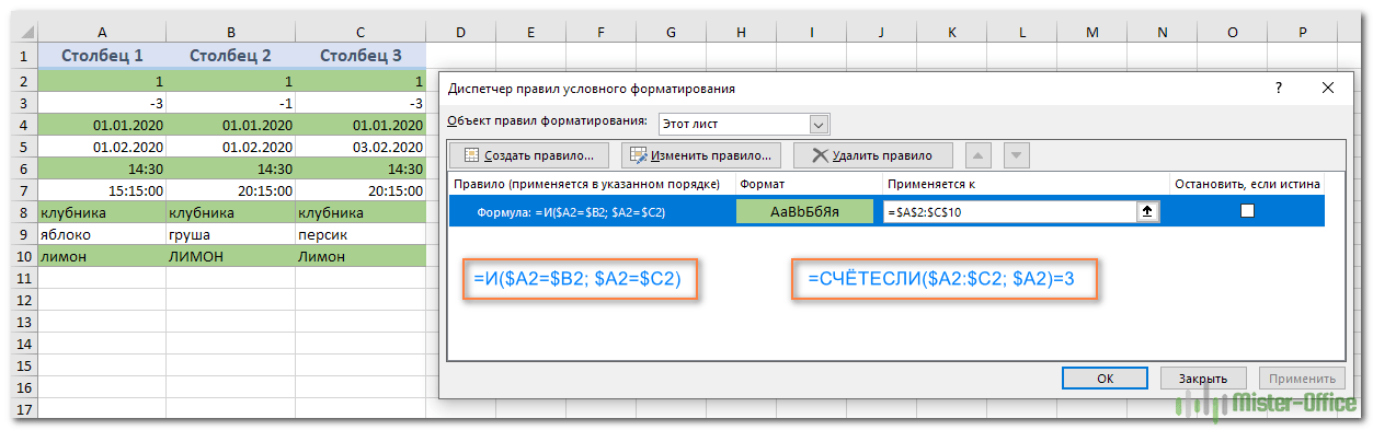
Чтобы выделить строки, которые имеют одинаковые значения по всей длине, создайте правило условного форматирования на основе одного из следующих выражений:
=И($A2=$B2; $A2=$C2)
или
=СЧЁТЕСЛИ($A2:$C2; $A2)=3
Где A2, B2 и C2 — самые верхние в вашем диапазоне, а 3 — количество колонок для сравнения.
Конечно, можно не ограничиваться сравнением только 3 колонок. Вы можете использовать аналогичные формулы для выделения строк с одинаковыми значениями в 4, 5, 6 или более столбиках.
И еще один способ выделения цветом повторяющихся значений в нескольких столбцах. Снова используем условное форматирование. Выделяем нужную область, затем на ленте в меню условного форматирования выбираем Правила выделения ячеек — Повторяющиеся значения. Определяем желаемое оформление, получаем картину подобную той, что вы видите ниже.
Кстати, на последнем этапе вы можете выбрать не повторяющиеся, а уникальные значения. Способ, конечно, незамысловатый, но, возможно, он вам будет полезен.
2. Как выделить различия.
Чтобы быстро выделить позиции с разными значениями в каждой отдельной строке, вы можете использовать функцию Excel «Выделить группу ячеек».
- Выберите диапазон ячеек, который вы хотите сравнить. В этом примере я выбрал диапазон от A2 до C10.
По умолчанию самая верхняя координата выбранного диапазона является активной ячейкой, и все значения в той же строке будут сравниваться с нею. Она при выделении области имеет белый цвет, а все остальные ячейки выбранного диапазона выделены серым. В этом примере активной является A2, поэтому столбец сравнения — A.
Чтобы изменить столбец сравнения, используйте клавишу TAB для перемещения по диапазону слева направо или клавишу Enter для перемещения сверху вниз. Если нужно перемещаться снизу вверх, то нажмите и удерживайте SHIFT, и вновь используйте ТАВ — будете двигаться не вниз, а вверх. Вы увидите, как ваше белое пятно перемещается, и соответственно изменяется активный столбец.
- На вкладке «Главная» нажмите «Найти и выделить» > « Выделить группу ячеек». Затем выберите «Отличия по строкам» и нажмите «ОК» .
- Позиции, значения которых отличаются от ячеек сравнения в каждой строке, выделяются. Если вы хотите закрасить выделенные ячейки каким-либо цветом, просто щелкните значок «Цвет заливки» на ленте и выберите нужный цвет.
Как сравнить два значения в отдельных столбцах.
Фактически, сравнение двух ячеек — частный случай сравнения двух колонок в Excel построчно, за исключением того, что вам не нужно копировать формулы.
Например, для сравнения ячеек A1 и C1 можно использовать:
Для совпадений: =ЕСЛИ(A1=C1; «Совпадает»; «»)
Для различий: =ЕСЛИ(A1<>C1; «Уникальные»; «»)
Чтобы узнать о некоторых других способах сравнения ячеек в Excel, см. Как сравнивать значения в ячейках Excel .
Для более эффективного анализа данных вам могут потребоваться более сложные формулы, и вы можете найти несколько хороших идей в следующих руководствах:
- Использование функции ЕСЛИ в Excel
- Функция ЕСЛИ: проверяем условия с текстом
Быстрый способ сравнения двух столбцов или списков без формул.
Теперь, когда вы знаете, что предлагает Excel для сравнения и сопоставления столбцов, позвольте мне продемонстрировать вам альтернативное решение, которое может сравнить 2 списка с разным количеством столбцов на предмет дубликатов (совпадений) и уникальных значений (различий).
Надстройка Ultimate Suite умеет искать идентичные и уникальные записи в одной таблице, а также сравнивать две таблицы, находящиеся на одном листе или в двух разных листах или даже в разных книгах.
В рамках этой статьи мы сосредоточимся на функции под названием «Сравнить таблицы (Compare Tables)» , которая специально разработана для сравнения двух списков по любым указанным вами столбцам. Сравнение двух наборов данных по нескольким столбцам является реальной проблемой как для формул Excel, так и для условного форматирования, но этот инструмент легко справляется с этим.
Для начала рассмотрим самый простой случай – сравним два столбца на совпадения и различия.
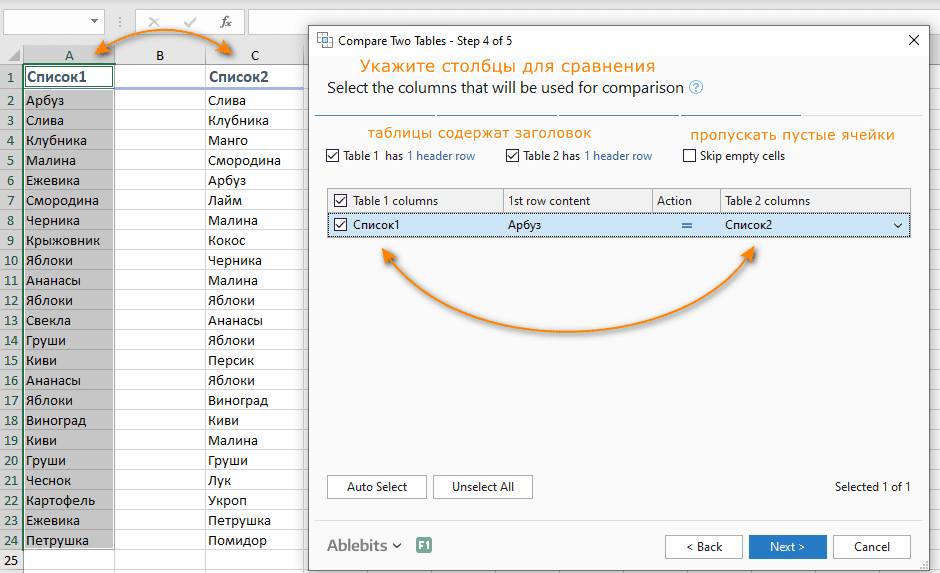
Предположим, у нас имеется два списка товаров. Нужно сравнить их между собой, как ранее мы делали при помощи формул.

Запускаем инструмент сравнения таблиц и выбираем первый столбец. При необходимости активируем создание резервной копии листа.

На втором шаге выбираем второй столбец для сравнения.

На третьем шаге нужно указать, что именно мы ищем – дубликаты либо уникальные значения.

Далее указываем столбцы для сравнения. Поскольку столбцов всего два, то здесь все достаточно просто:
На пятом шаге выберите, что нужно сделать с найденными значениями – удалить, выбрать, закрасить цветом, скопировать либо переместить. Можно добавить столбец статуса подобно тому, как мы это делали ранее при помощи функции ЕСЛИ. С использованием формул вы кроме того сможете разве что закрасить ячейки. Здесь же диапазон возможностей гораздо шире. Но мы выберем простой и наглядный вариант – заливку ячеек цветом.

Ячейки списка 1, дубликаты которых имеются в списке 2, будут закрашены цветом.
А теперь повторим все описанные выше шаги, только будем сравнивать список 2 с первым. И вот что мы в итоге получим:

Не закрашенные цветом ячейки содержат уникальные значения. Красиво и наглядно.
А теперь давайте попробуем сравнить сразу несколько столбцов. Допустим, у нас есть два экземпляра отчёта о продажах. Они расположены на разных листах нашей книги Excel. Список товаров совершенно одинаков, а вот сами цифры продаж отличаются кое-где.

Действуя совершенно аналогичным образом, как это было описано выше, выбираем эти две таблицы для сравнения. На третьем шаге выбираем поиск уникальных значений, чтобы можно было выбрать и выделить именно несовпадения в данных.
Устанавливаем соответствие столбцов, как это показано на рисунке ниже.

Для наглядности вновь выбираем заливку цветом для несовпадающих значений.
И вот результат. Несовпадающие строки закрашены цветом.

Если вы хотите попробовать этот инструмент, вы можете загрузить его как часть надстройки Ultimate Suite for Excel.
Вот какими способами вы можете сравнить столбцы в Excel на наличие дубликатов и уникальных значений.
Если у вас есть вопросы или что-то осталось неясным, напишите мне комментарий, и я с радостью уточню это подробнее. Спасибо за чтение!
 Функция ЕСЛИОШИБКА – примеры формул — В статье описано, как использовать функцию ЕСЛИОШИБКА в Excel для обнаружения ошибок и замены их пустой ячейкой, другим значением или определённым сообщением. Покажем примеры, как использовать функцию ЕСЛИОШИБКА с функциями визуального…
  9 способов сравнить две таблицы в Excel и найти разницу — В этом руководстве вы познакомитесь с различными методами сравнения таблиц Excel и определения различий между ними. Узнайте, как просматривать две таблицы рядом, как использовать формулы для создания отчета о различиях, выделить…
  Сравнение ячеек в Excel — Вы узнаете, как сравнивать значения в ячейках Excel на предмет точного совпадения или без учета регистра. Мы предложим вам несколько формул для сопоставления двух ячеек по их значениям, длине или количеству…
  Вычисление номера столбца для извлечения данных в ВПР — Задача: Наиболее простым способом научиться указывать тот столбец, из которого функция ВПР будет извлекать данные. При этом мы не будем изменять саму формулу, поскольку это может привести в случайным ошибкам.…
  Как проверить правильность ввода данных в Excel? — Подтверждаем правильность ввода галочкой. Задача: При ручном вводе данных в ячейки таблицы проверять правильность ввода в соответствии с имеющимся списком допустимых значений. В случае правильного ввода в отдельном столбце ставить…
  Функция ЕСЛИ: проверяем условия с текстом — Рассмотрим использование функции ЕСЛИ в Excel в том случае, если в ячейке находится текст. СодержаниеПроверяем условие для полного совпадения текста.ЕСЛИ + СОВПАДИспользование функции ЕСЛИ с частичным совпадением текста.ЕСЛИ + ПОИСКЕСЛИ…
  Визуализация данных при помощи функции ЕСЛИ — Функцию ЕСЛИ можно использовать для вставки в таблицу символов, которые наглядно показывают происходящие с данными изменения. К примеру, мы хотим показать в отдельной колонке таблицы, происходит рост или снижение продаж.…
 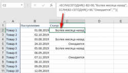 3 примера, как функция ЕСЛИ работает с датами. — На первый взгляд может показаться, что функцию ЕСЛИ для работы с датами можно применять так же, как для числовых и текстовых значений, которые мы только что обсудили. К сожалению, это…
When dealing with Data analytics, comparing data populated in two or more columns is common practice.
Manually comparing data could take hours or even days, depending on the amount of the data in question.
But when it comes to using Excel, you can expect data work to be done in a matter of minutes
The same is true for comparing two columns in Excel.
Let’s see the versatility of Excel’s features for comparing two columns through the article below.
You may want to Compare Columns in Excel to find matching, or non matching data, or simply to pull out specific information.
The first step to compare columns typically involves comparing data by sorting it into two or more adjacent columns.
This is one of the quickest techniques in Excel and can compare any amount of data in less than a second.
Use Cases of Comparing Columns
Comparing two data columns having 5 or 10 entries is a piece of cake, but what if you have thousands of data entries in both columns?
In case you are a beginner, let’s first familiarize ourselves with what the comparison of two columns in Excel is used for.
We have listed some use cases below:
- Maybe you want to find the top-selling mobile phones at your store – you can compare the sales of mobile phone data to find the top selling phone.
- Perhaps you want to find out which of your favorite football players qualified for a tournament – here you can compare your favorite players with qualified players and find out.
- If you want to know the availability of certain gadgets from a huge list of items at your store – you can fetch the data by comparing your required items with the store inventory.
- Similarly, you can find out the share price of your stock by comparing it with the stock data in a few clicks!
There are hundreds of other cases which involve comparing columns. It is fairly simple to use, and we have demonstrated the major ways to compare data for decision making as follows:
Compare Two Columns – Exact Row Match
When comparing two cells, Excel matches each row of the first column against the second column to find the similarities or differences.
The top four methods for comparing two columns are listed below:
- Method # 1: Compare two columns using a Simple Formula
- Method # 2: Compare two columns using IF Function
- Method # 3: Compare two columns using EXACT Function
- Method # 4: Compare two columns using conditional formatting
Let’s explore these methods and related examples below:
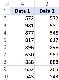
Compare Two Columns Using a Simple Formula
Look at the following datasheet. It reflects the record of 10 employees in an organization displaying their log-in and log-out time. Column A represents the names of the employees, whereas Column B and Column C display their log-in and log-out times, respectively.
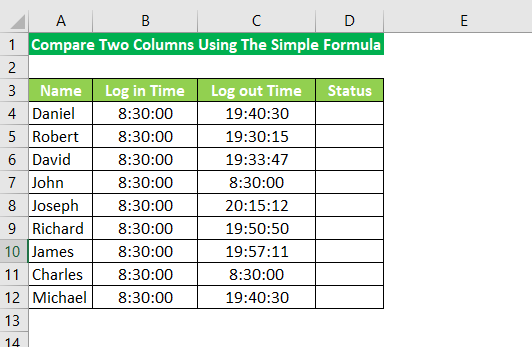
In this example, our objective will be to highlight the employees who forgot to log out using a simple Excel technique. Since the office timings begin from 8:30, so the employees who didn’t log out will have the same log-in and log-out time. Let’s now compare the columns and see the results.
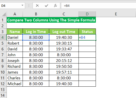
We use the comparison operator “=” (equal to) to find the exact match in two columns. It is used as follows:
Step 1
In cell D4, enter the operator “=” in the formula bar and select cell B4.
Step 2
Enter the “=” operator again, followed by selecting cell C4.
Step 3
Now press the “Enter” key. You get a “false” value in return; this implies that the value in cell B4 is not equal to that of cell C4.
Step 4
Now drag the cell handle or copy-paste the formula to the remaining cells. The output will be either “True” or “False,” as shown in the figure above.
Assuming that the value in column B is equal to the value in column C, you obtain “True” in the result and vice versa.
Here, ‘True’ means that the log-in and log-out time match, which in turn suggests that the employee forgot to log out. In contrast, False means that the log-in and log-out entries do not match each other.
Hence, as evident from the gif, two employees, John and Charles, did not log out properly.
Note: You may employ the filter function to immediately sort out the rows with the corresponding value ‘True’ in column D. This will help you filter out the employees who forgot to log out.
Compare Two Columns Using the IF Function
Considering the above example again, let’s now compare the two columns, B and C, using the IF Function. The result of the comparison must be something like this:
-
- “Forgot log out” if the employee forgot to log out
- “OK,” if the employee logs out properly
The syntax of the IF function for this comparison is as follows:
=IF (B4=C4,“Forgot log out”,“Ok”)
Since the IF function makes a logical comparison between two values, let’s see how the formula works before getting into its example.
The IF Function compares two columns, and if the values match, the Function returns “True”; otherwise, it returns “False.” Now for every “True” value, it displays a specific text.
In this case, Excel displays the message, “Forgot log out,” for every true argument. Similarly, the formula is set to return the message “Ok” for every “False” value.
Let’s apply it to our data as follows:
Step 1
Put the above IF Function in cell E4 and press Enter to get the output.
Step 2
Drag the cell handle or copy-paste the cell formula into the remaining cells to obtain the output.
The Function displays Forgot log-out message where both the values in the cells match and displays OK, where the values are different.
This Function can be pretty helpful when dealing with a large list of items and matching their properties.
Compare Two Columns Using the EXACT Function
Considering the data in the above example again, let’s use the EXACT Function to compare two columns.
The syntax of the EXACT Function is as follows:
=EXACT (B4, C4)
Step 1
Put the above Exact formula in the output cell F4.
Step 2
Press the Enter key to get the following result.
Step 3
Drag the cell handle to copy the formula in the remaining cells.
Comparing both columns with the EXACT Function shows two true cases where John and Charles forgot to log out properly.
Tip: Note that the Exact Function is case sensitive, i.e., treats uppercase and lowercase characters differently.
Comparing Two Columns Under Effect of EXACT Function’s Case Sensitivity
To see how the EXACT Function works with case sensitive data, let’s see the example below:
Using the same data as in the above examples, we changed the letter case of the names. Let’s now compare both the columns using the EXACT Function. The syntax of the EXACT Function looks something like this:
=EXACT (A4, B4)
Step 1
Insert the syntax in the formula bar by selecting cell E4 and pressing Enter. The result will be displayed in the cell as:
Step 2
Drag the cell handle to copy the EXACT formula in the remaining cells.
As evident from the image above, the EXACT Function returns “False” when the casing of Cell A is different from Cell B and vice versa.
Compare Two Columns Using Conditional Formatting
Another feasible method is using conditional formatting. It comes in handy when you want to compare data in two columns and do not want the result to be displayed in the third column. You can find the matching entries within the two columns using conditional formatting.
Consider the following example:
To highlight the matching columns in the above image, follow the steps given below:
Step 1
CTRL+A to select the entire data. In the “Home” tab, select “Conditional formatting.” From the drop-down list, select “New Rule,” and the “New Formatting Rule” window appears.
Step 2
From the new formatting rule dialog box, select “Use a formula to determine which cells to format.” The drop-down list will expand to get the formula for the cell formatting.
Step 3
Now enter the formula “=$B4=$C4” under the “edit the rule description.”
Step 4
Once done, click the “format” button, and a Format Cell window will appear. From the format Cell window, select the “Fill” option from the top menu and select the color that you want to fill in the identical columns. Click the “Ok” button twice, and you’re done.
The matching entries of columns B and C are highlighted as shown in the figure below:
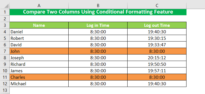
It is clear from the results that the log-in and log-out columns of John and Charles are identical, indicating that their log-out time was different than others. This is how you can use the conditional formatting feature to compare data using your customized formulas to get the desired results.
Compare Two Columns – Highlight Matching Data
Like the method above, you can use conditional formatting to compare two columns by comparing each cell of both columns and not involving a row-by-row comparison.
Consider the following example:
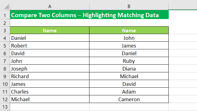
To highlight the matching data in two columns, follow these steps:
Step 1
Select the entire data set and from the “Home” tab, select “Conditional formatting.” In the drop-down list, hover the cursor over the “Highlight Cell Rules” and select “Duplicate Values” from the list. From the Duplicate Value pop-up window, select the color scheme that fills the cell matching in both columns. Once done, press OK.
The result will be something like in the image below:
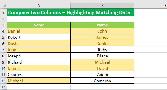
The conditional formatting function highlights the matching entries in both columns.
Tip: Must note how the Conditional Formatting duplicate rule is not case sensitive. Therefore, conditional formatting can be used to compare two columns if case sensitivity is not your concern.
Compare Two Columns – Find Missing Data
You can use any of the two methods below to find any mismatched data in your column set. These involve Excel formulas and formatting features making the process quick and fun.
1 – Finding Mismatched Data Using Formula
The first method is based on the use of a formula to find mismatched values. For that, let’s see the example below.
Step 1
Select the entire data set. Go to the “Home” tab and click the “Conditional formatting” tab. From the drop-down list, select the “New Rule” option and from the “New Formatting Rule” window, select “use a formula to determine which cells to format.”
Step 2
To highlight the mismatched values, enter the following formula in the Edit formatting rule dialogue box under the box that reads “Format values where this formula is true”.
=$A4<>$B4
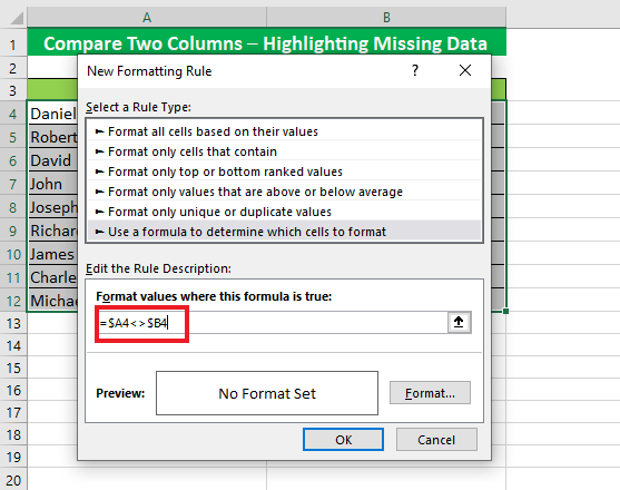
Step 3
Click the “Format” button to select your desired color for mismatched data, and choose the color from the “Format Cell” window. Press the “Ok” button twice, and tada! You’re done.
The highlighted cells are visible in the image below:
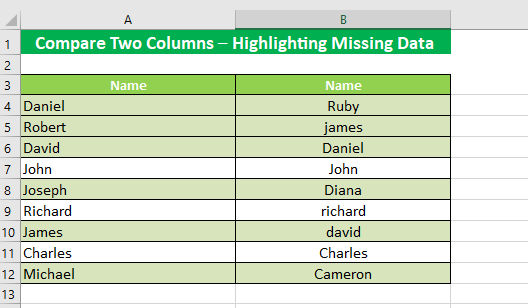
In the above image, all the mismatching rows in both columns have been highlighted using Conditional Formatting, whereas the matching data remains unchanged.
2 – Finding Mismatched Data Using Conditional Formatting
Excel also offers features that help you find data in a single column. We use conditional formatting for this method as well.
Consider the following example:

Step 1
Select the entire data. Go to the “Home” tab and then select the “Conditional Formatting” tab. Move the cursor on the “Highlight Cell Rules” and select the “Duplicate Values” option from the drop-down list. You get the “Duplicate Values” window on your screen as follows:
Step 2
Select the option “Unique” and specify the formatting for those unique data.
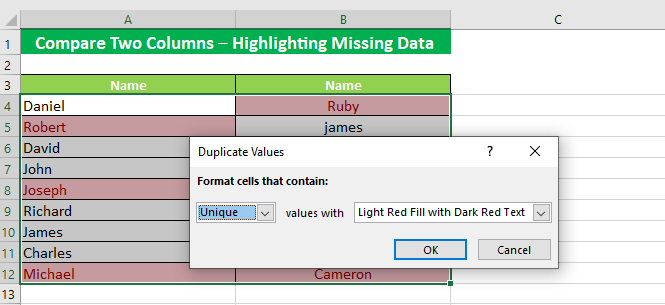
Step 3
Press “Ok” to get the results.
The image displays unique data highlighted in both columns as below:
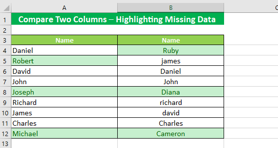
Since the Conditional Formatting feature is not case sensitive, it considers “David” and “david” the same entries. However, if your work calls for dealing with case-sensitive data, you can go for the other diverse options mentioned in this article.
Compare Two Columns – VLOOKUP
When you want to compare two columns in Excel, the VLOOKUP function is the king. It offers multiple options to compare data. Let us see how to use the VLOOKUP function to its full potential while comparing two columns.
Consider the following example:
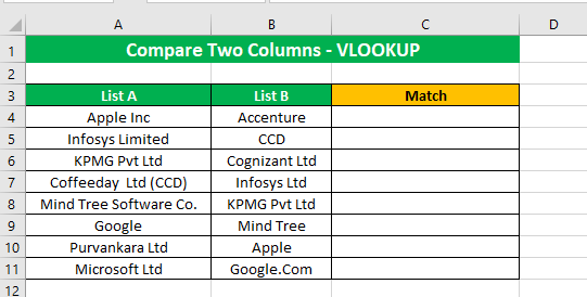
The above image displays two lists of various companies’ names. We will use the VLOOKUP Function to compare the columns and find the matching entries.
Step 1
Let us suppose we want to compare List A to List B to find the common names in both columns. Here is how we can use the VLOOKUP function for the said purpose.
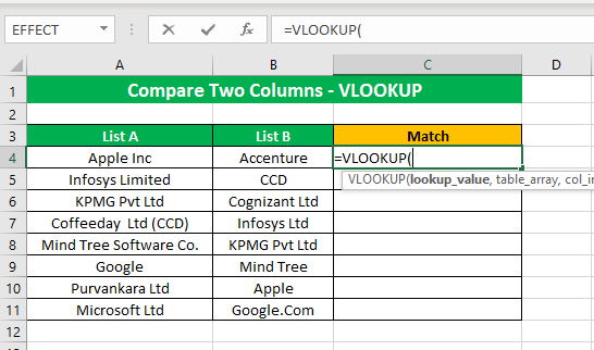
Step 2
Insert cell B4 in the VLOOKUP formula as we want the values in List B to be looked up.
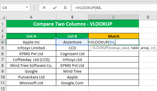
Step 3
In the next argument, the Table array (where the values are to be looked up for) is set to List A. Select the range of cells from A4 to A11 and make it an absolute cell reference by pressing F4.
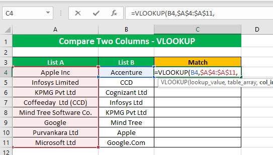
Step 4
The next argument is the “Col Index Num,” number of the column from left to right from which the result is to be obtained. Since List A consists of only one column, so the “Col Index Num” will be 1. Insert this value in the Function.
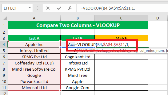
Step 5
The fourth and last argument to the VLOOKUP function is an optional one. You may set it to FALSE or leave it omitted to Excel to set it to FALSE by default.
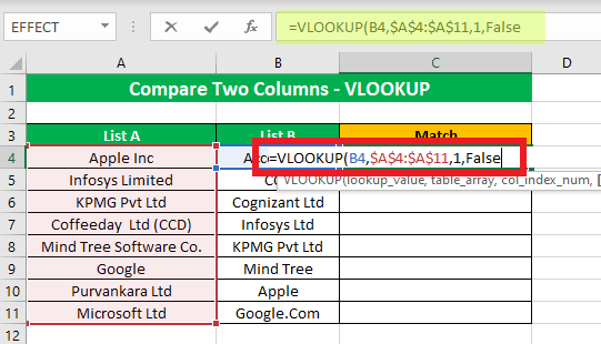
Step 6
Once you’re done with the Function, close the bracket and press “Enter” to get the results.
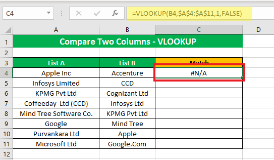
It is clear from the result that the cell value Accenture is not available in List A. #N/A equates to the fact that the values do not match.
Step 7
Drag the cell handle and copy the VLOOKUP function in the remaining cells.

VLOOKUP facilitates a quick comparison of data populated within both columns.
However, in the case of ‘no match, it returns the error “#N/A”. This may confuse inexperienced users, making them think that something is wrong with the formula.
To remove this Error message, replace it with a blank by using the IFNA function. The syntax of the IFNA function for this comparison will be something like this:
=IFNA(=VLOOKUP(B4,$A$4:$A$11,1,FALSE),””)
Step 8
Insert the IFNA function in the above example and press “Enter.”
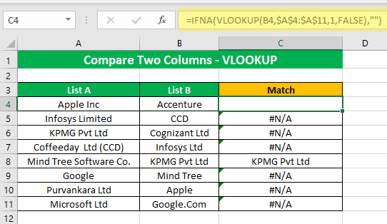
Step 9
Drag the cell handle to copy-paste the IFNA function in the remaining cells. The result should look something like this:
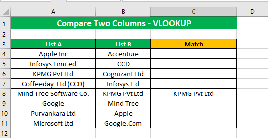
It is evident from the image above that “KPMG Pvt Ltd” is the only company name that exactly matches both columns.
Using VLOOKUP For Partially Comparing Two Columns
In the above example, a few names exist in both the columns but are followed by suffixes or prefixes.
Until the values are in absolute conformity (letting aside the letter case), Excel matching or comparing functions would fail to fetch the desired results.
However, the VLOOKUP function has the capability of handling such situations using the “Wildcard Characters.”
You can use the wildcard character (*) that enables the VLOOKUP Function to look up values before and after the selected data. Let us see the use of (*) to get the desired match.
Step 1
Modify the above formula and add (*) as given below:
=IFNA(VLOOKUP(“*”&B4&”*”,$A$4:$A$11,1,FALSE),””)
Step 2
Drag the cell handle to copy-paste the formula into the remaining cells. The result will look something like this:
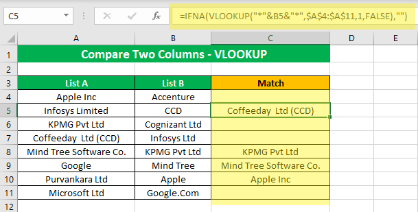
Before using the wildcard character ‘asterisk,’ Excel returned only one match, but upon using the wildcard character, the formula returned three more matches. Weird, no?
Let’s see the science behind this change.
The wildcard character asterisk matches any number of characters. As we applied the asterisk before and after the data value of each cell of list B, it returned every entry from List A that had the text string from List B.
For example, cell B5 contains CCD, whereas A7 contains “Coffeeday Ltd (CCD)”. Using the wildcard character ‘asterisk’ matches and gives back all results from Column A that have the text string CCD.
The same is true for “Mind Tree” and “Apple” present in B9 and B10.
Here’s how seamless the process is.
Compare Two Columns – Pull Matching Data
Comparing two columns in Excel is a normal practice and is usually utilized in making administrative decisions. By comparing the data columns, you can pull out information to analyze the data, and the VLOOKUP function is extremely helpful when it comes to matching data. Let us now see how you can use VLOOKUP to draw the matching data in another column.
Consider the following example:
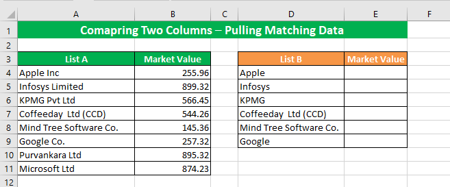
List A consists of companies’ names, whereas the Market Value column contains their market price, respectively. Suppose we want to fetch the market value for List B. To do that, we will use the VLOOKUP Function to find values in List A and then fetch the corresponding market value from List B.
Step 1
Insert the VLOOKUP formula in cell E4.
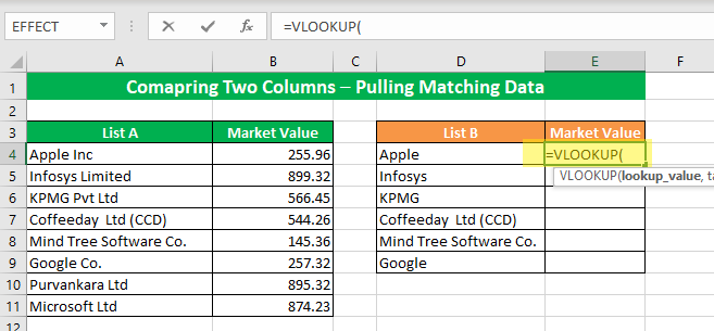
Step 2
We want to look up the market value of the companies from List B, so we select cell D4 as the lookup value.
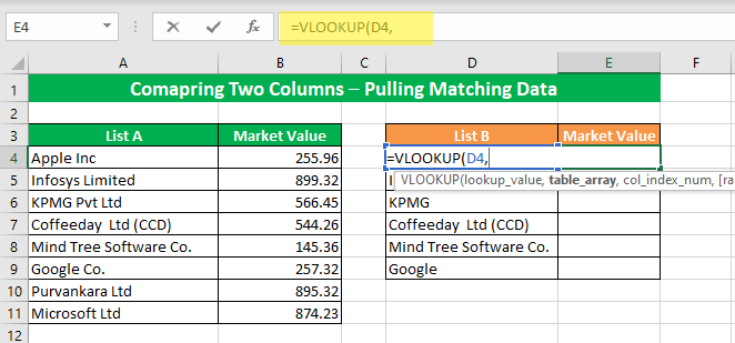
Step 3
Since we want to find the market values of the selective companies from List A, we select the “Table array” range from A4 to B11 and make the cell reference absolute by pressing F4.
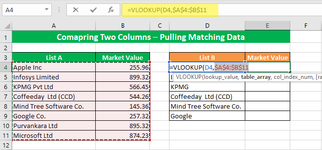
Step 4
To fetch the market price of the selective companies, we insert the column index of the market value data column, which is 2.
Notably, the Column Index is counted from left to right in the selected table array.

Step 5
We enter False or 0 as the last argument in the VLOOKUP Function for an exact match to obtain the results.
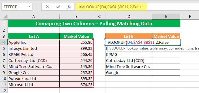
Step 6
Once done with the VLOOKUP formula, close the bracket. Since we have learned in the previous example that the VLOOKUP function returns a #Num error for a mismatch, you may want to nest the above Function into the IFNA function for better results.
The formula will look something like this:
=IFNA(VLOOKUP(D4,$A$4:$B$11,2,False),””)
Now put this formula in cell E4 and press “Enter” to get the results.
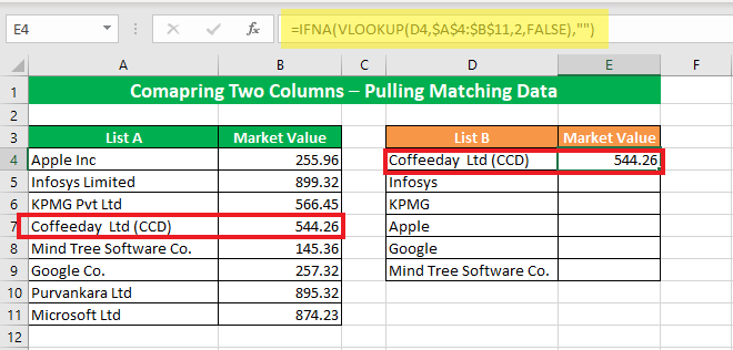
Step 7
Drag the cell handle to copy-paste the VLOOKUP formula into the remaining cells.
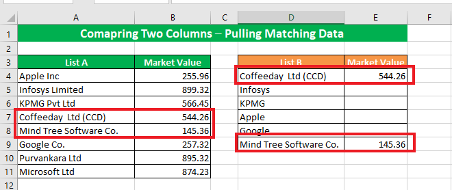
Pulling Matching Data with Partial Match Using VLOOKUP Function
The above example represents the instance where the VLOOKUP function matched and returned the values that were an absolute match.
However, it did not work the same for “Apple” and “Apple Inc.” Here’s what you can do to look up values having prefixes or suffixes.
In the previous example, we learned how to use the wildcard characters to fetch the partially matched cell values. We can apply the same wildcard character (*) here to fetch the partially matched data while comparing two columns.
The formula for fetching partially matched data looks like:
=IFNA(VLOOKUP(“*”&D4&”*”,$A$4:$B$11,2,FALSE),””)
Step 1
Put the above formula in cell E4 and press “Enter” to get the result.
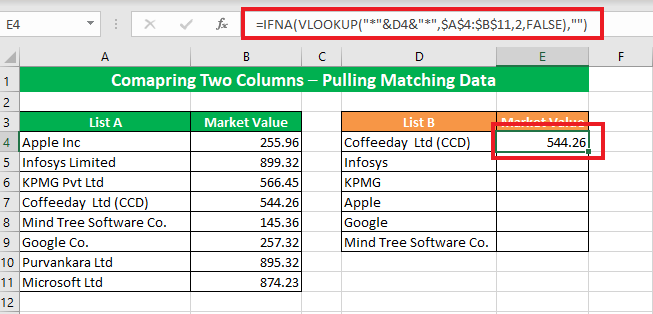
Step 2
Drag the cell handle and copy-paste the above formula into the remaining cell to get the partially matched data.
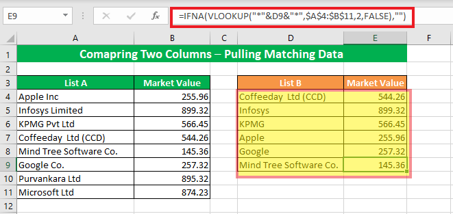
The above image shows how the VLOOKUP function finds data with partial matching using the asterisk (*) character. Cell D5 contains the value “Infosys,” whereas A5 contains the value” Infosys Limited.” Using the asterisk (*), VLOOKUP fetches those values even if they are not an absolute match.
Here’s a glance at how you can pull the matching data using the VLOOKUP function while comparing two columns.
Example Of Pulling Data by Comparing Two Columns
Since we are now well versed with the methods of comparison of two columns and pulling data in the third column using the VLOOKUP function, let us use the techniques altogether.
Consider the following example.
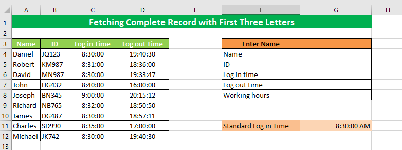
The above example shows employees’ records of their log-in and log-out time along with their company’s ID. Using this template, you can fetch the record of any employee by using the first three letters of their name.
Let us see how it works as below:
Step 1
Since the template works by using the first three letters of the employee’s name, the focus is placed on the Name column, i.e., G4.
To obtain results with only the first three letters of the employee’s name, the VLOOKUP function needs to work together with an asterisk. The first argument of the VLOOKUP function will look something like this:
=VLOOKUP (G3&”*”,
This argument is for the value of cell G3 with any number of letters on its right side. Insert the Function in the cell as:
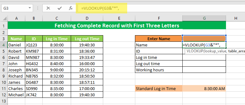
Step 2
For the table array, select the array range from A4 to D12 and turn it into an absolute reference.
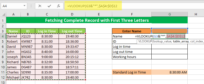
Step 3
Since we want to look up the Name column, which has the index 1 in the selected column array, the “Col_index_Num” is set to 1.
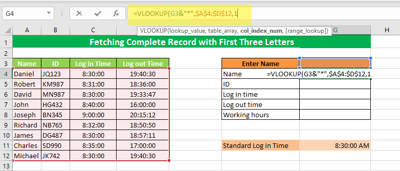
Step 4
For an exact match of the Name value, we put “False” as the last argument in the VLOOKUP function.
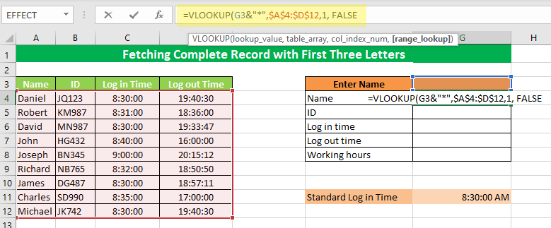
Step 5
Once done with the VLOOKUP function, close the bracket and press Enter. Entering the first three letters in cell G3, Excel gives back the following results.
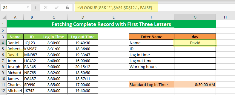
Step 6
For fetching the ID, let’s consider the value of G4 as the Look_up value. Since we are looking for an ID value that has Col_Ind_Num 2 in the selected table array, the Col_Ind argument is set to 2.
And for an exact match, we will add “FALSE” to the VLOOKUP function. The VLOOKUP function for fetching ID values will look like this:
=VLOOKUP (G4,$A$4:$D$12,2, FALSE)
Put the above formula in cell G5 and press Enter.
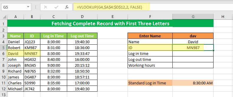
Step 7
For Log In time, we will use the same formula as we used for ID value; the only difference will be the Col_Ind number. It will be 3 for log-in time. The Function will look like this:
=VLOOKUP (G4,$A$4:$D$12,3, FALSE)
Put the above formula in cell G6 and press Enter.
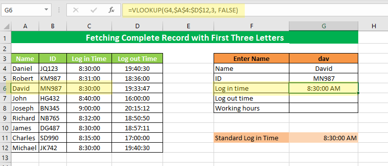
Step 8
For fetching Log out time, use the same formula with Col-Ind_Number as 4. It will look like this:
=VLOOKUP (G4,$A$4:$D$12,4, FALSE)
Put the formula in cell G7 and press Enter.

Step 9
The Working hours reflect the total time that an employee spends in the office. To calculate working hours, we will subtract the Log out time from the log-in time.
To do so, let’s bring to use the TEXT function. The syntax for the TEXT function for calculating working hours would take shape as follows.
=TEXT (G7-G6, “h:m”)
Put the above formula in cell G8 and press Enter.
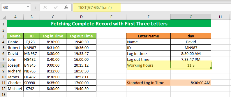
Step 10
The Conditional Formatting feature makes an appropriate choice to format the cell by comparing two cells.
If any employee logs in after the standard log-in time, the template should reflect it as follows.
Here is how the template works. It compares the given columns and fetches the required data using the VLOOKUP Function.
Not only that, it automatically calculates the working hours for each employee and indicates if any employee logged in late by changing the color of the cell.
Troubleshooting:
Comparing columns in Excel is a dynamic exercise – you can bring to your use a wide variety of functions, formulas, and tools to help the job.
However, if you get improper results while comparing two columns using the functions demonstrated above, do check for the following common problems.
-
-
#N/A Error
-
It is not an error in nature. Instead, it is a system message returned when you use the VLOOKUP Function to compare two columns for an exact match. In case of a mismatch, the VLOOKUP function returns the message #N/A.
To avoid such error messages, you can use the IFNA function to replace this error message with an empty cell instead.
The syntax for the IFNA function is as follows:
=IFNA (VLOOKUP (lookup_value, table_array, column_index_num, [range_lookup]),””)
Let’s recap on how to resolve this issue quickly.
-
-
#NAME? Error
-
If you get this error while using the VLOOKUP function, check out the VLOOKUP function syntax. One of the possible reasons for this error is the wrong spellings of “True” or “False” in the VLOOKUP function arguments.
-
-
#VALUE Error
-
Finding a #VALUE error indicates that you might have made some mistake while writing the VLOOKUP argument. Removing the syntax error can rid you of this error message.
Conclusion:
Excel provides a variety of methods and functions to compare two columns, including the use of a simple operator “=”, the EXACT Function, the IF Function, and the Conditional Formatting feature
Not limited to the above, you may use the VLOOKUP function for performing column comparisons in Excel. The VLOOKUP function is undoubtedly one of the most powerful functions of Excel to compare two columns and fetch matching or partially matching data into another column.
Practice the techniques discussed above to become an Excel whiz in no time. Happy Excel Exploring!
For more on Excel, check out our Using AI With Excel article here!