
Excel for Microsoft 365 Excel for Microsoft 365 for Mac Excel for the web Excel 2021 Excel 2021 for Mac Excel 2019 Excel 2019 for Mac Excel 2016 Excel 2016 for Mac Excel 2013 Excel 2010 Excel 2007 Excel for Mac 2011 Excel Starter 2010 More…Less
The CORREL function returns the correlation coefficient of two cell ranges. Use the correlation coefficient to determine the relationship between two properties. For example, you can examine the relationship between a location’s average temperature and the use of air conditioners.
Syntax
CORREL(array1, array2)
The CORREL function syntax has the following arguments:
-
array1 Required. A range of cell values.
-
array2 Required. A second range of cell values.
Remarks
-
If an array or reference argument contains text, logical values, or empty cells, those values are ignored; however, cells with zero values are included.
-
If array1 and array2 have a different number of data points, CORREL returns a #N/A error.
-
If either array1 or array2 is empty, or if s (the standard deviation) of their values equals zero, CORREL returns a #DIV/0! error.
-
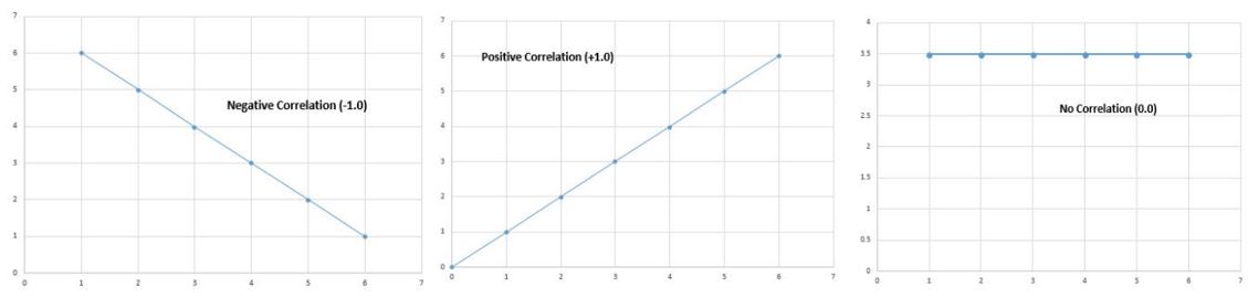
As much as the correlation coefficient is closer to +1 or -1, it indicates positive (+1) or negative (-1) correlation between the arrays. Positive correlation means that if the values in one array are increasing, the values in the other array increase as well. A correlation coefficient that is closer to 0, indicates no or weak correlation.
-
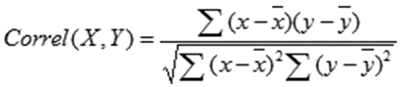
The equation for the correlation coefficient is:

where
are the sample means AVERAGE(array1) and AVERAGE(array2).

Example
The following example returns the correlation coefficient of the two data sets in columns A and B.

Need more help?
You can always ask an expert in the Excel Tech Community or get support in the Answers community.
Need more help?
Want more options?
Explore subscription benefits, browse training courses, learn how to secure your device, and more.
Communities help you ask and answer questions, give feedback, and hear from experts with rich knowledge.
What Is Correlation?
Correlation measures the linear relationship between two variables. By measuring and relating the variance of each variable, correlation gives an indication of the strength of the relationship.
To put it another way, correlation answers the question: How much does variable A (the independent variable) explain variable B (the dependent variable)?
Key Takeaways
- Correlation is the statistical linear correspondence of variation between two variables.
- In finance, correlation is used in several facets of analysis including the calculation of portfolio standard deviation.
- Computing correlation can be time-consuming, but software like Excel makes it easy to calculate.
Understanding Correlation
The Formula for Correlation
Correlation combines several important and related statistical concepts, namely, variance and standard deviation. Variance is the dispersion of a variable around the mean, and standard deviation is the square root of variance.
The formula is:
Since correlation wants to assess the linear relationship of two variables, what’s really required is to see what amount of covariance those two variables have, and to what extent that covariance is reflected by the standard deviations of each variable individually.
Common Mistakes With Correlation
The single most common mistake is assuming a correlation approaching +/- 1 is statistically significant. A reading approaching +/- 1 definitely increases the chances of actual statistical significance, but without further testing, it’s impossible to know.
The statistical testing of a correlation can get complicated for a number of reasons; it’s not at all straightforward. A critical assumption of correlation is that the variables are independent and that the relationship between them is linear. In theory, you would test these claims to determine if a correlation calculation is appropriate.
Remember, correlation between two variables does NOT imply that A caused B or vice versa.
The second most common mistake is forgetting to normalize the data into a common unit. If calculating a correlation on two betas, then the units are already normalized: beta itself is the unit. However, if you want to correlate stocks, it’s critical you normalize them into percent return, and not share price changes. This happens all too frequently, even among investment professionals.
For stock price correlation, you are essentially asking two questions: What is the return over a certain number of periods, and how does that return correlate to another security’s return over the same period?
This is also why correlating stock prices is difficult: Two securities might have a high correlation if the return is daily percent changes over the past 52 weeks, but a low correlation if the return is monthly changes over the past 52 weeks. Which one is «better»? There really is no perfect answer, and it depends on the purpose of the test.
Finding Correlation in Excel
There are several methods to calculate correlation in Excel. The simplest is to get two data sets side-by-side and use the built-in correlation formula:
This is a convenient way to calculate a correlation between just two data sets. But what if you want to create a correlation matrix across a range of data sets? To do this, you need to use Excel’s Data Analysis plugin. The plugin can be found in the Data tab, under Analyze.
Select the table of returns. In this case, our columns are titled, so we want to check the box «Labels in first row,» so Excel knows to treat these as titles. Then you can choose to output on the same sheet or on a new sheet.
Once you hit enter, the data is automatically made. You can add some text and conditional formatting to clean up the result.
Microsoft Excel lets you do more than simply create spreadsheets — you can also use the software to calculate key functions, such as the relationship between two variables. Known as the correlation coefficient, this metric is useful for measuring the impact of one operation on another to inform business operations.

Not confident in your Excel skills? No problem. Here’s how to calculate — and understand — the correlation coefficient in Excel.
![Download 10 Excel Templates for Marketers [Free Kit]](https://no-cache.hubspot.com/cta/default/53/9ff7a4fe-5293-496c-acca-566bc6e73f42.png)
What is Correlation?
Correlation measures the relationship between two variables. A correlation coefficient of 0 means that variables have no impact on one another — increases or decreases in one variable have no consistent effect on the other.
A correlation coefficient of +1 indicates a “perfect positive correlation”, which means that as variable X increases, variable Y increases at the same rate. A correlation value of -1, meanwhile, is a “perfect negative correlation”, which means that as variable X increases, variable Y decreases at the same rate. Correlation analysis may also return results anywhere between -1 and +1, which indicates that variables change at similar but not identical rates.
Correlation values can help businesses evaluate the impact of specific actions on other actions. For example, companies may find that as spending on social media marketing increases, so does customer engagement, indicating that more spending might make sense.
Or they may find that specific advertising campaigns result in a correlated decrease of customer engagement, in turn suggesting the need for a reevaluation of current efforts. The discovery that variables do not correlate can also be valuable; while common sense might suggest that a new function or feature in your product would correlate with increased engagement, it might have no measurable impact. Correlation analysis allows companies to view this relationship (or lack thereof) and make sound strategic decisions.
How to Calculate Correlation Coefficient in Excel
- Open Excel.
- Install the Analysis Toolpak.
- Select “Data” from the top bar menu.
- Select “Data Analysis” in the top right-hand corner.
- Select Correlation.
- Define your data range and output.
- Evaluate your correlation coefficient.
So how do you calculate the correction coefficient in Excel? Simple! Follow these steps:
1. Open Excel.
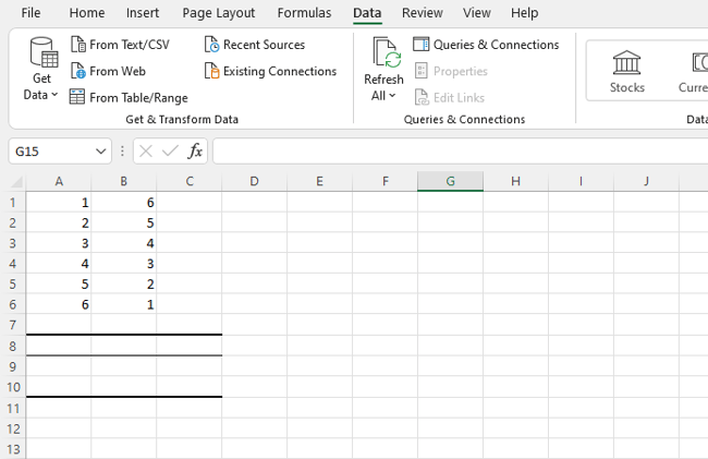
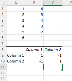
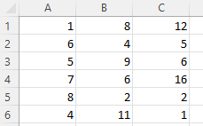
Step one: Open Excel and start a new worksheet for your correlated variable data. Enter the data points of your first variable in column A and your second variable in column B. You can add additional variables as well in columns C, D, E, etc. — Excel will provide a correlation coefficient for each one.
In the example below, we’ve entered six rows of data in column A and six in column B.
2. Install the Analysis Toolpak.
Next up? If you don’t have it, install the Excel Analysis Toolpak.
Select “File”, then “Options,” and you’ll see this screen:
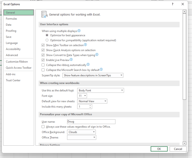
Select “Add-Ins” and then click on “Go”.
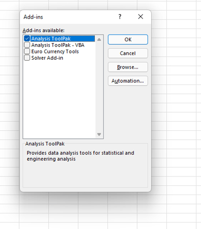
Now, check the box that says “Analysis ToolPak” and click “Ok”.
3. Select “Data” from the top bar menu.
Once you have the ToolPak installed, select “Data” from the top Excel bar menu. This provides you with a submenu that contains a variety of analysis options for your data.
4. Select “Data Analysis” in the top right-hand corner.
Now, look for “Data Analysis” in the top right-hand corner and click on it to get this screen:
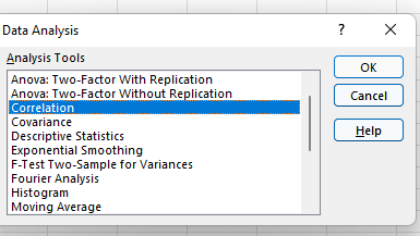
5. Select Correlation.
Select Correlation from the menu and click “OK.”
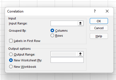
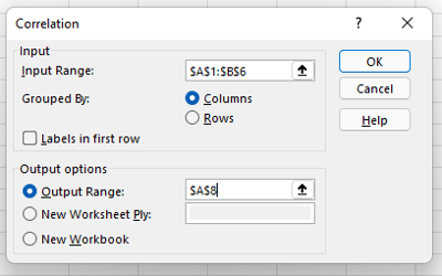
6. Define your data range and output.
Now define your data range and output. You can simply left-click and drag your cursor across the data you want to select, and it will auto-populate in the Correlation box. Finally, select an output range for your correlation data — we’ve chosen A8. Then, click “Ok”.
7. Evaluate your correlation coefficient.
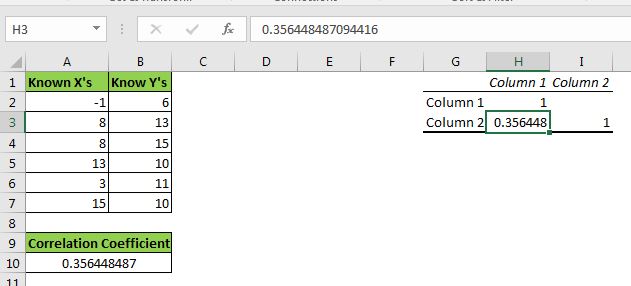
Your correlation results will now be displayed. In our example, values in column 1 and column 2 have a perfect negative correlation; as one goes up, the other goes down at the same rate.
The Excel Correlation Matrix
Excel correlation results are also known as an Excel correlation matrix. In the example above, our two columns of data produced a perfect correction matrix of 1 and -1. But what happens if we produce a correlation matrix with a less ideal data set?
Here’s our data:
And here’s the matrix:
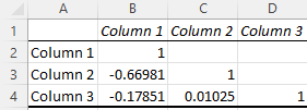
Cell C4 in the matrix gives us the correlation between Column 3 and Column 2, which is a very weak 0.01025, while Column 1 and Column 3 yield a stronger negative correlation of -0.17851. By far the strongest correlation, however, is between Column 1 and Column 2 at -0.66891.
So what does this mean in practice? Let’s say we were examining the impact of specific actions on the efficacy of a social media campaign, where Column 1 represents the number of visitors who click through on social advertisements and Columns 2 and 3 represent two different marketing taglines. The correlation matrix shows a strong negative correlation between Columns 1 and 2, which suggests that the Column 2 version of the tagline significantly decreased overall user engagement, while Column 3 drove only a slight decrease.
Regularly creating Excel matrices can help companies better understand the impact of one variable on another and determine what (if any) negative or positive effects may exist.
The Excel Correlation Formula
If you prefer to enter the correlation formula yourself, that’s also an option. Here’s what it looks like:
X and Y are your measurements, ∑ is the sum, and the X and Y with the bars over them indicate the mean value of the measurements. You would calculate it as follows:
- Calculate the sum of variable X minus the mean of X.
- Calculate the sum of variable Y minus the mean of Y.
- Multiply those two results and set that number aside (this is the first result).
- Square the sum of X minus the mean of X. Square the sum of Y minus the mean of Y. Multiply those two numbers.
- Take the square root (this is the second result).
- Divide the first result by the second result.
- You get the correlation coefficient.
Easy, right? Yes and no. While plugging in the numbers isn’t complicated, it’s often more trouble than it’s worth to create and manage this formula. The built-in Excel Toolpak is often a simpler (and faster) way to pinpoint coefficients and discover key relationships.
Correlation ≠ Not Causation
No article about correlation is complete without a mention that it does not equal causation. In other words, just because two variables rise or fall together doesn’t mean that one variable is the cause of the other variable’s increase or decrease.
Consider a few very strange examples.
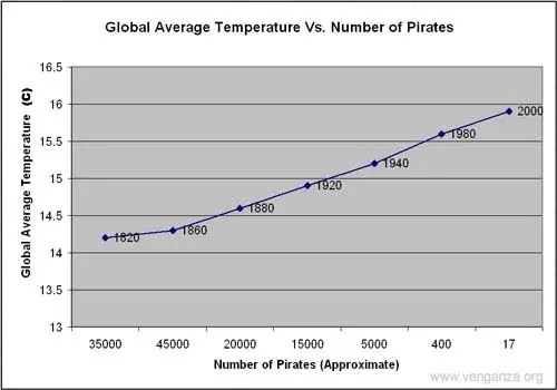
This image shows a near-perfect negative correlation between the number of pirates and the global average temperature — as pirates became more scarce, the average temperature increased.
The problem? While these two variables are correlated, there’s no causal link between the two; higher temperatures did not reduce the pirate population and fewer pirates did not cause global warming.
While correlation is a powerful tool, it only indicates the direction of increase or decrease between two variables — not the cause of this increase or decrease. To discover causal links, companies must increase or decrease one variable and observe the impact. For example, if correlation shows that customer engagement goes up with social media spending, it’s worth opting for a slight increase in spending followed by a measurement of results. If more spending leads directly to increased engagement, the link is both correlated and causal. If not, there may be one (or more) factors that underpin the increase of both variables.
Keeping Up with the Correlations
Excel correlations offer a solid starting point for marketing, sales, and spending strategy development, but they don’t tell the whole story. As a result, it’s worth using Excel’s built-in data analysis options to quickly evaluate the correlation between two variables and use this data as a jumping-off point for more in-depth analysis.

What is the Correlation Coefficient?
The correlation coefficient of a data set is a statistical number that tells how strongly two variables are related to each other. It can be said that it is the percentage of the relation between two variables (x and y). It can’t be greater than 100% and less than -100%.
The correlation coefficient falls between -1.0 and +1.0.
A negative correlation coefficient tells us that if one variable increases, other variable decreases. A correlation of -1.0 is a perfect negative correlation. This means that if x increases by 1 unit, y decreases by 1 unit.
A positive correlation coefficient tells us that if one variable’s value increases, other variable’s value also increases. This means that if x increases by 1 unit, y also increases by 1 unit.
The correlation of 0 says that there is no relation between two variables what so ever.
The Mathematical formula of Correlation Coefficient is:
=Coveriancexy/(Stdx*Stdy)
Coveriancexy is the covariance (sample or population) of data set.
Stdx= It is Standard Deviation (sample or population) of Xs.
Stdy= It is Standard Deviation (sample or population) of Ys.
How to Calculate the Correlation Coefficient in Excel?
If you need to calculate the correlation in excel, you do not need to use the mathematical formula. You can use these methods
- Calculating Correlation Coefficient using COREL function.
- Calculating Correlation Coefficient using Analysis Toolpak.
Let’s see an example to know how to calculate the correlation coefficient in excel.
Example of Calculation of correlation coefficient in excel
Here I have a sample data set. We have xs in range A2:A7 and ys in B2:B7.
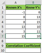
We need to calculate the correlation coefficient of xs and ys.
Using Excel CORREL Function
Syntax of the CORREL function:
array1: This is the first set of values (xs)
array2: It is the second set of values (ys).
Note: the array 1 and array 2 should be of the same size.
Let’s use the CORREL function to get the correlation coefficient. Write this formula in A10.
We get a correlation of 0.356448487 or 36% between x and y.
Using Excel Analysis Toolpak
To calculate correlation using analysis toolpak follow these steps:
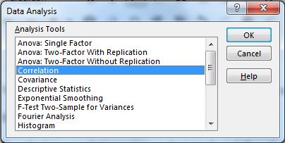
- Go to the Data tab on the ribbon. To the left most corner, you will find the data analysis option. Click on it. If you can’t see it, you first need to install the analysis toolpak.

- From the available options, select Correlation.
- Select the input range as A2:B7. Select the output range where you want to see your output.

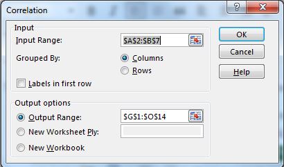
- Hit OK button. You have your correlation coefficient in the desired range. It is the exact same value as returned by the CORREL function.
 How correlation is being calculated?
To understand how we are getting this value, we need to find it manually. This will clear our doubts.
As we know the correlation coefficient is:
=Coveriancexy/(Stdx*Stdy)
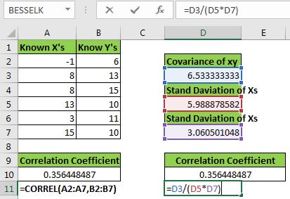
First, we need to calculate the covariance. We can use the COVERIACE.S function of excel to calculate it.
=COVARIANCE.S(A2:A7,B2:B7)
Next, let’s calculate the standard deviation of x and y using the STDEV.S function.
Now in cell D10, write this formula.
This is equivalent to =Covariancexy/(Stdx*Stdy). You can see that we get the exact same value as given by the CORREL function. Now you know how we have derived the correlation coefficient in excel.
Note: In the above example, we have used COVARIANCE.S (covariance of the sample) and STDEV.S (standard deviation of the sample). The correlation coefficient will be the same if you use COVARIANCE.P and STDEV.P. As long as they both are of the same category there will be no difference. If you use COVARIANCE.S (covariance of the sample) and STDEV.P (standard deviation of the population) then the result will be different and incorrect.
So yeah guys, this is how we can calculate correlation coefficient in excel. I hope this was explanatory enough to explain the correlation coefficient. You can now create your own correlation coefficient calculator in excel.
Related Articles:
Calculate INTERCEPT in Excel
Calculating SLOPE in Excel
Regressions in Excel
How to Create Standard Deviation Graph
Descriptive Statistics in Microsoft Excel 2016
How to Use Excel NORMDIST Function
Pareto Chart and Analysis
Popular Articles:
50 Excel Shortcut to Increase Your Productivity
The VLOOKUP Function in Excel
COUNTIF in Excel 2016
How to Use SUMIF Function in Excel
Correlation basically means a mutual connection between two or more sets of data. In statistics, bivariate data or two random variables are used to find the correlation between them. The correlation coefficient is generally the measurement of the correlation between the bivariate data which basically denotes how much two random variables are correlated with each other.
If the correlation coefficient is 0, the bivariate data are not correlated with each other.
If the correlation coefficient is -1 or +1, the bivariate data are strongly correlated with each other.
r=-1 denotes strong negative relationship and r=1 denotes strong positive relationship.
In general, if the correlation coefficient is close to -1 or +1 then we can say that the bivariate data are strongly correlated to each other.
The correlation coefficient is calculated using Pearson’s Correlation Coefficient which is given by :
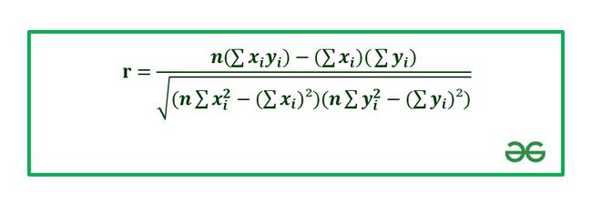
Correlation Coefficient
Where,
- r: Correlation coefficient.
-
*** QuickLaTeX cannot compile formula:


*** Error message:
Error: Nothing to show, formula is empty
: Values of the variable x.
- y_i: Values of the variable y.
- n: Number of samples taken in the data set.
- Numerator: Covariance of x and y.
- Denominator: Product of Standard Deviation of x and Standard Deviation of y.
In this article, we are going to see how to find correlation coefficients in Excel.
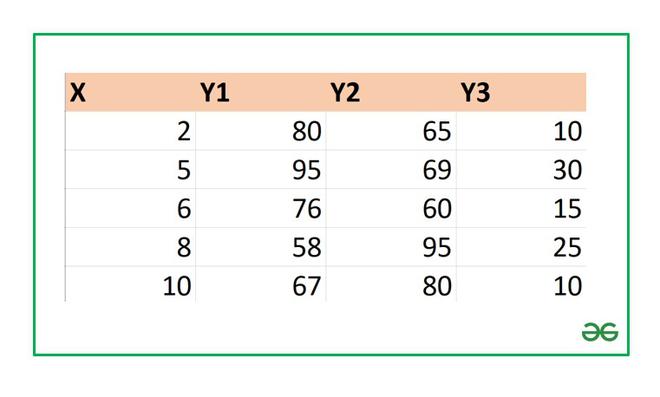
Example: Consider the following data set :
Finding the Correlation Coefficient in Excel:
1. Using CORREL function
In Excel to find the correlation coefficient use the formula :
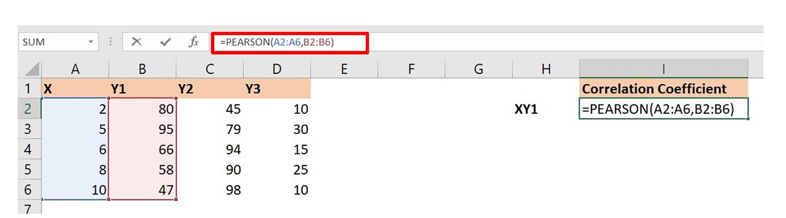
=CORREL(array1,array2)
array1 : array of variable x
array2: array of variable y

To insert array1 and array2 just select the cell range for both.
1. Let’s find the correlation coefficient for the variables and X and Y1.
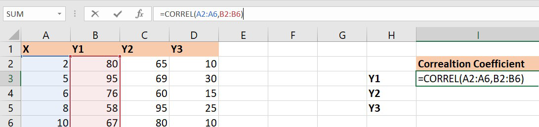
Correlation coefficient of x and y1
array1 : Set of values of X. The cell range is from A2 to A6.
array2 : Set of values of Y1. The cell range is from B2 to B6.
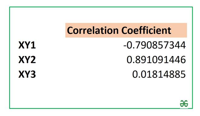
Similarly, you can find the correlation coefficients for (X , Y2) and (X , Y3) using the Excel formula. Finally, the correlation coefficients are as follows :
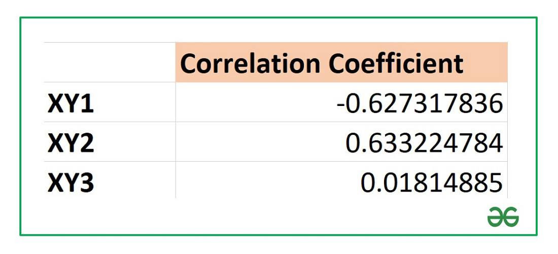
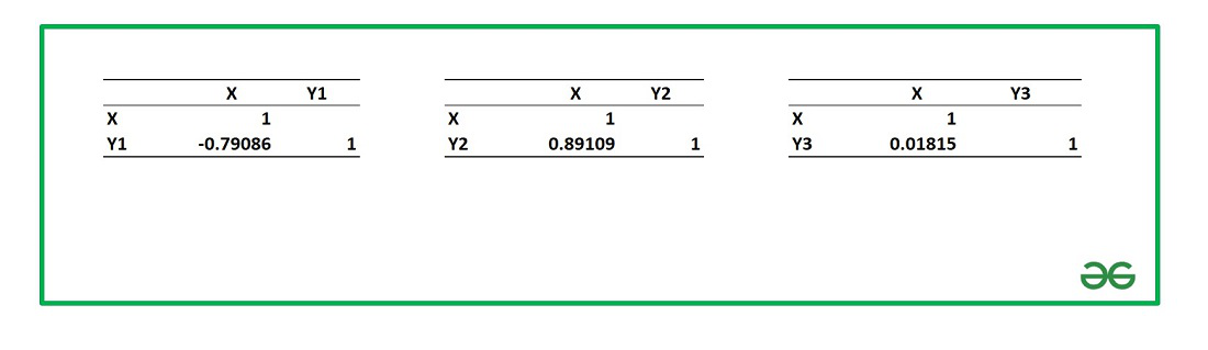
From the above table we can infer that :
X and Y1 have negative correlation coefficient.
X and Y2 have positive correlation coefficient.
X and Y3 are not correlated as the correlation coefficient is almost zero.
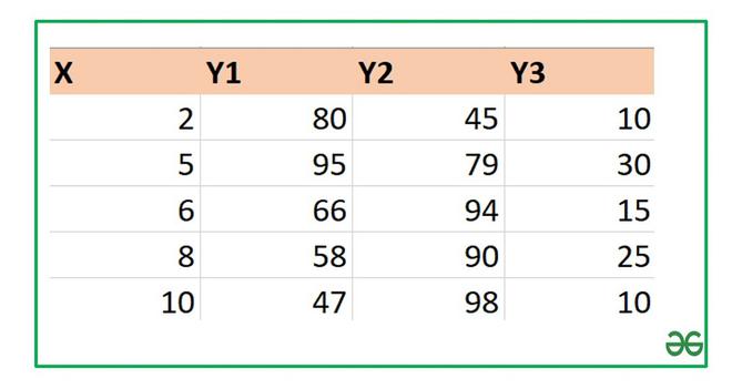
Example: Now, let’s proceed to the further two methods using a new data set. Consider the following data set :
Using Data Analysis
We can also analyze the given dataset and calculate the correlation coefficient: To do so follow the below steps:
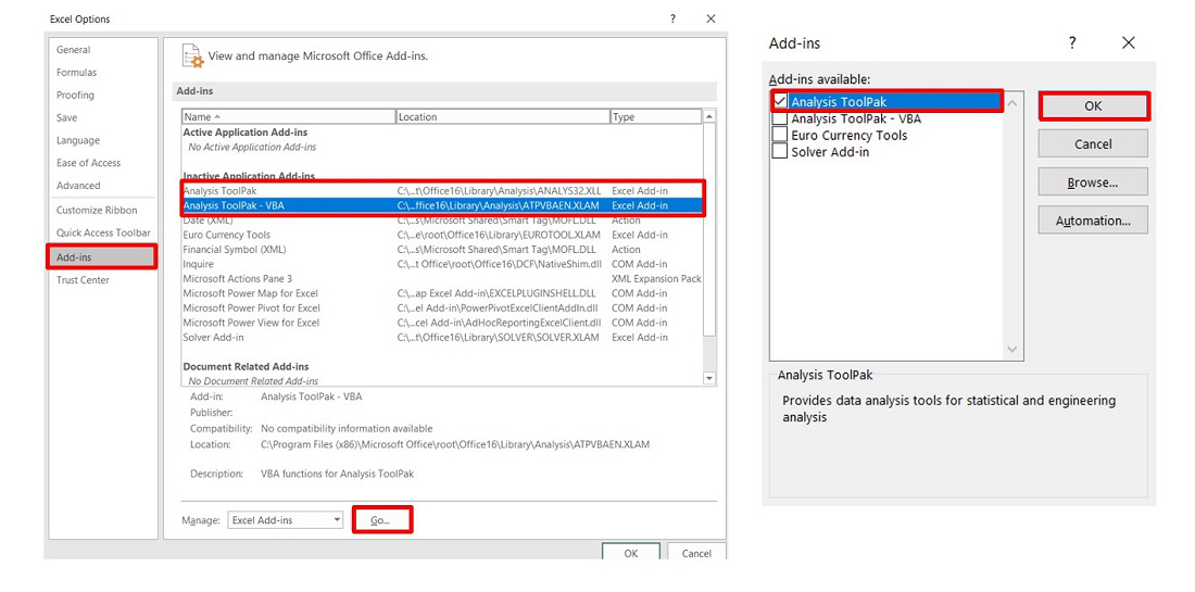
Step 1: First you need to enable Data Analysis ToolPak in Excel. To enable :
- Go to File tab in the top left corner of the Excel window and choose Options.
- The Excel Options dialog box opens. Now go to the Add-Ins option and in the Manage select Excel Add-ins from the drop down.
- Click on Go button.
- The Add-ins dialog box opens. In this check the option Analysis ToolPak.
- Click OK!

Data Analysis tab added
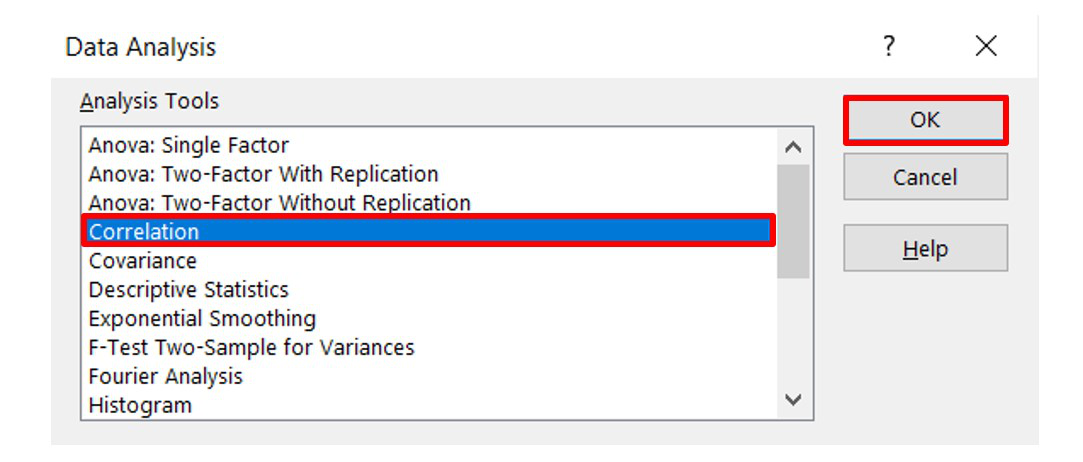
Step 2: Now click on Data followed by Data Analysis. A dialog box will appear.
Step 3: In the dialog box select Correlation from the list of options. Click OK!
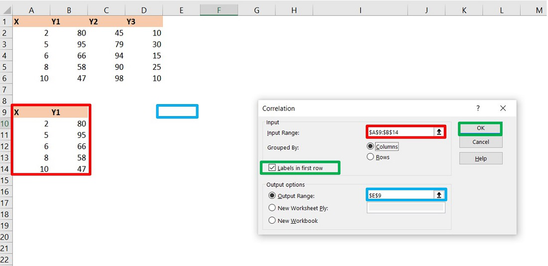
Step 4: The Correlation menu will appear.
Step 5: In this menu first provide the Input Range. The input range is the cell range of X and Y1 columns as highlighted in the picture below.
Step 6: Also, supply the Output Range as the cell number where you want to display the result. By default, the output will appear in the new Excel sheet in case if you don’t provide any Output Range.
Step 7: Check the Labels in first-row option if you have labels in the dataset. In our case column 1 has label X and column 2 has label Y1.
Step 8: Click OK.
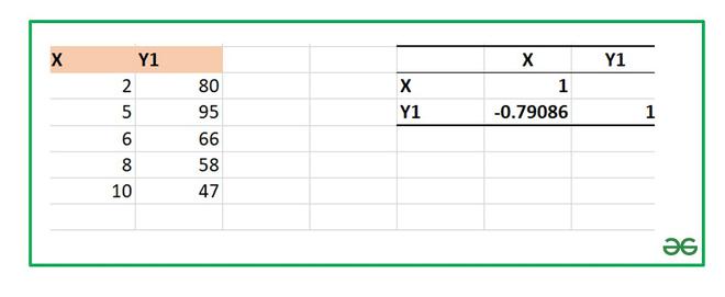
Step 9: The Data Analysis table is now ready. Here, you can see the correlation coefficient between X and Y1 in the analysis table.
Similarly, you can find correlation coefficients of XY2 and that of XY3. Finally, all the correlation coefficients are :
Using PEARSON Function
It is exactly similar to the CORREL function which we have discussed in the above section. The syntax for PEARSON function is :
=PEARSON(array1,array2)
array1 : array of variable x
array2: array of variable y

To insert array1 and array2 just select the cell range for both.
Let’s find the correlation coefficient for X and Y1 in the data set of Example 2 using PEARSON function.
The formula will return the correlation coefficient of X and Y1. Similarly, you can do for others.
The final correlation coefficients are :
One way to quantify the relationship between two variables is to use the Pearson correlation coefficient which is a measure of the linear association between two variables.
It always takes on a value between -1 and 1 where:
- -1 indicates a perfectly negative linear correlation between two variables
- 0 indicates no linear correlation between two variables
- 1 indicates a perfectly positive linear correlation between two variables
To determine if a correlation coefficient is statistically significant you can perform a correlation test, which involves calculating a t-score and a corresponding p-value.
The formula to calculate the t-score is:
t = r√(n-2) / (1-r2)
where:
- r: Correlation coefficient
- n: The sample size
The p-value is calculated as the corresponding two-sided p-value for the t-distribution with n-2 degrees of freedom.
The following step-by-step example shows how to perform a correlation test in Excel.
Step 1: Enter the Data
First, let’s enter some data values for two variables in Excel:

Step 2: Calculate the Correlation Coefficient
Next, we can use the CORREL() function to calculate the correlation coefficient between the two variables:

The correlation coefficient between the two variables turns out to be 0.803702.
This is a highly positive correlation coefficient, but to determine if it’s statistically significant we need to calculate the corresponding t-score and p-value.
Step 3: Calculate the Test Statistic and P-Value
Next, we can use the following formulas to calculate the test statistic and the corresponding p-value:

The test statistic turns out to be 4.27124 and the corresponding p-value is 0.001634.
Since this p-value is less than .05, we have sufficient evidence to say that the correlation between the two variables is statistically significant.
Additional Resources
How to Create a Correlation Matrix in Excel
How to Calculate Spearman Rank Correlation in Excel
How to Calculate Rolling Correlation in Excel