Can excel be used for statistics

Using Excel for Statistical Analysis

MS Excel is one of the most commonly used tools for data analysis. The convenience of use and cost are two very important reasons why most data professionals prefer using Excel for statistical data analysis. However, using Excel for statistical analysis requires clarity of thought, data analysis knowledge, and strong decision-making skills.

Whether you are performing statistical analysis using Excel 2010 or Excel 2013, you need to have a clear understanding of charts and pivot tables. Most data analysts using Excel for statistical analysis depend largely on these two Excel features. Having knowledge of the essential statistics for data analysis using Excel answers is a plus.

Remember to install Data Analysis ToolPak if you are using Excel for statistical data analysis. In this discussion, we explain in detail the essential statistics for data analysis using Excel and how to perform descriptive analysis using Excel.

In this blog, I have tried to explore the functionalities of MS-Excel as a potential tool for statistical analysis and suggested some simple tricks and techniques that will save both time and energy.

Using Excel for Statistical Analysis: Pivot Tables

A PivotTable is an Excel tool for summarizing a list into a simple format. It helps you analyze all the data in your worksheet so as to make better business decisions. Excel can help you by recommending, and then, automatically creating PivotTables, which are a great way to summarize, analyze, explore, and present your data.

A pivot table may be used as an interactive data summarization tool to automatically condense large datasets into a separate, concise table. You can use it to create an informative summary of a large dataset or make regional comparisons between brand sales.

You can create PivotTables from lists, as you define which fields should be arranged in columns, which fields should become rows, and what data you wish to summarize.

Using Excel for Statistical Analysis: Descriptive Statistics

Descriptive Statistics tool in the Data Analysis add-in can be used on an existing data set to get up to 16 different descriptive statistics, without having to enter a single function on the worksheet. Descriptive Statistics gives you a general idea of trends in your data including:

• The mean, mode, median and range
• Variance and standard deviation
• Skewness
• Sample Variance
• Kurtosis and Skewness
• Count, maximum and minimum

Descriptive Statistics is useful because it allows you to take a large amount of data and summarize it. For example, you may want to represent the incomes of a community. Instead of showing it on an excel, you may summarize it, it becomes useful: an average wage, or a median income, is much easier to understand and then analyze the data.

You can find descriptive analysis by going to Excel→ Data→ Data Analysis → Descriptive statistics. It is the most basic set of analysis that can be performed on any data set.

Using Excel for Statistical Analysis: ANOVA (Analysis of Variance)

Analysis of variance (ANOVA) is a statistical technique that is used to check if the means of two or more groups are significantly different from each other. ANOVA checks the impact of one or more factors by comparing the means of different samples.

ANOVA method in Excel shows whether the mean of two or more data set is significantly different from each other or not. In other words, ANOVA analyses two or more groups simultaneously and finds out whether any relationship is there among the groups of data set or not.

For example, you may use ANOVA if you want to analyze the traffic of three different cities and find out which one is more efficient in handling the traffic (or if there are no significant differences among the traffic).

You will find three types of ANOVA in Excel:

• ANOVA single factor
• ANOVA two factor with replication
• ANOVA two factor without replication

If you have three groups of datasets and want to check whether there is any significant difference between these groups or not, you can use ANOVA single factor. If the P-value in the ANOVA summary table is greater than 0.05, you can say that there is a significant difference between the groups.

Using Excel for Statistical Analysis: Moving Average

Moving Average, another great tool for those using Excel for statistical analysis, is ideal for time series data such as stock price, weather report, attendance in class, etc. Moving Average is used extensively in stock price as a technical indicator. If you want to predict the stock price of today, the last ten days’ data would be more relevant than the last 1 year.

You may, simply plot the moving average of the stock having a 10-day period and then predict the estimated price. The same rule may be applied for predicting the temperature of a city. The recent temperature of a city can be calculated by taking the average of the last few weeks rather than the last few months.

Using Excel for Statistical Analysis: Rank and Percentile

The Rank and Percentile, another popular Excel features used for data analysis, is useful for finding the rank of all the values in a list. The best part of using the Rank and Percentile feature is that the percentile is also added to the output table.

The percentile is a percentage that indicates the proportion of the list which is below a given number. It calculates the ranking and percentile in the data set. For example, if you are managing a business of several products and want to find out which product is contributing to a higher revenue, you can use this rank method in Excel.

In the left table, we have our data on the revenues of different products. And we want to rank this data of products based on their revenue. With the help of rank and percentile, we can get the table shown on the right. You can observe that now the data is sorted and respective rank is also marked with each data.

Percentile shows the category in which the data belongs, such as the top 50%, top 30%, etc. In the summary table, the rank of product 7 is 4. As the total number of data is 7, we can easily say that it belongs to the top 50% of the data.

Using Excel for Statistical Analysis: Regression

Regression is one of the best features in Excel. It is widely used for using Excel for statistical data analysis. Regression is a process of establishing a relationship among many variables; to establish a relationship between dependent variables and independent variables.

Regression is great for use for using Excel for statistical data analysis. You, may, for example, want to see if there is an increase in the revenue of the product, which is not due to the increase in the advertisement.

If you performing statistical analysis using Excel 2010, Regression Analysis is the best way of mathematically sorting out which of those variables does indeed have an impact. It answers the questions: Which factors matter most? Which can we ignore? How do those factors interact with each other? And, perhaps most importantly, how certain are we about all of these factors?

These factors are more commonly known as variables. You may have your dependent or independent variables. In order to conduct a regression analysis, you gather the data on the variables in question.

You may take all of your monthly sales numbers, the past five years and any data on the independent variables you may find useful. You may, for example, find out the average monthly rainfall for the past five years as well.

Using Excel for Statistical Analysis: Random Number Generator

If you are using Excel for statistical data analysis, on a regular basis, Random Number Generator must be your top choice for generating a series of random numbers. This simple function in Excel gives you more flexibility in the random number generation process. It gives you more control over the generated data.

A random number is one that is drawn from a set of possible values, each of which is equally probable. In statistics, this is called a uniform distribution, because the distribution of probabilities for each number is uniform (i.e., the same) across the range of possible values.

For example, a good (unloaded) die has the probability 1/6 of rolling a one, 1/6 of rolling a two and so on. Hence, the probability of each of the six numbers coming up is exactly the same, so we say any roll of our die has a uniform distribution.

When discussing a sequence of random numbers, each number drawn must be statistically independent of the others. This means that drawing one value doesn’t make that value less likely to occur again. This is exactly the case with our unloaded die: If you roll a six, that doesn’t mean the chance of rolling another six changes.

Two very essential statistics for data analysis using Excel:

• The function RANDBETWEEN returns a random integer number
• The function RAND () returns a random real number of a uniform distribution. It will be less than 1 and greater than or equal to 0.

Using Excel for Statistical Analysis: Sampling

Sampling is one of the most readily preferred Excel tools if you are using Excel for statistical data analysis. This option is used for creating samples from a huge population. You can randomly select data from the dataset or select every nth item from the set.

For example, if you may want to measure the effectiveness of female call center employee in a call center, you can use this tool to randomly select few data every month and listen to their recorded calls and give a rating based on the selected call.

Sampling Methods:

If you are using statistical analysis using Excel 2010, you can make use of two sampling methods in Excel for retrieving or identifying items in your data set:

• Periodic: In this case, you specify the Period n at which you want sampling to take place. The nth value in the input range and every nth value thereafter is copied to the output column. Sampling stops when the end of the input range is reached.
• Random: In this case, you specify the Random Number of Samples. This number of values is drawn from random positions in the input range. A value can be selected more than once. (I.e. sampling is with replacement).

The data science field is booming to such an extent that our earlier analysis of employment reported that there are currently more than 97,000 job openings in India for analytics and information science. Thus, building a career in Data Science is quite in trend these days as the Data Science domain offers lucrative career options.

Excel is one of the most dynamic and intriguing tools for statistical analysis. We have discussed a few features. Play around with Excel to know more about other tools and techniques. You may also look for essential statistics for data analysis using Excel answers.

We offer one of the best-known courses in the Certified Data Analytics Course. The course enables you to learn tools such as Advanced Excel, PowerBI, and SQL.  The live projects and intensive training program also empower you to come up with solutions for real-life problems.

Microsoft Excel can do statistics! You can calculate percentages, averages, standard deviation, standard error, and student’s T-tests.

Despite not being as powerful as software specifically for statistics, Excel is actually quite adept at running basic calculations, even without add-ins (though there are some add-ins that make it even better).

You probably know that it can do arithmetic, but did you know that it can also quickly get percentage change, averages, standard deviation from samples and populations, standard error, and student’s T-tests?

Excel has a lot of statistical power if you know how to use it. We’ll take a look at some of the most basic statistical calculations below. Let’s get started!

How to Calculate Percentage in Excel

Calculating percentages in Excel is as simple as it is anywhere else: just divide two numbers and multiply by 100. Let’s say that we’re calculating the percentage of 347 out of 521.

Simply divide 347 by 521 using the syntax =347/521. (If you’re not familiar with Excel, the equals sign tells Excel that you want it to calculate something. Just enter the equation after that and hit Enter to run the calculation.)

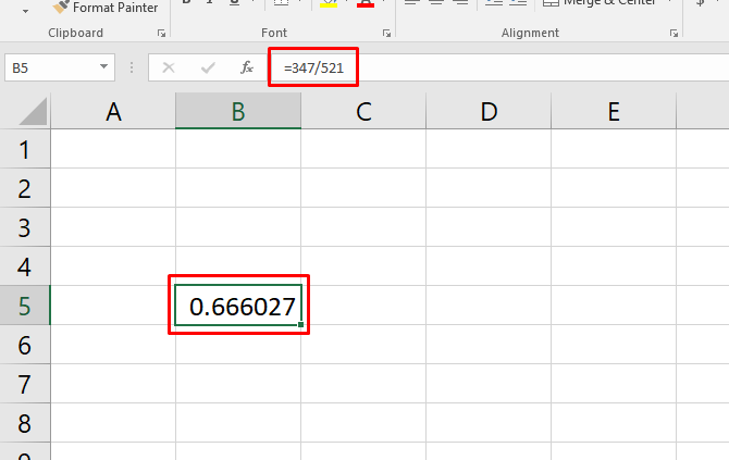
You now have a decimal value (in this case, .67). To convert it into a percentage, hit Ctrl + Shift + 5 on your keyboard (this is a very useful Excel keyboard shortcut to add to your arsenal).

You can also change the cell format the long way by right-clicking the cell, selecting Format Cells, choosing Percentage, and clicking OK.

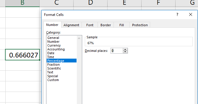
Keep in mind that changing the format of the cell takes care of the «multiply by 100» step. If you multiply by 100 and then change the format to percentage, you’ll get another multiplication (and the wrong number).

Tip: Learn how to create dropdown lists for Excel cells.

How to Calculate Percentage Increase in Excel

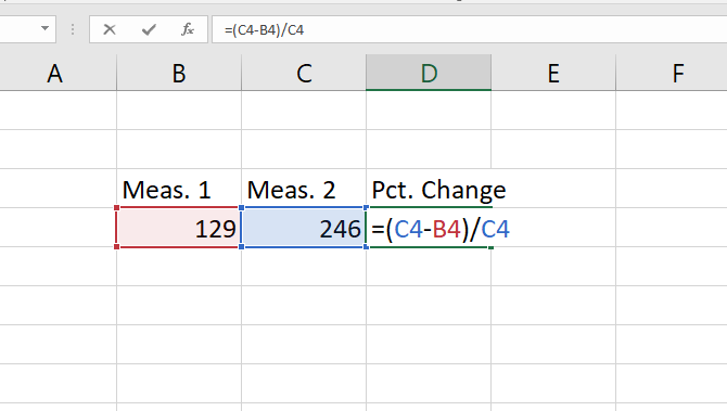
Calculating the percentage increase is similar. Let’s say our first measurement is 129, and our second is 246. What’s the percentage increase?

To start, you’ll need to find the raw increase, so subtract the initial value from the second value. In our case, we’ll use =246-129 to get a result of 117.

Now, take the resulting value (the raw change) and divide it by the original measurement. In our case, that’s =117/129. That gives us a decimal change of .906. You can also get all of this information in a single formula like this:

Use the same process as above to convert this to a percentage, and you’ll see that we have a 91 percent change. Do a quick check: 117 is almost equal to 129, so this makes sense. If we would have calculated a change value of 129, the percentage change would have been 100 percent.

How to Calculate Mean (Average) in Excel

One of Excel’s most useful built-in functions calculates the mean (average) of a set of numbers. If you haven’t used an Excel function before, you’ll be impressed at how easy it is. Just type in the name of the function, select the cells you want to apply it to, and hit Enter.

In our example here, we have a series of measurements that we need the average of. We’ll click into a new cell and type =AVERAGE(, then use the mouse to select the relevant cells (you can also type in the cell range if you’d like). Close the parentheses with a ) and you’ll have a formula that looks like this: =AVERAGE(B4:B16)

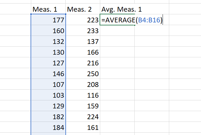
Hit Enter, and you’ll get the average! That’s all there is to it.

You can also use Excel to calculate the weighted average.

How to Calculate a Student’s T-Test in Excel

A Student’s t-test calculates the chances that two samples came from the same population. A lesson in statistics is beyond this article, but you can read up more on the different types of Student’s t-tests with these free resources for learning statistics (Statistics Hell is my personal favorite).

In short, though, the P-value derived from a Student’s t-test will tell you whether there’s a significant difference between two sets of numbers.

Let’s say you have two measurements from the same group and you want to see if they’re different. Say you weighed a group of participants, had them go through personal training, and then weighed them again. This is called a paired t-test, and we’ll start with this.

Excel’s T.TEST function is what you need here. The syntax looks like this:

 =T.TEST(array1, array2, tails, type) 

array1 and array2 are the groups of numbers you want to compare. The tails argument should be set to «1» for a one-tailed test and «2» for a two-tailed test.

The type argument can be set to «1,» «2,» or «3.» We’ll set it to «1» for this example because that’s how we tell Excel we’re doing a paired t-test.

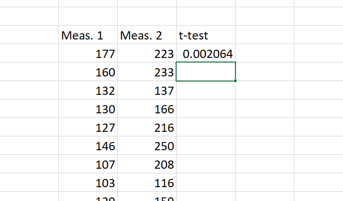
Here’s what the formula will look like for our example:

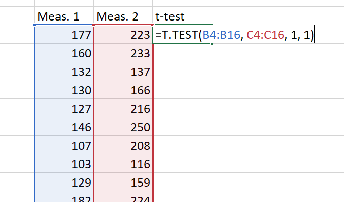
Now we just hit Enter to get our result! It’s important to remember that this result is the P value. In most fields, a P value of less than .05 indicates a significant result.

The basics of the test are the same for all three types. As mentioned, a «1» in the type field creates a paired t-test. A «2» runs a two-sample test with equal variance, and a «3» runs a two-sample test with unequal variance. (When using the latter, Excel runs a Welch’s t-test.)

How to Calculate Standard Deviation in Excel

Calculating standard deviation in Excel is just as easy as calculating the average. This time, you’ll use the STDEV.S or STDEV.P functions, though.

STDEV.S should be used when your data is a sample of a population. STDEV.P, on the other hand, works when you’re calculating the standard deviation for an entire population. Both of these functions ignore text and logical values (if you want to include those, you’ll need STDEVA or STDEVPA).

To determine the standard deviation for a set, just type =STDEV.S() or =STDEV.P() and insert the range of numbers into the parentheses. You can click-and-drag or type the range.

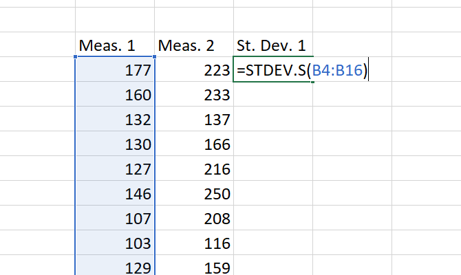
At the end, you’ll have a number: that’s your standard deviation.

How to Calculate Standard Error in Excel

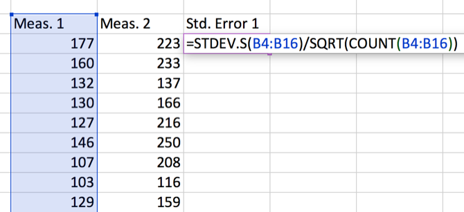
Standard error is closely related to standard deviation. And while Excel doesn’t have a function that will calculate it, you can quickly find it with minimal effort.

To find the standard error, divide the standard deviation by the square root of n, the number of values in your dataset. You can get this information with a single formula:

 =STDEV.S(array1)/SQRT(COUNT(array1)) 

If you’re using text or logical values in your array, you’ll need to use COUNTA instead.

Here’s how we’d calculate the standard error with our dataset:

Using Excel for Statistics: Not Great but Workable

Can you use Excel for statistics and complex calculations? Yes. Will it work as well as dedicated statistical software like SPSS or SAS? No. But you can still calculate percentages, averages, standard deviations, and even t-tests.

When you need a quick calculation, and your data is in Excel, you don’t need to import it into different software. And that’ll save you time. You can also use Excel’s Goal Seek feature to solve equations even faster.

Don’t forget to put your data into aesthetically pleasing and informative graphs before you show it to your colleagues! And it would also help to master IF statements in Excel.

Descriptive statistics with excel is a popular way to describe your data. It makes the tons of formula became easier just by simple click and drop.

Years ago, I do the formula one by one and find the statistic value that I need. It is really uncomfortable, is not it?

You have to remember the correct formula of your data and choose the right formula because perhaps there is more than one similar formula for one statistic value.

Look at he picture I present below. This is what you will using descriptive statistics with excel by typing the formula one by one

There are 7 formulas that excel provide to you to generate the variance of your data. My question is, which one will you use?

Still, writing one by one formula to summarize the statistic value that you need? Well, keep reading!

Microsoft Excel is a phenomenal software developed by Microsoft helping Billions of human to solve their problems. Excel helps us to makes almost our calculation problem easier included statistics.

Why using descriptive statistics in excel?

If you are wondering why you should Microsoft Excel to process your statistical data, let me tell you these interesting facts!

1. The user interface is so friendly

Yes, Microsoft Excel interface is so friendly so almost every user could use it without any meaningful problem. You may use it through simple steps and clicks to produce the output that you want.

2. No coding needed

Usually, almost all statistical software needs to code the form. But, Excel does not require you to code anything. You just need to know the simple formula or use the toolbar that will help you to finish the job.

3. Easy to interpret

The output is served simply so we may see it and understand what the output is. If you did not strong statistical basics, do not worry. It’s just basic formula which you may learn in your study.

Before using Microsoft Excel to process your data, you must activate the data analysis toolpak to makes your job easier.

Follow these simple steps!

1. Activate the data analysis toolpak, go to file >> options

2. Choose add ins >> analysis toolpak

3. Ok

Now, you will have the tools that you need to make your works easier and faster. By using this toolpak, you do not have to input every single formula that you need. Now, let’s calculate the descriptive statistics in excel

Already have your data set? Let’s do the analysis. Here is the steps!

1. Go to Data >> data analysis

2. You’ll see many statistical options there, choose descriptive statistics >> ok

3. In the popup window, you have several fields that you have to fill

• Input range: block the data you want to analyze
• Grouped by: whether the data is grouped in columns or rows
• Labels in the first row: if the blocked data has labels in the first row, check this
• Output options: where the output will be displayed
• Summary statistics: if you want to do descriptive statistics analysis
• The confidence level for mean: if you want to show confidence level for mean
• Kth largest: if you want to show the data in “k”th largest
• Kth smallest: if you want to show the data in “k”th smallest

4. Click Ok

5. See the magic happens!

Interpretation of Descriptive Statistics Output in Excel

1. Mean = 7,434. In average, there are 7,434 poor people in these 12 areas

2. Standard error = 468.412. This value indicates that the sample we chose has a fairly high distribution of the population mean.

3. Median = 7,575. This value indicates that the middle numbers of poor people based on the sample we use are 7,575 people.

4. Mode = 8000. This value shows that the most number of poor people based on the sample we have is 8000 people.

5. Standard deviation = 1622. This value indicates that the sample values ​​that we use are spread far enough from the mean value.

6. Kurtosis = -0.68485. Because the value of kurtosis is smaller than 3, we can conclude that the sample used is platicurtic distribution (tends to be flat).

7. Skewness = -0.12018. Because the skewness value is smaller than zero, we can conclude that the data tends to be left inclined or left skewed.

8. Range = 5100. This value indicates that the difference between the regions with the highest number of poor people and the lowest number of poor people is 5100 people.

9. Minimum = 4900. This value shows the lowest number of poor people is 4900 people in the L area.

10. Maximum = 10,000. This value shows that the highest number of poor people is 10,000 people in J area.

11. Sum = 89,210. This value indicates that the total number of poor people based on the data used was 89,210 people.

12. Count = 12. This value indicates the amount of data used is 12.

13. Confidence level = 1030,968. It’s quite difficult to understand, right? Okay, keep reading.

Confidence interval means we will predict a value in the form of a range. In this case, we need upper values ​​and lower values.

In the descriptive statistics feature in Microsoft Excel, they only provide one value, and this figure is very far from the mean.

The confidence level value that appears is a value that can be used to get the upper and lower limits of the confidence interval you are using.

If you want to get the upper limit, you simply add an average to the value of the confidence level. The following calculations. Check the picture below!

If you want to get a lower bound value, you can simply reduce the average value with that confidence level. Consider the following picture.

Now, let’s make the interpretation of this value!

With a confidence level of 95 percent, the average number of poor people in the 12 regions is 6,403 to 8,465 people.

The Disadvantage of Using Excel For Descriptive Statistics

1. The formula is limited

Although the formula is super easy just by drag and click, the numbers of excel formula in the statistical process are limited.

Excel provided not much formula so the user can use to do data processing. But, Excel is the best tool to study statistical computing if you want to be advanced in the future.

2. It is only for numerical data

It’s sad but if you are using categorical or non-numeric data, probably excel is not for your research. Excel only read the data in numeric format. Even you transform it into numerical form, it’s quite difficult to read the output.

3. It is only for single variable analysis

Conclusion

Overall, the steps of using descriptive statistics in excel are:

1. Prepare the data set.

2. Activate analysis toolpak add-ins add options menu.

3. Choose the descriptive statistics at the data analysis menu.

4. Check the statistic value that you want to generate.

5. Click Ok.

6. Do not forget to make the output interpretation.

If you want to do more advanced analysis by software, I recommend you to check the descriptive statistics on spss article. You will find an easier way to produce the descriptive statistics even for the numerical or categorical data set.