
Enter data manually in worksheet cells
Excel for Microsoft 365 Excel 2021 Excel 2019 Excel 2016 Excel 2013 Excel 2010 Excel 2007 More…Less
You have several options when you want to enter data manually in Excel. You can enter data in one cell, in several cells at the same time, or on more than one worksheet at once. The data that you enter can be numbers, text, dates, or times. You can format the data in a variety of ways. And, there are several settings that you can adjust to make data entry easier for you.
This topic does not explain how to use a data form to enter data in worksheet. For more information about working with data forms, see Add, edit, find, and delete rows by using a data form.
Important: If you can’t enter or edit data in a worksheet, it might have been protected by you or someone else to prevent data from being changed accidentally. On a protected worksheet, you can select cells to view the data, but you won’t be able to type information in cells that are locked. In most cases, you should not remove the protection from a worksheet unless you have permission to do so from the person who created it. To unprotect a worksheet, click Unprotect Sheet in the Changes group on the Review tab. If a password was set when the worksheet protection was applied, you must first type that password to unprotect the worksheet.
-
On the worksheet, click a cell.
-
Type the numbers or text that you want to enter, and then press ENTER or TAB.
To enter data on a new line within a cell, enter a line break by pressing ALT+ENTER.
-
On the File tab, click Options.
In Excel 2007 only: Click the Microsoft Office Button
 , and then click Excel Options.
 -
Click Advanced, and then under Editing options, select the Automatically insert a decimal point check box.
-
In the Places box, enter a positive number for digits to the right of the decimal point or a negative number for digits to the left of the decimal point.
For example, if you enter 3 in the Places box and then type 2834 in a cell, the value will appear as 2.834. If you enter -3 in the Places box and then type 283, the value will be 283000.
-
On the worksheet, click a cell, and then enter the number that you want.
Data that you typed in cells before selecting the Fixed decimal option is not affected.
To temporarily override the Fixed decimal option, type a decimal point when you enter the number.
 , and then click Excel Options.
-
On the worksheet, click a cell.
-
Type a date or time as follows:
-
To enter a date, use a slash mark or a hyphen to separate the parts of a date; for example, type 9/5/2002 or 5-Sep-2002.
-
To enter a time that is based on the 12-hour clock, enter the time followed by a space, and then type a or p after the time; for example, 9:00 p. Otherwise, Excel enters the time as AM.
To enter the current date and time, press Ctrl+Shift+; (semicolon).
-
-
To enter a date or time that stays current when you reopen a worksheet, you can use the TODAY and NOW functions.
-
When you enter a date or a time in a cell, it appears either in the default date or time format for your computer or in the format that was applied to the cell before you entered the date or time. The default date or time format is based on the date and time settings in the Regional and Language Options dialog box (Control Panel, Clock, Language, and Region). If these settings on your computer have been changed, the dates and times in your workbooks that have not been formatted by using the Format Cells command are displayed according to those settings.
-
To apply the default date or time format, click the cell that contains the date or time value, and then press Ctrl+Shift+# or Ctrl+Shift+@.
-
Select the cells into which you want to enter the same data. The cells do not have to be adjacent.
-
In the active cell, type the data, and then press Ctrl+Enter.
You can also enter the same data into several cells by using the fill handle
to automatically fill data in worksheet cells.For more information, see the article Fill data automatically in worksheet cells.
 to automatically fill data in worksheet cells.
By making multiple worksheets active at the same time, you can enter new data or change existing data on one of the worksheets, and the changes are applied to the same cells on all the selected worksheets.
-
Click the tab of the first worksheet that contains the data that you want to edit. Then hold down Ctrl while you click the tabs of other worksheets in which you want to synchronize the data.
Note: If you don’t see the tab of the worksheet that you want, click the tab scrolling buttons to find the worksheet, and then click its tab. If you still can’t find the worksheet tabs that you want, you might have to maximize the document window.
-
On the active worksheet, select the cell or range in which you want to edit existing or enter new data.
-
In the active cell, type new data or edit the existing data, and then press Enter or Tab to move the selection to the next cell.
The changes are applied to all the worksheets that you selected.
-
Repeat the previous step until you have completed entering or editing data.

-
To cancel a selection of multiple worksheets, click any unselected worksheet. If an unselected worksheet is not visible, you can right-click the tab of a selected worksheet, and then click Ungroup Sheets.
-
When you enter or edit data, the changes affect all the selected worksheets and can inadvertently replace data that you didn’t mean to change. To help avoid this, you can view all the worksheets at the same time to identify potential data conflicts.
-
On the View tab, in the Window group, click New Window.
-
Switch to the new window, and then click a worksheet that you want to view.
-
Repeat steps 1 and 2 for each worksheet that you want to view.
-
On the View tab, in the Window group, click Arrange All, and then click the option that you want.
-
To view worksheets in the active workbook only, in the Arrange Windows dialog box, select the Windows of active workbook check box.
-
There are several settings in Excel that you can change to help make manual data entry easier. Some changes affect all workbooks, some affect the whole worksheet, and some affect only the cells that you specify.
Change the direction for the Enter key
When you press Tab to enter data in several cells in a row and then press Enter at the end of that row, by default, the selection moves to the start of the next row.
Pressing Enter moves the selection down one cell, and pressing Tab moves the selection one cell to the right. You cannot change the direction of the move for the Tab key, but you can specify a different direction for the Enter key. Changing this setting affects the whole worksheet, any other open worksheets, any other open workbooks, and all new workbooks.
-
On the File tab, click Options.
In Excel 2007 only: Click the Microsoft Office Button
, and then click Excel Options. -
In the Advanced category, under Editing options, select the After pressing Enter, move selection check box, and then click the direction that you want in the Direction box.
Change the width of a column
At times, a cell might display #####. This can occur when the cell contains a number or a date and the width of its column cannot display all the characters that its format requires. For example, suppose a cell with the Date format «mm/dd/yyyy» contains 12/31/2015. However, the column is only wide enough to display six characters. The cell will display #####. To see the entire contents of the cell with its current format, you must increase the width of the column.
-
Click the cell for which you want to change the column width.
-
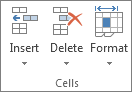
On the Home tab, in the Cells group, click Format.
-
Under Cell Size, do one of the following:
-
To fit all text in the cell, click AutoFit Column Width.
-
To specify a larger column width, click Column Width, and then type the width that you want in the Column width box.
-
Note: As an alternative to increasing the width of a column, you can change the format of that column or even an individual cell. For example, you could change the date format so that a date is displayed as only the month and day («mm/dd» format), such as 12/31, or represent a number in a Scientific (exponential) format, such as 4E+08.
Wrap text in a cell
You can display multiple lines of text inside a cell by wrapping the text. Wrapping text in a cell does not affect other cells.
-
Click the cell in which you want to wrap the text.
-
On the Home tab, in the Alignment group, click Wrap Text.
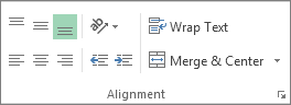
Note: If the text is a long word, the characters won’t wrap (the word won’t be split); instead, you can widen the column or decrease the font size to see all the text. If all the text is not visible after you wrap the text, you might have to adjust the height of the row. On the Home tab, in the Cells group, click Format, and then under Cell Size click AutoFit Row.
For more information on wrapping text, see the article Wrap text in a cell.
Change the format of a number
In Excel, the format of a cell is separate from the data that is stored in the cell. This display difference can have a significant effect when the data is numeric. For example, when a number that you enter is rounded, usually only the displayed number is rounded. Calculations use the actual number that is stored in the cell, not the formatted number that is displayed. Hence, calculations might appear inaccurate because of rounding in one or more cells.
After you type numbers in a cell, you can change the format in which they are displayed.
-
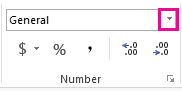
Click the cell that contains the numbers that you want to format.
-
On the Home tab, in the Number group, click the arrow next to the Number Format box, and then click the format that you want.
To select a number format from the list of available formats, click More Number Formats, and then click the format that you want to use in the Category list.
Format a number as text
For numbers that should not be calculated in Excel, such as phone numbers, you can format them as text by applying the Text format to empty cells before typing the numbers.
-
Select an empty cell.
-
On the Home tab, in the Number group, click the arrow next to the Number Format box, and then click Text.
-
Type the numbers that you want in the formatted cell.
Numbers that you entered before you applied the Text format to the cells must be entered again in the formatted cells. To quickly reenter numbers as text, select each cell, press F2, and then press Enter.
Need more help?
You can always ask an expert in the Excel Tech Community or get support in the Answers community.
Need more help?
Want more options?
Explore subscription benefits, browse training courses, learn how to secure your device, and more.
Communities help you ask and answer questions, give feedback, and hear from experts with rich knowledge.
To enter data in Excel, just select a cell and begin typing. You’ll see the text appear both in the cell and in the formula bar above. To tell Excel to accept the data you’ve typed, press enter. The information will be entered immediately, and the cursor will move down one cell.
Contents
- 1 How do I enter data into an Excel spreadsheet?
- 2 What are the two ways of entering data in Excel?
- 3 Can’t enter data Excel cell?
- 4 How do I insert data from a text file into Excel?
- 5 How can I enter data entry?
- 6 What are the three different ways of entering data in Excel?
- 7 How do you press enter in Excel and stay in the same cell?
- 8 How do I import data into Excel 2019?
- 9 How do you transpose data in Excel?
- 10 What is a CSV file in Excel?
- 11 What is data entry form in Excel?
- 12 What is data entry with example?
- 13 How many ways can you enter data in a cell?
- 14 Which cell is used to enter the data?
- 15 What is Ctrl enter in Excel?
- 16 When you type data in a cell and press Enter?
- 17 Can you flip data in Excel?
- 18 How do I paste data horizontally in Excel?
- 19 How do I open a .CSV file?
- 20 Is CSV and Excel same?
How do I enter data into an Excel spreadsheet?
On the worksheet, click a cell. Type the numbers or text that you want to enter, and then press ENTER or TAB. To enter data on a new line within a cell, enter a line break by pressing ALT+ENTER.
What are the two ways of entering data in Excel?
Text and number are two ways of entering data in Excel.
Can’t enter data Excel cell?
A cell won’t let me enter data
- The worksheet may have been protected.
- Cells may have been merged.
- Validation rules may be preventing the cell from being edited.
- The text may be invisible.
How do I insert data from a text file into Excel?
You can import data from a text file into an existing worksheet.
- Click the cell where you want to put the data from the text file.
- On the Data tab, in the Get External Data group, click From Text.
- In the Import Data dialog box, locate and double-click the text file that you want to import, and click Import.
How can I enter data entry?
Creating a New Entry
- Select any cell in the Excel Table.
- Click on the Form icon in the Quick Access Toolbar.
- Enter the data in the form fields.
- Hit the Enter key (or click the New button) to enter the record in the table and get a blank form for next record.
What are the three different ways of entering data in Excel?
You enter three types of data in cells: labels, values, and formulas. Labels (text) are descriptive pieces of information, such as names, months, or other identifying statistics, and they usually include alphabetic characters. Values (numbers) are generally raw numbers or dates.
How do you press enter in Excel and stay in the same cell?
To start a new line of text or add spacing between lines or paragraphs of text in a worksheet cell, press Alt+Enter to insert a line break. Double-click the cell in which you want to insert a line break (or select the cell and then press F2).
How do I import data into Excel 2019?
Import Data
- Click the Data tab on the Ribbon..
- Click the Get Data button. Some data sources may require special security access, and the connection process can often be very complex.
- Select From File.
- Select From Text/CSV.
- Select the file you want to import.
- Click Import.
- Verify the preview looks correct.
- Click Load.
How do you transpose data in Excel?
To transpose data, execute the following steps.
- Select the range A1:C1.
- Right click, and then click Copy.
- Select cell E2.
- Right click, and then click Paste Special.
- Check Transpose.
- Click OK.
What is a CSV file in Excel?
A CSV (comma-separated values) file is a simple text file in which information is separated by commas. CSV files are most commonly encountered in spreadsheets and databases. You can use a CSV file to move data between programs that aren’t ordinarily able to exchange data.
What is data entry form in Excel?
What Are Excel Forms? Excel offers the ability to make data entry easier by using a form, which is a dialog box with the fields for one record. The form allows data entry, a search function for existing entries, and the ability to edit or delete the data.
What is data entry with example?
Some examples of data entry job duties include transcribing, updating customer information, and entering accounting records.
How many ways can you enter data in a cell?
Following are some ways of entering data in the excel cells:
- Type directly into the cell.
- One can also use formula bar to enter data into the cell.
- Excel can speed up your data entry work through autocomplete.
- Autofill is another option to enter data.
Which cell is used to enter the data?
To make a cell reference absolute, you must include a $ before the reference (ex: $C$4). The other type of reference is a Relative Reference.. Active Cell: The active cell is the cell in the spreadsheet that is currently selected for data entry.
What is Ctrl enter in Excel?
#2 – Ctrl+Enter to Fill All Selected Cells with the Same Data or Formula. When we are entering data or a formula in a cell, and have multiple cells selected, Ctrl+Enter will copy the data/formula to all of the selected cells.
When you type data in a cell and press Enter?
By default when typing data or a formula into a cell and pressing enter, the active cell cursor will move down one cell. You don’t have to be stuck with this if you don’t want it though. You can also have it go up, left, right or not move at all if you want.
Can you flip data in Excel?
Just select a range of cells you want to flip, go to the Ablebits Data tab > Transform group, and click Flip > Horizontal Flip.
How do I paste data horizontally in Excel?
Here’s how:
- Select the range of data you want to rearrange, including any row or column labels, and either select Copy.
- Select the first cell where you want to paste the data, and on the Home tab, click the arrow next to Paste, and then click Transpose.
How do I open a .CSV file?
You can also open CSV files in spreadsheet programs, which make them easier to read. For example, if you have Microsoft Excel installed on your computer, you can just double-click a . csv file to open it in Excel by default. If it doesn’t open in Excel, you can right-click the CSV file and select Open With > Excel.
Is CSV and Excel same?
CSV and Excel or xls are two different types of file extensions which both contain data in them, the difference between the both is that in CSV or comma-separated values the data is in text format separated by commas while in excel or Xls data is in tabular format or we say in rows and columns and in CSV file extension
Once you know how to enter data into an Excel worksheet you will be setting up tables of data in no time.
When you haven’t been shown how to enter data it can be a little tricky, so follow the steps below to learn the tips and hacks to entering your data easily into your worksheet.
Entering data into an Excel worksheet
You can enter either values (numbers and dates) or labels (text) into any cell within the worksheet.
1. Move the cell pointer to the required cell and then type the data. While you type the data you will notice that it appears both in the worksheet (in the example below, the text appears in cell A1) and in the Formula Bar.
2. Press ENTER to enter the information into the cell. Your cell pointer will move down to the cell below.
Tip: If you press the ESC key instead of ENTER the data will not be entered into the cell.
Deleting and replacing data
- To delete data select the cell containing the data and then press DELETE.
- To replace data just type directly over the top of the existing cell contents. The new data will replace the old.
Using Undo and Redo
There will be times when you enter data only to realise you have made a bit of a mess of things.
Most times you want to back-back to where you were before the mistake was made. If this happens you can click the fabulous “Undo” button which will undo the last thing you did.
You can actually keep clicking it until you get back to a point where you feel in control again.
And if you go one step to far back, you can click the Redo button to go forward a step again. These buttons are fabulous and you use them a lot.
Overlapping data
If you enter data that will not fit the column width it will overlap into the next column. In the example below the text ‘Travel Expenses’ is entered into cell A1, however it looks as though the text is included in cells B1. With cell A1 selected we can see in the Formula bar that both words are indeed in A1.
If you are not using the column into which the text is overlapping you may leave the text as it is. However, as soon as you place text into a cell that has been overlapped it will look as if your text has been lost. In the example below, the text ‘Amount ex GST’ has been entered into cell C3. However the content of cell D3 is hiding part of the content is C3.
By selecting C3 the entire cell’s content can be seen in the Formula Bar. In order to view the entire contents of cell C3 the width of column C needs to be adjusted.
Working with columns
The standard column width for Excel is 8.43 character spaces. You can change the column width by dragging with your mouse on the column headers, or by double clicking between two column headers.
Tip: If multiple columns require the same width, select the columns and widen one of them with the mouse. The rest will be adjusted to the same width.
Adjusting the column width
To use your mouse to adjust the column width:
1. Move your mouse pointer over the column’s right edge in the column header area. Your mouse pointer should change to a double-headed arrow.
2. Click and drag to the right to expand, or to the left to shrink the column width to the size you require.
You will now be able to see your entire text. Continue dragging until all columns are the width you require.
Tips:
To quickly adjust the column width to fit the widest entry, move your mouse pointer over the lines between the column headers. When the pointer becomes a double-headed arrow double-click.
Use the same method for adjusting the height of any row. Just move the mouse pointer over the line separating the rows. When the pointer becomes a double-headed arrow, drag or double-click to adjust the row height, or double-click to set the height to fit the tallest entry.
By the way, row heights will automatically alter if the font size of data is altered.
Extra info: to set a column width to a precise measurement on the Home tab in the Cells group select Format and then select Column Width. Type the desired width in the Column Width box and then click OK to accept the new column width.
What do hash signs mean in Excel?
If you ever see a cell containing ######## (hash signs) it means the column isn’t wide enough to display the content. Just extend the width and the content will become visible.
Making changes to the data
Once you have entered data into your worksheet, you can edit the data in a number of ways.
- Select the cell and then click in the Formula bar. A flashing insertion point will be placed into the bar. Use the arrow keys on the keyboard to move the insertion point. Make the changes you require and then press ENTER.
- You may also type directly over the data in the cell with new data and then press ENTER. The new data will replace the old.
- Double clicking a cell or pressing F2 allows you to edit the contents of the cell directly on the worksheet. Make the changes and then press ENTER to update the cell.
AutoComplete
AutoComplete is the ability for Excel to automatically complete an entry for you.
For example, if you have typed text in the cells above as soon as you start typing a letter or two in a cell below, Excel will check the list above for a matching entry and complete the entry for you.
This can be very useful when you need to make the same entry several times.
To accept the entry press ENTER. To reject the displayed entry and type something different either ignore the entry and type right over it or press DELETE.
Was this blog helpful? Let us know in the Comments below.
Instructions
Entering data into an Excel worksheet
- Move the cell pointer to the required cell and then type the data.
- Press ENTER to enter the information into the cell. Your cell pointer will move down to the cell below.
Deleting and replacing data
To Delete: Select the cell containing the data and then press DELETE.
To replace data: Type directly over the top of the existing cell contents. The new data will replace the old.
Using Undo and Redo
If you make a mistake, you can use the Undo button on the top right of the Excel spreadsheet to undo the last thing you did. You can keep clicking it to go back multiple steps.
If you Undo something you didn’t want undone, you can use the Redo button to the right of the Undo button to go forward a step again.
Overlapping data
If you enter data that will not fit the column width it will overlap into the next column. Adjust the width of the columns in order to view the entire contents.
Working with columns
Adjusting the column width
- Move your mouse pointer over the column’s right edge in the column header area. Your mouse pointer should change to a double-headed arrow.
- Click and drag to the right to expand, or to the left to shrink the column width to the size you require.
- You will now be able to see your entire text. Continue dragging until all columns are the width you require.
Making changes to the data
- Select the cell and then click in the Formula bar. A flashing insertion point will be placed into the bar. Use the arrow keys on the keyboard to move the insertion point. Make the changes you require and then press ENTER.
- You may also type directly over the data in the cell with new data and then press ENTER. The new data will replace the old.
- Double clicking a cell or pressing F2 allows you to edit the contents of the cell directly on the worksheet. Make the changes and then press ENTER to update the cell.
AutoComplete
Sometimes when you are typing in a cell, Excel will automatically complete the entry for you. To accept the entry press ENTER. To reject the displayed entry and type something different either ignore the entry and type right over it or press DELETE.
Notes
Note: While you type the data you will notice that it appears both in the worksheet cell and in the Formula Bar.
Tip: If you press the ESC key instead of ENTER when typing data into a cell the data will not be entered into the cell.
Tips: To quickly adjust the column width to fit the widest entry, move your mouse pointer over the lines between the column headers. When the pointer becomes a double-headed arrow double-click.
Extra info: to set a column width to a precise measurement on the Home tab in the Cells group select Format and then select Column Width. Type the desired width in the Column Width box and then click OK to accept the new column width.
Note: If you ever see a cell containing ######## (hash signs) it means the column isn’t wide enough to display the content. Just extend the width and the content will become visible.
Some users are experiencing an issue with Excel. According to them, they are not able to type in any of the cells in an Excel spreadsheet. Also, there are no macros enabled and the Excel sheet or cells are not protected. If you are unable to type in Excel, you can refer to the solutions listed in this article to get rid of the problem.

The troubleshooting guidelines to deal with this problem are explained below. But before you proceed, close all the Excel files and open Excel again. Now, check if you can type something in your Excel spreadsheet. If Excel won’t let you type this time too, restart your computer and check the status of the issue.
Some users were able to fix the problem by doing the following trick:
- Open a new blank Excel spreadsheet.
- Type something in the new spreadsheet.
- Now, type in the original (problematic) spreadsheet.
You can also try the above trick and check if it helps. If the issue persists, try the following fixes.
- Check the Editing options setting
- Troubleshoot Excel in Safe mode
- Move files from the C directory to another location
- Uninstall the recently installed software
- Disable the Hardware Graphic Acceleration in Excel
- Change the Trust Center settings
- Repair Office
- Uninstall and reinstall Office
Below, we have explained all these fixes in detail.
1] Check the Editing options setting
If the “Allow editing directly in cells” option is disabled in Excel Editing settings, you may experience this type of problem. To check this, go through the following instructions:

- Open Excel file.
- Go to “File > Options.”
- Select Advanced from the left pane.
- The “Allow editing directly in cells” checkbox should be enabled. If not, enable it and click OK.
2] Troubleshoot Excel in Safe mode
The problem might be occurring due to some Excel Add-ins. You can check this by troubleshooting Excel in Safe mode. Some of the Add-ins remain disabled in the Safe mode. Hence, launching an Office application in Safe mode makes it easier to identify the problematic Add-in.
The process to troubleshoot Excel in Safe mode is as follows:
- Save your spreadsheet and close Excel.
- Open the Run command box (Win + R keys) and type
excel /safe. After that click OK. This will launch Excel in the Safe mode. - After launching Excel in Safe mode, type something in cells. If you are able to type in the Safe mode, one of the Add-ins disabled in the Safe mode by default is the culprit. If you are unable to type in the Safe mode, one of the Add-ins enabled in the Safe mode is the culprit. Let’s see these two cases in detail.
Case 1: You are able to type in the Safe mode
- In the Safe mode, go to “File > Options.”
- Select Add-Ins from the left side.
- Now, select COM Add-ins in the drop-down and click Go. After that, you will see all the Add-ins that are enabled in the Safe mode. Because you are able to type in the Safe mode, none of these Add-ins is causing the problem. Take a note of the Add-ins that are enabled in the Safe mode.
- Close Excel in the Safe mode and open Excel in the normal mode.
- Go to “File > Options > Add-Ins.” Select COM Add-ins in the drop-down and click Go.
- Disable any of the enabled Add-ins and click OK. Do not disable the Add-ins that were enabled in the Safe mode.
- After disabling an Add-in, restart Excel in normal mode and check if you are able to type. If yes, the Add-in that you have disabled recently was causing the problem. If not, repeat steps 5 to 7 to identify the problematic Add-in. Once you find it, consider removing it.
Case 2: You are unable to type in the Safe mode
- In the Safe mode, go to “File > Options > Add-Ins.” Select COM Add-ins in the drop-down and click Go.
- Disable any of the Add-ins and click OK.
- Now, type something. If you are able to type, the Add-in that you have disabled recently was causing the problem. Remove that Add-in.
- If you are unable to type, disable another Add-in in the Safe mode and then check again.
3] Move files from the C directory to another location
Move the Excel files from the C directory to another location and check if the problem disappears or not. Follow the instructions listed below.
- First, close Excel.
- Open the Run command box and type
%appdata%MicrosoftExcel. Click OK. This will open the Excel folder in your C drive. It is a temporary location for unsaved files. Excel saves your files here temporarily so that they could be recovered in case Excel crashes or your system shuts down unexpectedly. - Move all the files to another location and make the Excel folder empty. After that, open Excel and check if the problem disappears. If this does not fix the issue, you can place all the files back in the Excel folder.
4] Uninstall the recently installed software
If the problem started occurring after installing an app or software, that app or software may be the cause of the problem. To check this, uninstall the recently installed app or software and then check if you can type in Excel. Some users have found the following third-party applications the cause of the problem:
- Tuneup Utilities
- Abby Finereader
If you have installed any of the above software, uninstall them and check if the problem disappears.
Read: Excel freezing, crashing or not responding.
5] Disable the Hardware Graphics Acceleration in Excel
If the Hardware Graphics Acceleration is enabled in Excel, that may be causing the problem. You can check this by disabling the Hardware Graphics Acceleration. The steps for the same are as follows:

- Open Excel.
- Go to “File > Options.”
- Select the Advanced category on the left side.
- Scroll down and locate the Display section.
- Uncheck the Disable hardware graphics acceleration checkbox.
- Click OK.
6] Change the Trust Center settings
Change the Trust Center settings and see if this fixes the issue. The following steps will help you with that.

- Open Excel.
- Go to “File > Options.” This will open the Excel Options window.
- Select the Trust Center category from the left side and click on the Trust Center Settings button.
- Now, select Protected View from the left side and uncheck all the options.
- Select File Block Settings from the left pane and uncheck all the options.
- Click OK to save the settings.
7] Repair Office
If despite trying all the above fixes, the problem still persists, some of the Office files might be corrupted. In such a case, an Online Office Repair may fix the problem.
8] Uninstall and reinstall Office
If the online repair fails to fix the problem, uninstall Microsoft Office and install it again. You can uninstall Microsoft Office from the Control Panel or from Windows 11/10 Settings.
Read: How to fix high CPU usage by Excel.
Why is my Excel not allowing me to type?
There are several reasons why Excel is not allowing you to type, like incorrect Editing settings, conflicting apps or software, etc. Apart from that, problematic Add-ins also cause several issues in Microsoft Office applications. You can identify which Add-in is causing the problem by troubleshooting Excel in the Safe mode.
Sometimes, the Hardware Graphics Acceleration or Protected view causes problems in Excel. You can change the Trust Center settings and see if this fixes the problem.
If some Office files get corrupted due to some reason, you may experience different errors in different Office applications. Such a type of problem can be fixed by running an online repair.
How do I unlock my keyboard in Excel?
If you turn on Scroll Lock in Excel, you can move the entire sheet by using the arrow keys. To unlock your keyboard in Excel, turn off the Scroll Lock.
Hope this helps.
Read next: Fix Errors were detected while saving the Excel file.
Transcript
In this lesson, we’ll look at the most basic way to enter data in an Excel worksheet—by typing. In future lessons, we’ll look at a number of shortcuts for entering data faster.
To enter data in Excel, just select a cell and begin typing. You’ll see the text appear both in the cell and in the formula bar above.
To tell Excel to accept the data you’ve typed, press enter. The information will be entered immediately, and the cursor will move down one cell.
You can also press the tab key instead of the enter key. If you press tab, the cursor will move one cell to the right once the information has been entered.
When Excel sees that you are typing into a list, pressing enter at the end of the row will move the cursor down one row and back to the first column.
At any time while you are typing you can press the escape key to cancel. This brings Excel back to the state it was in before you started typing.
When you want to delete information that has already been entered, just select the cells, and press the delete key.

Author![]()
Dave Bruns
Hi — I’m Dave Bruns, and I run Exceljet with my wife, Lisa. Our goal is to help you work faster in Excel. We create short videos, and clear examples of formulas, functions, pivot tables, conditional formatting, and charts.
Entering data into Excel is exactly the same across all Excel versions and can be done in a number of different ways.
The first way you can enter data into Excel is using the formula bar. First you click on a cell, A1 for example and then you click on the formula bar so that the cursor appears within it.
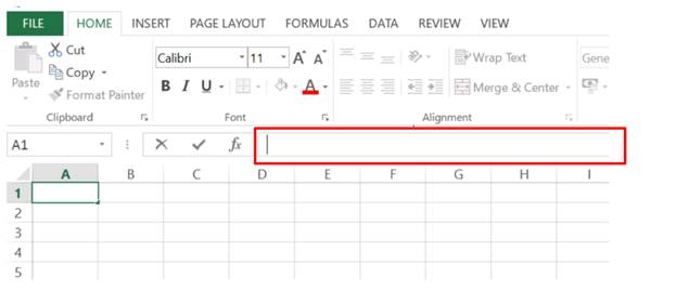
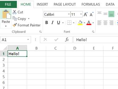
You can now type using the keyboard to enter data into cell A1. I typed Hello! into the formula bar and it also appears in the cell I had selected (A1):
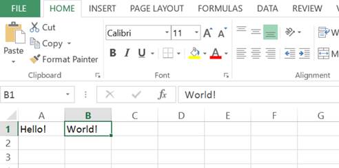
This also works by typing directly into the selected cell (without clicking on the formula bar). So if I select cell B2 and type World! it appears in the selected cell and the formula bar in exactly the same way:
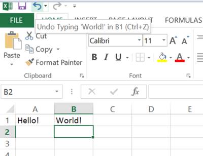
If you dont like what youve typed into a particular cell you can undo the action much like in Word and other Office programs. This is done by clicking the Undo button. This is the backwards pointing arrow in the top left corner of Excel. By hovering the mouse over this button the undo action that will be performed is shown. So as the last thing I did was type World! into cell B1, clicking the undo button will remove world from cell B1.
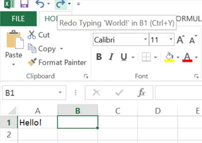
In addition to the Undo button there is also the Redo button. This is the forward pointing arrow and this re-does what you have just undone with the Undo button. So as I just used Undo to remove World! from cell B2, the Redo button will re-enter World! into cell B2.
Alternatively I could have used the keyboard shortcut Ctrl + Z to undo and Ctrl + Y to redo. These work the exact same way as clicking the buttons.
The Ctrl + Y shortcut for redo has some additional functionality. It can be used to repeat actions such as copying formats to other cells. I will go through how this feature works in more detail in the next tutorial as it saves time when making changes to individual or groups of cells.
![]()
Excel VBA Course — From Beginner to Expert
200+ Video Lessons
50+ Hours of Instruction
200+ Excel Guides
Become a master of VBA and Macros in Excel and learn how to automate all of your tasks in Excel with this online course. (No VBA experience required.)
View Course
Similar Content on TeachExcel
Use a Form to Enter Data into a Table in Excel
Tutorial:
You can enter data into a table in Excel using a form; here I’ll show you how to do that….
Put Data into a UserForm
Tutorial: How to take data from Excel and put it into a UserForm. This is useful when you use a form…
Put Data into a Worksheet using a Macro in Excel
Tutorial: How to input data into cells in a worksheet from a macro.
Once you have data in your macro…
VBA Macro to Import Web Data into Excel
Tutorial:
It’s time to learn how to use VBA and Macros to import data from a web page into Excel!
T…
How to Use Dates in Excel
Tutorial:
Introduction Guide to using Dates in Excel — this tutorial will show you how to input and…
Simple Alternatives to UserForms
Tutorial: This tutorial covers a few simple ways to show pop-up windows to users that allows you to …
Subscribe for Weekly Tutorials
BONUS: subscribe now to download our Top Tutorials Ebook!
![]()
Excel VBA Course — From Beginner to Expert
200+ Video Lessons
50+ Hours of Video
200+ Excel Guides
Become a master of VBA and Macros in Excel and learn how to automate all of your tasks in Excel with this online course. (No VBA experience required.)
View Course
Excel is an amazing tool with fascinating capabilities to analyze data (be it using functions, charts or dashboards). The ease with which data can be entered and stored in Excel makes it a compelling choice.
In this blog post, I have listed 10 useful Excel Data Entry tips that will make you more efficient and save a lot of time.
#1 Use Excel Data Entry Form
Excel Data Entry form enables you to add records to an existing data set. It gives a pop-up form that can be filled by the user. It is especially convenient when the data set has many columns and would require you to scroll right and left again and again as you key in data points.
Data Form feature is not already available in Excel ribbon. We first need to make it available by adding it to the Quick Access toolbar.
Adding Excel Data Entry Form to Quick Access Toolbar
- Go to Quick Access Toolbar, right-click and select Customize quick Access Toolbar.

- In the Excel Options Dialogue box, Select All Commands and Go to Form. Select Form and press Add. This will add the Data Forms Icon to the Quick Access Toolbar.


Using Excel Data Entry Form
- Select any cell in the data range and click on the Data Form icon from the Quick Access Toolbar.
- In the Pop-up Data form, all the column titles are listed vertically. Fill the data in the adjacent text box for each heading.
- Once you have entered the data, press Enter.
- Click on New to add a new record.
Using Excel Data Entry form, you can also navigate through the existing data (row by row), or find data by specifying the criteria (try this by clicking on the criteria button).
#2 Quickly Enter Numbers with Fixed Decimal Numbers
If you are in a situation where you have to manually enter data in excel that also has a decimal part to it, this trick could be mighty useful. For example, suppose you have to enter marks for students in percentage with up to 2 decimal points. You can enable a feature where you just type the numbers without bothering about hitting the dot key every time. To enable this:
- Go To File –> Options.
- In the Excel Options Dialogue box, select Advanced.
- In Advanced Options, check the option “Automatically Insert a decimal point”.
- Specify the number of decimals you want (for example 2 in this case).
Now, whenever you enter any number, excel automatically places last 2 digits after the decimal. So 1 becomes .01, 10 becomes 0.1, 100 becomes 1, 2467 becomes 24.67 and so on..

Once you are done with data entry, simply switch it off by un-checking the same option.
#3 Automatically Add Ordinal to Numbers
Yes, you can use a combination of excel functions (such as VALUE, RIGHT, IF, OR) to add ordinals (‘st’ in 1st, ‘nd’ in 2nd, and so on..).
Here is the formula:
=A1&IF(OR(VALUE(RIGHT(A1,2))={11,12,13}),"th",IF(OR(VALUE(RIGHT(A1))={1,2,3}),CHOOSE(RIGHT(A1),"st","nd","rd"),"th"))
#4 Fill Down Using Control + D
This is a nifty Excel Data Entry trick. If you have to copy the above cell, just press Control + D.
It copies the content as well as the formatting. If there is a formula in the above cell, the formula is copied (with adjusted references).
This works for more than one cell as well. So if you want to copy the entire row above, select the current row and press Control + D.
If you select more than one cell/cells, than the cell above selection is copied to all the cells.
See Also: 200+ Excel Keyboard Shortcuts.
#5 Quickly Enter Date/Time in Excel Cells
Do not remember the current date? Don’t worry, just press Control + ; (semicolon Key) and it will enter the current date in the cell.
Similarly, you can enter current time by using the shortcut Control + Shift + : (colon key)
Remember, these are absolute values, and won’t change if the date or time changes. If you want to have a dynamic date and time value that changes whenever you open the workbook or when there is a re-calculation, use TODAY and NOW functions.
Also See: How to Automatically Insert Date and Time Stamp in Excel.
#6 Control + Enter to Fill Entire Selection with Content in Active Cell
When you select multiple cells in Excel, one of the cells with light shade (as compared with the remaining selected cells) is the active cell. If you enter something in the active cell when the selection is made and press Control + Enter, the value is inserted into all the selected cells.
This holds true for formulas as well. If you enter a formula in the active cell and press Control + Enter, all the cells will get that formula (with adjusted references).
#7 Alt + Down Arrow to Get a List of All Unique Values in that column
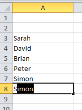
This one can save some time that you might otherwise waste in typing. Suppose you are entering data in a column with activity status (To be Done, Completed). Instead of typing the status, again and again, you just need to type it in a couple of cells, and then you can use the keyboard shortcut Alt + Down arrow. It gives you the list all the unique entries, and you can quickly select from the list.
![]()
If you want to select from pre-specified options, you can create a drop down list.
#8 Quickly Sift through Multiple Worksheet Tabs in a Workbook
This one saves tons of time. Simply use the keyboard shortcut Control + Page Up/Page Down to navigate through multiple worksheet tabs in a workbook.
See Also: 200+ Excel Keyboard Shortcuts.
#9 Enter Long Text by Using Abbreviations
If you have to enter long names or keywords again and again in your worksheet, this trick would come in handy.
For example, you may want that whenever you type ABC, Excel should automatically replace it with ABC Technology Corporation Limited.
Something as shown below:
This feature can be enabled using the autocorrect options. Read how to enable it.
#10 Enter Data in Non-Contiguous Ranges
Suppose you have a template as shown below, and you have to enter data in all the cells highlighted in red, in the order specified by the arrows.

Here is a quick way to do this:
- Select all the cells where you need to enter the data (press control and then select one by one).
- Start with the second cell in your sequence of data entry (start with D3). Select the first cell B3 (where data entry begins) at last.
- Once selected, go to Name Box (which is on the left of the formula bar).
- Type any name without spaces.
- That’s It!! Select the Named Range by clicking the Name Box drop-down. Now start entering your data and use Enter/Tab to jump to the next cell.
Read more about this trick.
These are my top ten excel data entry tips that can significantly improve your productivity and save time.
You May Also Like the Following Excel Tips:
- 10 Super Neat Ways to Clean Data in Excel Spreadsheets.
- 24 Daily Excel Issues and their Quick Fixes.
- How to Track Changes in Excel.
- How to Recover Unsaved Excel Files.
- How to Enable Conditional Data Entry in Excel.
- Suffering from Slow Excel Spreadsheets? 10 tips to SPEED-UP your Excel.
- Get more out of Find and Replace in Excel (4 Amazing Tips).
- How to Use Excel Freeze Panes in Excel.
- 100+ Excel Interview Questions
- Fill Down Blank Cells Until the Next Value in Excel
There is more than one way to enter data into an Excel worksheet. Sometimes we stick to typing directly into cells, but there are different ways to enter data which can speed up your data entry work.
- Type directly into a cell and add your data. You know a cell is active as it is highlighted with a darker border.

A2 is the active cell – it has a darker border so it stands out from the other cells - Use the formula bar. This is located under the ribbon. Type your data directly into the formula bar and press enter. You can navigate around the worksheet by typing the cell number directly into the Name box (located above the Column headings A – Z).

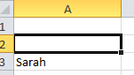
The Name Box shows that the active cell is A3. - Make the most of autocomplete. Excel will try to help you speed up your data entry by guessing what you are typing based on what’s in your worksheet. If the autocorrect option is right for you, just press enter.

Autocomplete is guessing that I am typing Simon, and I’ve just typed “Si”, I can press enter and the full name is entered for me. - Copy and paste – you may have cells that you can copy and paste data within the same worksheet – it can save you time formatting a sheet, or you can copy data to another worksheet within the workbook.
- Let Autofill do the work. Autofill options can complete series of data, whether it is text or numbers. This saves lots of data entry when setting up worksheets, or entering data.

Computer Excel training can give you extra skills so you can speed up entering the data, so you can concentrate on using the information you’ve gathered. https://www.stl-training.co.uk/excel-2007-introduction.php
Data entry can sometimes be a big part of using Excel.
With near endless cells, it can be hard for the person inputting data to know where to put what data.
A data entry form can solve this problem and help guide the user to input the correct data in the correct place.
Excel has had VBA user forms for a long time, but they are complicated to set up and not very flexible to change.
In this blog post, we’re going to explore 5 easy ways to create a data entry form for Excel.
Video Tutorial
Excel Tables
We’ve had Excel tables since Excel 2007.
They’re perfect data containers and can be used as a simple data entry form.
Creating a table is easy.
- Select the range of data including the column headings.
- Go to the Insert tab in the ribbon.
- Press the Table button in the Tables section.
We can also use a keyboard shortcut to create a table. The Ctrl + T keyboard shortcut will do the same thing.
Make sure the Create Table dialog box has the My table has headers option checked and press the OK button.
We now have our data inside an Excel table and we can use this to enter new data.
To add new data into our table we can start typing a new entry into the cells directly below the table and the table will absorb the new data.
We can use the Tab key instead of Enter while entering our data. This will cause the active cell cursor to move to the right instead of down so we can add the next value into our record.
When the active cell cursor is in the last cell of the table (lower right cell), pressing the Tab key will create a new empty row in the table ready for the next entry.
This is a perfect and simple data entry form.
Data Entry Form
Excel actually has a hidden data entry form and we can access it by adding the command to the Quick Access Toolbar.
Add the form command to the Quick Access Toolbar.
- Right click anywhere on the quick quick access toolbar.
- Select Customize Quick Access Toolbar from the menu options.
This will open up the Excel option menu on the Quick Access Toolbar tab.
- Select Commands Not in the Ribbon.
- Select Form from the list of available commands. Press F to jump to the commands starting with F.
- Press the Add button to add the command into the quick access toolbar.
- Press the OK button.
We can then open up data entry form for any set of data.
- Select a cell inside the data which we want to create a data entry form with.
- Click on the Form icon in the quick access toolbar area.
This will open up a customized data entry form based on the fields in our data.
Microsoft Forms
If we need a simple data entry form, why not use Microsoft Forms?
This form option will require our Excel workbook to be saved into SharePoint or OneDrive.
The form will be in a browser and not in Excel, but we can link the form to an Excel workbook so that all the data goes into our Excel table.
This is a great option if multiple people or people outside our organization need to input data into the Excel workbook.
We need to create a Form for Excel in either SharePoint or OneDrive. The process is the same for both SharePoint or OneDrive.
- Go to a SharePoint document library or a OneDrive folder where the Excel workbook is going to be saved.
- Click on New and then choose Forms for Excel.
This will prompt us to name the Excel workbook and open up a new browser tab where we can build our form by adding different types of questions.
We first need to create the Form and this will create the table in our Excel workbook where the data will get populated.
Then we can share the form with anyone we want to input data into Excel.
When a user enters data into the form and presses the submit button, that data will automatically show up into our Excel workbook.
Power Apps
Power Apps is a flexible drag and drop formula based app building platform from Microsoft.
We can certainly use it to create a data entry from for our Excel data.
In fact, if we have a table of data set up, Power Apps will create the app for us based on our data. It can’t be any easier than that.
Sign in to the powerapps.microsoft.com service ➜ go to the Create tab in the navigation pane ➜ select Excel Online.
We’ll then be prompted to sign in to our SharePoint or OneDrive account where our Excel file is saved to select the Excel workbook and table with our data.
This will generate us a fully functional three screen data entry app.
- We can search and view all the records in our Excel table in a scroll-able gallery.
- We can view an individual record in our data.
- We can edit an existing record or add new records.
This is all connected to our Excel table, so any changes or additions from the app will show up in Excel.
Power Automate
Power Automate is a cloud based tool for automating task between apps.
But we can use the button trigger to make an automation that captures user input and adds the data into an Excel table.
We’ll need to have our Excel workbook saved in OneDrive or SharePoint and have a table already setup with the fields we want to populate.
To create our Power Automate data entry form.
- Go to flow.microsoft.com and sign in.
- Go to the Create tab.
- Create an Instant flow.
- Give the flow a name.
- Choose the Manually trigger a flow option as the trigger.
- Press the Create button.
This will open up the Power Automate builder and we can build our automation.
- Click on the Manually trigger a flow block to expand the trigger’s options. This is where we’ll find the ability to add input fields.
- Click on the Add an input button. This will give us options to add a few different types of input fields including Text, Yes/No, Files, Email, Number and Dates.
- Rename the field to something descriptive. This will help the user know what type of data to input when they run this automation.
- Click on the three ellipses to the right of each field to change the input options. We’ll be able to Add a drop-down list of option, Add a multi-select list of options, Make the field optional or Delete the field from this menu.
- After we have added all our input fields, we can now add a New step to the automation.
Search for the Excel connector and add the Add a row into a table action. If you’re on an Office 365 business account, use the Excel Online (Business) connectors, otherwise use the Excel Online (OneDrive) connectors.
Now we can set up our Excel Add a row into a table step.
- Navigate to the Excel file and table where we are going to be adding data.
- After selecting the table, the fields in that table will appear listed and we can add the appropriate dynamic content from the Manually trigger a flow trigger step.
Now we can run our Flow from the Power Automate service.
- Go to My flows in the left navigation pane.
- Go to the My flows tab.
- Find the flow in the list of available flows and click on the Run button.
- A side pane will pop up with our inputs and we can enter our data.
- Click Run flow.
We can also run this from our mobile device with the Power Automate apps.
- Go to the Buttons section in the app.
- Press on the flow to run.
- Enter the data inputs in the form.
- Press on the DONE button in the top right.
Whichever way we run the flow, a few seconds later the data will appear in our Excel table.
Conclusions
Whether we require a simple form or something more complex and customize-able, there is a solution for our data entry needs.
We can quickly create something inside our workbook or use an external solution that connects to and loads data into Excel.
We can even create forms that people outside our organization can use to populate our spreadsheets.
Let me know in the comments what is your favourite data entry form option.
About the Author
John is a Microsoft MVP and qualified actuary with over 15 years of experience. He has worked in a variety of industries, including insurance, ad tech, and most recently Power Platform consulting. He is a keen problem solver and has a passion for using technology to make businesses more efficient.