
Use calculated columns in an Excel table
Excel for Microsoft 365 Excel for Microsoft 365 for Mac Excel 2021 Excel 2021 for Mac Excel 2019 Excel 2019 for Mac Excel 2016 Excel 2016 for Mac Excel 2013 Excel 2010 Excel 2007 Excel for Mac 2011 More…Less
Calculated columns in Excel tables are a fantastic tool for entering formulas efficiently. They allow you to enter a single formula in one cell, and then that formula will automatically expand to the rest of the column by itself. There’s no need to use the Fill or Copy commands. This can be incredibly time saving, especially if you have a lot of rows. And the same thing happens when you change a formula; the change will also expand to the rest of the calculated column.
Note: The screen shots in this article were taken in Excel 2016. If you have a different version your view might be slightly different, but unless otherwise noted, the functionality is the same.
Create a calculated column
-
Create a table. If you’re not familiar with Excel tables, you can learn more at: Overview of Excel tables.
-
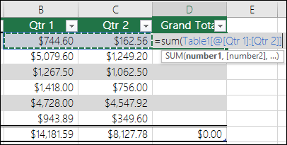
Insert a new column into the table. You can do this by typing in the column immediately to the right of the table, and Excel will automatically extend the table for you. In this example, we created a new column by typing «Grand Total» into cell D1.

Tips:
-
You can also add a table column from the Home tab. Just click on the arrow for Insert > Insert Table Columns to the Left.
-
-
-
Type the formula that you want to use, and press Enter.
In this case we entered =sum(, then selected the Qtr 1 and Qtr 2 columns. As a result, Excel built the formula: =SUM(Table1[@[Qtr 1]:[Qtr 2]]). This is called a structured reference formula, which is unique to Excel tables. The structured reference format is what allows the table to use the same formula for each row. A regular Excel formula for this would be =SUM(B2:C2), which you would then need to copy or fill down to the rest of the cells in your column
To learn more about structured references, see: Using structured references with Excel tables.
-
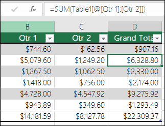
When you press Enter, the formula is automatically filled into all cells of the column — above as well as below the cell where you entered the formula. The formula is the same for each row, but since it’s a structured reference, Excel knows internally which row is which.


Notes:
-
Copying or filling a formula into all cells of a blank table column also creates a calculated column.
-
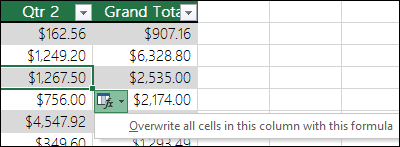
If you type or move a formula in a table column that already contains data, a calculated column is not automatically created. However, the AutoCorrect Options button is displayed to provide you with the option to overwrite the data so that a calculated column can be created.
-
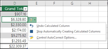
If you input a new formula that is different from existing formulas in a calculated column, the column will automatically update with the new formula. You can choose to undo the update, and only keep the single new formula from the AutoCorrect Options button. This is generally not recommended though, because it can prevent your column from automatically updating in the future, since it won’t know which formula to extend when new rows are added.
-
If you typed or copied a formula into a cell of a blank column and don’t want to keep the new calculated column, click Undo
twice. You can also press Ctrl + Z twice
 twice. You can also press Ctrl + Z twice
A calculated column can include a cell that has a different formula from the rest. This creates an exception that will be clearly marked in the table. This way, inadvertent inconsistencies can easily be detected and resolved.
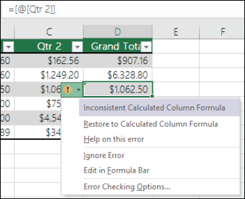
Note: Calculated column exceptions are created when you do any of the following:
-
Type data other than a formula in a calculated column cell.
-
Type a formula in a calculated column cell, and then click Undo
on the Quick Access Toolbar. -
Type a new formula in a calculated column that already contains one or more exceptions.
-
Copy data into the calculated column that does not match the calculated column formula.
Note: If the copied data contains a formula, this formula will overwrite the data in the calculated column.
-
Delete a formula from one or more cells in the calculated column.
Note: This exception is not marked.
-
Move or delete a cell on another worksheet area that is referenced by one of the rows in a calculated column.
Error notification will only appear if you have the background error checking option enabled. If you don’t see the error, then go to File > Options > Formulas > make sure the Enable background error checking box is checked.
-
If you’re using Excel 2007, click the Office button
, then Excel Options > Formulas. -
If you’re using a Mac, go to Excel on the menu bar, and then click Preferences > Formulas & Lists > Error Checking.
 , then Excel Options > Formulas.
The option to automatically fill formulas to create calculated columns in an Excel table is on by default. If you don’t want Excel to create calculated columns when you enter formulas in table columns, you can turn the option to fill formulas off. If you don’t want to turn the option off, but don’t always want to create calculated columns as you work in a table, you can stop calculated columns from being created automatically.
-
Turn calculated columns on or off
-
On the File tab, click Options.
If you’re using Excel 2007, click the Office button
, then Excel Options. -
Click Proofing.
-
Under AutoCorrect options, click AutoCorrect Options.
-
Click the AutoFormat As You Type tab.
-
Under Automatically as you work, select or clear the Fill formulas in tables to create calculated columns check box to turn this option on or off.
Tip: You can also click the AutoCorrect Options button that is displayed in the table column after you enter a formula. Click Control AutoCorrect Options, and then clear the Fill formulas in tables to create calculated columns check box to turn this option off.
If you’re using a Mac, goto Excel on the main menu, then Preferences > Formulas and Lists > Tables & Filters > Automatically fill formulas.
-
-
Stop creating calculated columns automatically
After entering the first formula in a table column, click the AutoCorrect Options button that is displayed, and then click Stop Automatically Creating Calculated Columns.

You can also create custom calculated fields with PivotTables, where you create one formula and Excel then applies it to an entire column. Learn more about Calculating values in a PivotTable.
Need more help?
You can always ask an expert in the Excel Tech Community or get support in the Answers community.
See Also
Overview of Excel tables
Format an Excel table
Resize a table by adding or removing rows and columns
Total the data in an Excel table
Need more help?
Want more options?
Explore subscription benefits, browse training courses, learn how to secure your device, and more.
Communities help you ask and answer questions, give feedback, and hear from experts with rich knowledge.
Formulas are the life and blood of Excel spreadsheets. And in most cases, you don’t need the formula in just one cell or a couple of cells.
In most cases, you would need to apply the formula to an entire column (or a large range of cells in a column).
And Excel gives you multiple different ways to do this with a few clicks (or a keyboard shortcut).
Let’s have a look at these methods.
By Double-Clicking on the AutoFill Handle
One of the easiest ways to apply a formula to an entire column is by using this simple mouse double-click trick.
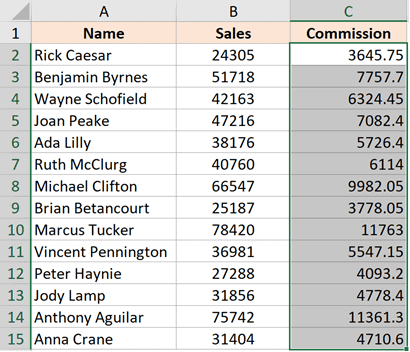
Suppose you have the dataset as shown below, where want to calculate the commission for each sales rep in Column C (where the commission would be 15% of the sale value in column B).
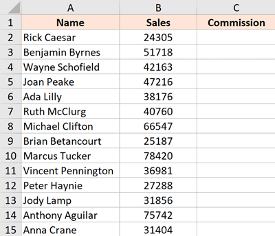
The formula for this would be:
=B2*15%
Below is the way to apply this formula to the entire column C:
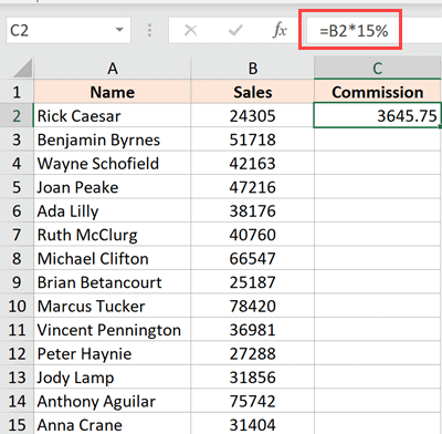
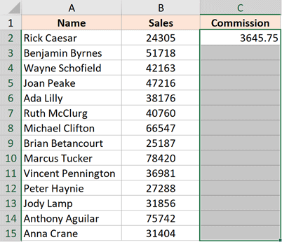
- In cell A2, enter the formula: =B2*15%

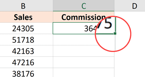
- With the cell selected, you will see a small green square at the bottom-right part of the selection.

- Place the cursor over the small green square. You will notice that the cursor changes to a plus sign (this is called the autofill handle)

- Double click the left mouse key

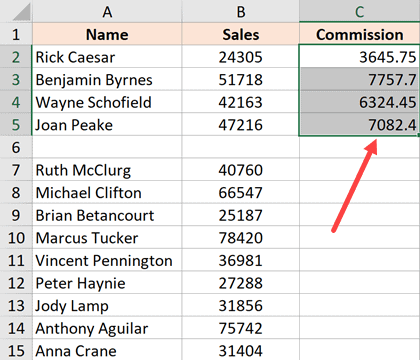
The above steps would automatically fill the entire column till the cell where you have the data in the adjacent column. In our example, the formula would be applied till cell C15
For this to work, there shouldn’t be data in the adjacent column and there should not be any blank cells in it. If, for example, there is a blank cell in column B (say cell B6), then this auto-fill double click would only apply the formula till cell C5
When you use the autofill handle to apply the formula to the entire column, it’s equivalent to copy-pasting the formula manually. This means that the cell reference in the formula would change accordingly.
For example, if it’s an absolute reference, it would remain as is while the formula is applied to the column, add if it’s a relative reference, then it would change as the formula is applied to the cells below.
By Dragging the AutoFill Handle
One issue with the above double click method is that it would stop as soon as it encountered a blank cell in the adjacent columns.
If you have a small data set, you can also manually drag the fill handle to apply the formula in the column.
Below are the steps to do this:
- In cell A2, enter the formula: =B2*15%
- With the cell selected, you will see a small green square at the bottom-right part of the selection
- Place the cursor over the small green square. You will notice that the cursor changes to a plus sign
- Hold the left mouse key and drag it to the cell where you want the formula to be applied
- Leave the mouse key when done
Using the Fill Down Option (it’s in the ribbon)
Another way to apply a formula to the entire column is by using the fill down option in the ribbon.
For this method to work, you first need to select the cells in the column where you want to have the formula.
Below are the steps to use the fill down method:
- In cell A2, enter the formula: =B2*15%
- Select all the cells in which you want to apply the formula (including cell C2)

- Click the Home tab

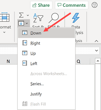
- In the editing group, click on the Fill icon

- Click on ‘Fill down’

The above steps would take the formula from cell C2 and fill it in all the selected cells
Adding the Fill Down in the Quick Access Toolbar
If you need to use the fill down option often, you can add that to the Quick Access Toolbar, so that you can use it with a single click (and it’s always visible on the screen).
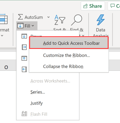
T0 add it to the Quick Access Toolbar (QAT), go to the ‘Fill Down’ option, right-click on it, and then click on ‘Add to the Quick Access Toolbar’
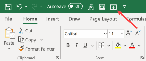
Now, you will see the ‘Fill Down’ icon appear in the QAT.
Using Keyboard Shortcut
If you prefer using the keyboard shortcuts, you can also use the below shortcut to achieve the fill down functionality:
CONTROL + D (hold the control key and then press the D key)
Below are the steps to use the keyboard shortcut to fill-down the formula:
- In cell A2, enter the formula: =B2*15%
- Select all the cells in which you want to apply the formula (including cell C2)
- Hold the Control key and then press the D key
Using Array Formula
If you’re using Microsoft 365 and have access to dynamic arrays, you can also use the array formula method to apply a formula to the entire column.
Suppose you have a data set as shown below and you want to calculate the Commission in column C.
Below is the formula that you can use:
=B2:B15*15%
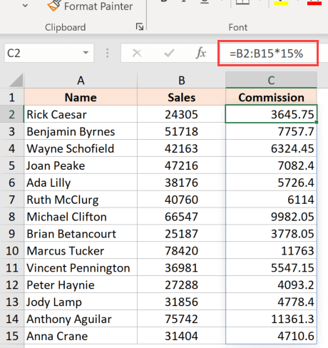
This is an Array formula that would return 14 values in the cell (one each for B2:B15). But since we have dynamic arrays, the result would not be restricted to the single-cell and would spill over to fill the entire column.
Note that you cannot use this formula in every scenario. In this case, because our formula uses the input value from an adjacent column and as the same length of the column in which we want the result (i.e., 14 cells), it works fine here.
But if this is not the case, this may not be the best way to copy a formula to the entire column
By Copy-Pasting the Cell
Another quick and well-known method of applying a formula to the entire column (or selected cells in the entire column) is to simply copy the cell that has the formula and paste it over those cells in the column where you need that formula.
Below are the steps to do this:
- In cell A2, enter the formula: =B2*15%
- Copy the cell (use the keyboard shortcut Control + C in Windows or Command + C in Mac)
- Select all the cells where you want to apply the same formula (excluding cell C2)
- Paste the copied cell (Control + V in Windows and Command + V in Mac)
One difference between this copy-paste method and all the methods convert below above this is that with this method you can choose to only paste the formula (and not paste any of the formattings).
For example, if cell C2 has a blue cell color in it, all the methods covered so far (except the array formula method) would not only copy and paste the formula to the entire column but also paste the formatting (such as the cell color, font size, bold/italics)
If you want to only apply the formula and not the formatting, use the steps below:
- In cell A2, enter the formula: =B2*15%
- Copy the cell (use the keyboard shortcut Control + C in Windows or Command + C in Mac)
- Select all the cells where you want to apply the same formula
- Right-click on the Selection
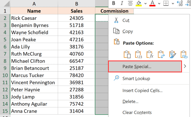
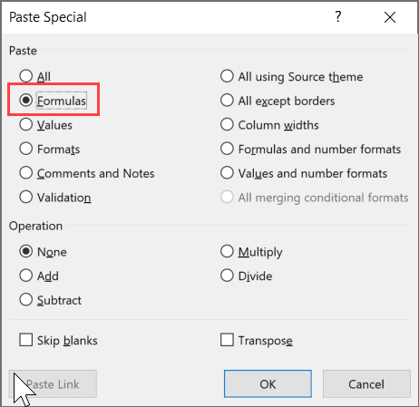
- In the options that appear, click on ‘Paste Special’

- In the ‘Paste Special’ dialog box, click on the Formulas option

- Click OK
The above steps would make sure that only the formula is copied to the selected cells (and none of the formattings comes over with it).
So these are some of the quick and easy methods that you can use to apply a formula to the entire column in Excel.
I hope you found this tutorial useful!
Other Excel tutorials you may also like:
- 5 Ways to Insert New Columns in Excel (including Shortcut & VBA)
- How to Sum a Column in Excel
- How to Compare Two Columns in Excel (for matches & differences)
- Lookup and Return Values in an Entire Row/Column in Excel
- How to Copy and Paste Columns in Excel?
- Apply Conditional Formatting Based on Another Column in Excel
- How to Multiply a Column by a Number in Excel
Transcript
In this video, we’ll look more closely at how calculated columns work in Excel Tables.
One of the best features of tables is called «calculated columns».
Calculated columns help you enter and maintain formulas in Excel tables.
To explain how this works, let me first add a formula to this data, which is not an Excel Table.
A quick way to copy down the formula is to double-click the fill handle.
Since every cell has a price, Excel copies the formula to the bottom.
Next, I’ll add a formula to calculate a 7% tax. Again, I can double-click the fill handle to copy it down.
This works pretty well, but what happens if I change the tax to 8% in the first cell?
At this point, the first formula is out of sync with the rest.
To make sure all formulas are consistent, I need to copy the formula down again.
Now let’s look at the same formulas in an Excel table on the next sheet.
When I enter the Total formula, the formula automatically fills the entire column.
There is no need to copy it down.
The same is true of the Tax formula. After I hit Enter, the formula is copied to the bottom of the column.
Even better, if I edit a formula — for example, if I change the tax rate to 8% — this change is replicated throughout the column automatically.
That’s how calculated columns work.
Notice the autocorrect icon appears when using calculated columns. You can use this menu to navigate directly to Excel’s autocorrect options.
Be aware that if you choose the Stop option, you’re actually turning off the fill formulas setting in Excel.
If you do this, you’ll see your change revert to a local change.
With the setting disabled, you’ll now see a prompt to «overwrite formulas» whenever you make a change to a table column that contains formulas.
This works somewhat like calculated columns but with a manual trigger.
To reenable fill formulas, you’ll need to visit the Auto Format options in the Proofing area.
Excel Tables are very useful in managing and analyzing data in tabular format. An Excel Table provides the data in a special structure, which comes with filtering, formatting, and sizing, and can also auto populate formulas dynamically. In this guide, we’re going to show you how to create calculated columns in Excel tables.
How to Create Calculated Columns in Excel Tables
Follow the steps below to add calculated columns into your Excel Tables. Since you want to add a formula, you may already have an Excel Table. If you don’t have your table yet, please see How to insert an Excel table for more details.
1. Select a cell inside the column
Begin by selecting a cell inside the column you want to add your formulas. It doesn’t matter which row you click on, as long as it is not in the header row.
Tip: You do not need to adjust your table if the new column is adjacent to the table. Excel will expand the table automatically.

2. Enter the formulas
Enter your formulas and press Enter to populate the entire column with your formula. Excel will automatically match the formatting, aggregate calculations, and add or remove any fields as necessary.

3. (Optional) Update the header of the new column
If you add a brand new column without setting a header, Excel will give it a generic name like Column1. Simply click on the header cell and type in the header name you want. This step obviously won’t be necessary if you’re using an existing column for adding formulas.

4. (Optional) Customization
You can now customize your table however you’d like. For more information, please see Tips for Excel Tables

Applying a formula is the most common task, but when we need to apply the same formula in the cells of an entire column, it becomes a tedious task. There are multiple ways to learn how to insert a formula for the entire column.
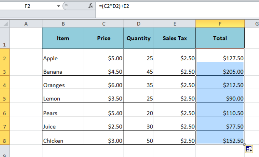 Figure 1. Applying Formula to an Entire Column
Suppose we have a list of items with given price, quantity and sales tax amount and we want to calculate the total amount for each item in column F by using the formula syntax
=(Price * Quantity) + Sales Tax
In cell F2, we apply the formula =(C2*D2)+E2 to calculate Total Amount. There are multiple ways to learn how to apply a formula to an entire column.
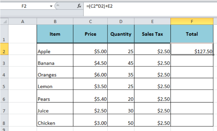 Figure 2. Excel Column Functions
By Dragging the Fill Handle
Once we have entered the formula in row 2 of column F, then we can apply this formula to the entire column F by dragging the Fill handle. Just select the cell F2, place the cursor on the bottom right corner, hold and drag the Fill handle to apply the formula to the entire column in all adjacent cells.
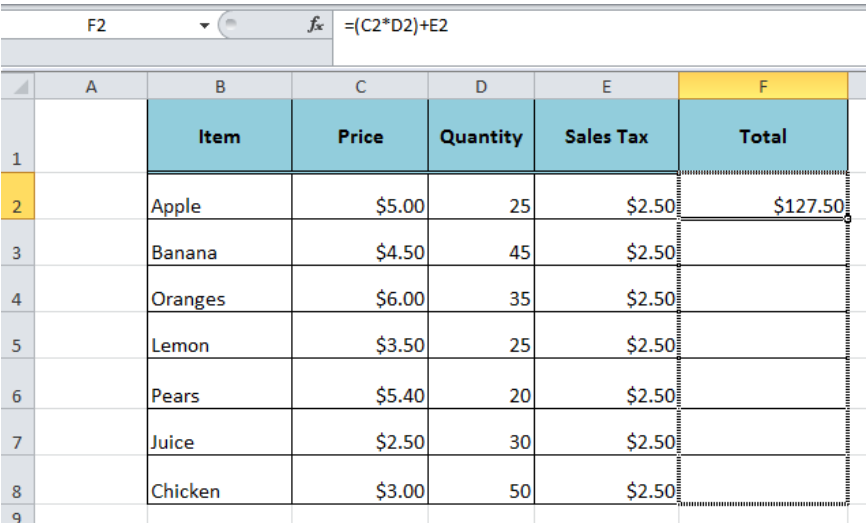 Figure 3. Dragging Fill Handle
By Double-Clicking Fill Handle
The easiest way to apply a formula to the entire column in all adjacent cells is by double-clicking the fill handle by selecting the formula cell. In this example, we need to select the cell F2 and double click on the bottom right corner. Excel applies the same formula to all the adjacent cells in the entire column F.
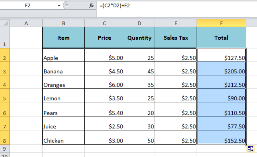 Figure 4. Double Click the Fill Handle
By Using Fill Command
Using Fill command is another good method to apply the formula to an entire column. We need to do the following to achieve for the entire column;
- After entering the formula in cell F2,
- Press Ctrl+Shift+End short keys. This will select the last used cell in the entire column.
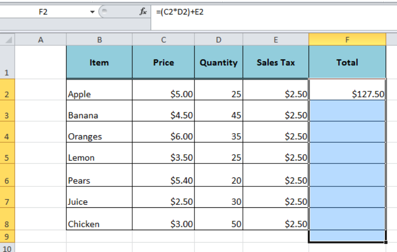 Figure 5. Selecting Last Used Cell in the Entire Column
- Go to Editing Group on Home tab, click in Fill arrow and select DOWN or alternately press Ctrl+D.
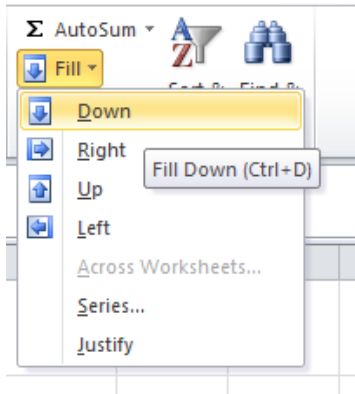 Figure 6. Using Fill Command
- Fill command applies the formula to all the selected cells.
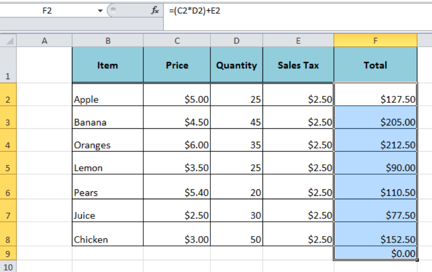 Figure 7. Column Function
Instant Connection to an Expert through our Excelchat Service
Most of the time, the problem you will need to solve will be more complex than a simple application of a formula or function. If you want to save hours of research and frustration, try our live Excelchat service! Our Excel Experts are available 24/7 to answer any Excel question you may have. We guarantee a connection within 30 seconds and a customized solution within 20 minutes.
Содержание
- Считаем сумму в столбце в Экселе
- Способ 1: Просмотр общей суммы
- Способ 2: Автосумма
- Способ 3: Автосумма нескольких столбцов
- Способ 4: Суммирование вручную
- Заключение
- Вопросы и ответы

Основная функциональность Microsoft Excel завязана на формулах, благодаря которым с помощью этого табличного процессора можно не только создать таблицу любой сложности и объема, но и вычислять те или иные значения в ее ячейках. Подсчет суммы в столбце – одна из наиболее простых задач, с которой пользователи сталкиваются чаще всего, и сегодня мы расскажем о различных вариантах ее решения.
Считаем сумму в столбце в Экселе
Посчитать сумму тех или иных значений в столбцах электронной таблицы Excel можно как вручную, так и автоматически, воспользовавшись базовым инструментарием программы. Кроме того, имеется возможность обычного просмотра итогового значения без его записи в ячейку. Как раз с последнего, наиболее простого мы и начнем.
Способ 1: Просмотр общей суммы
Если вам нужно просто увидеть общее значение по столбцу, в ячейках которого содержаться определенные сведения, при этом постоянно держать эту сумму перед глазами и создавать для ее вычисления формулу не требуется, выполните следующее:
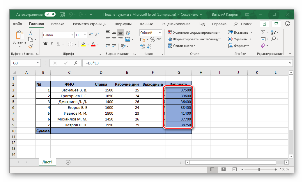
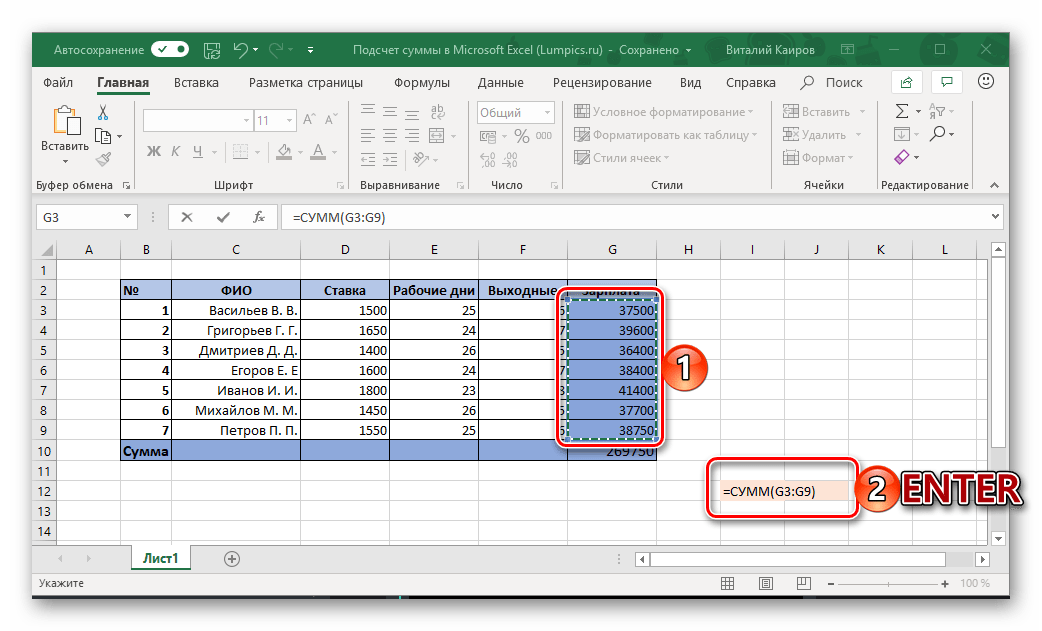
- С помощью мышки выделите диапазон ячеек в столбце, сумму значений в котором требуется посчитать. В нашем примере это будут ячейки с 3 по 9 столбца G.
- Взгляните на строку состояния (нижняя панель программы) – там будет указана искомая сумма. Отображаться это значение будет исключительно до тех пор, пока выделен диапазон ячеек.
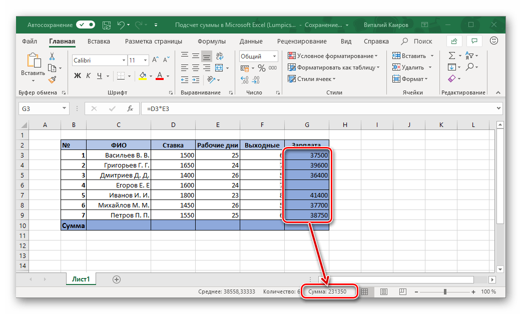
- Дополнительно. Такое суммирование работает, даже если в столбце есть пустые ячейки.

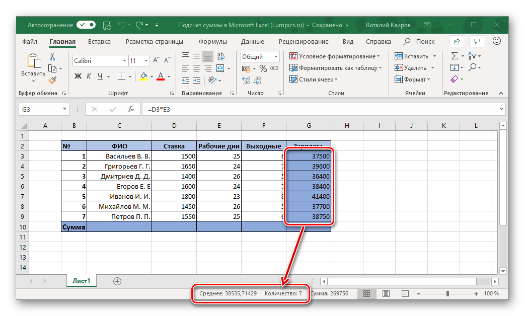
Более того, аналогичным образом можно посчитать сумму всех значений в ячейках сразу из нескольких столбцов – достаточно просто выделить необходимый диапазон и посмотреть на строку состояния. Подробнее о том, как это работает, расскажем в третьем способе данной статьи, но уже на примере шаблонной формулы.
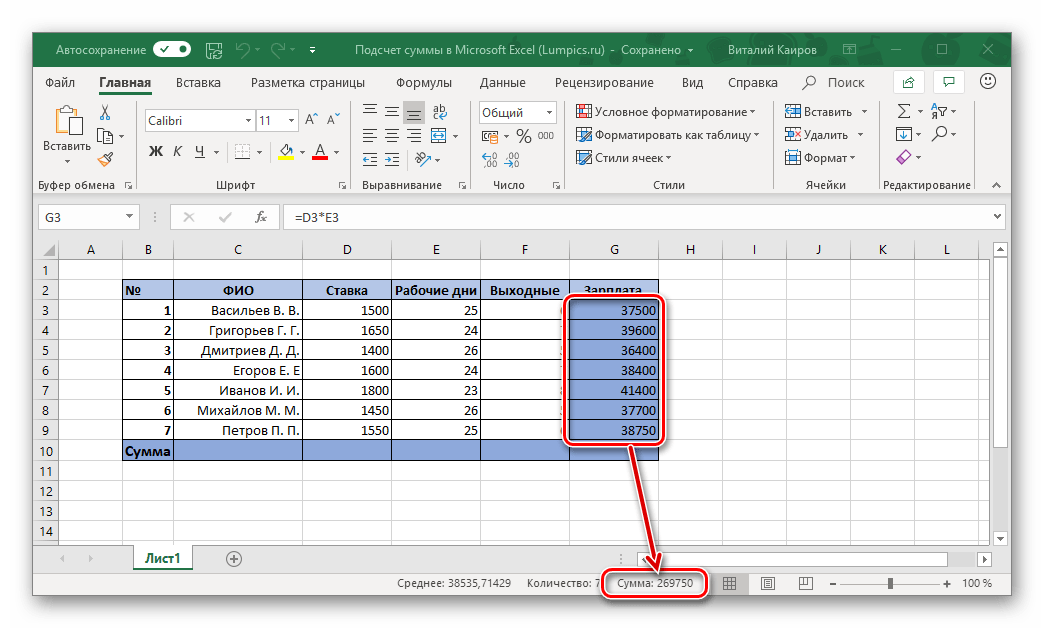
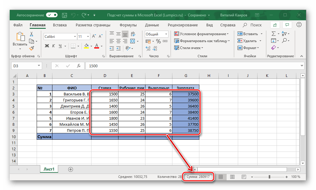
Примечание: Слева от суммы указано количество выделенных ячеек, а также среднее значение для всех указанных в них чисел.
Способ 2: Автосумма
Очевидно, что значительно чаще сумму значений в столбце требуется держать перед глазами, видеть ее в отдельной ячейке и, конечно же, отслеживать изменения, если таковые вносятся в таблицу. Оптимальным решением в таком случае будет автоматическое суммирование, выполняемое с помощью простой формулы.
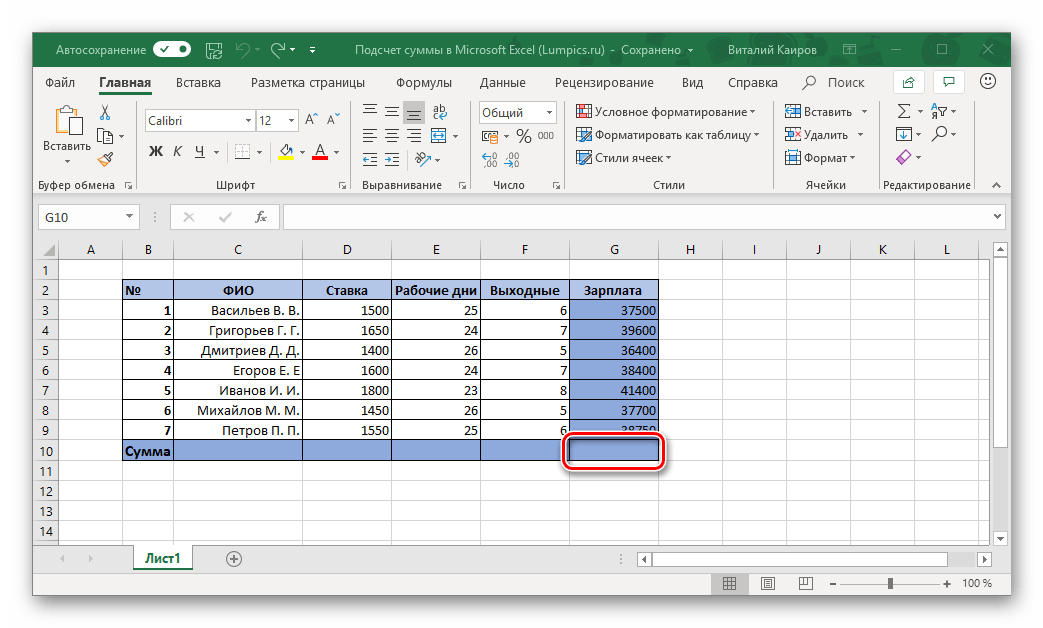
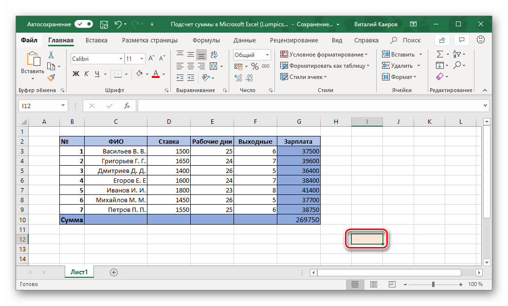
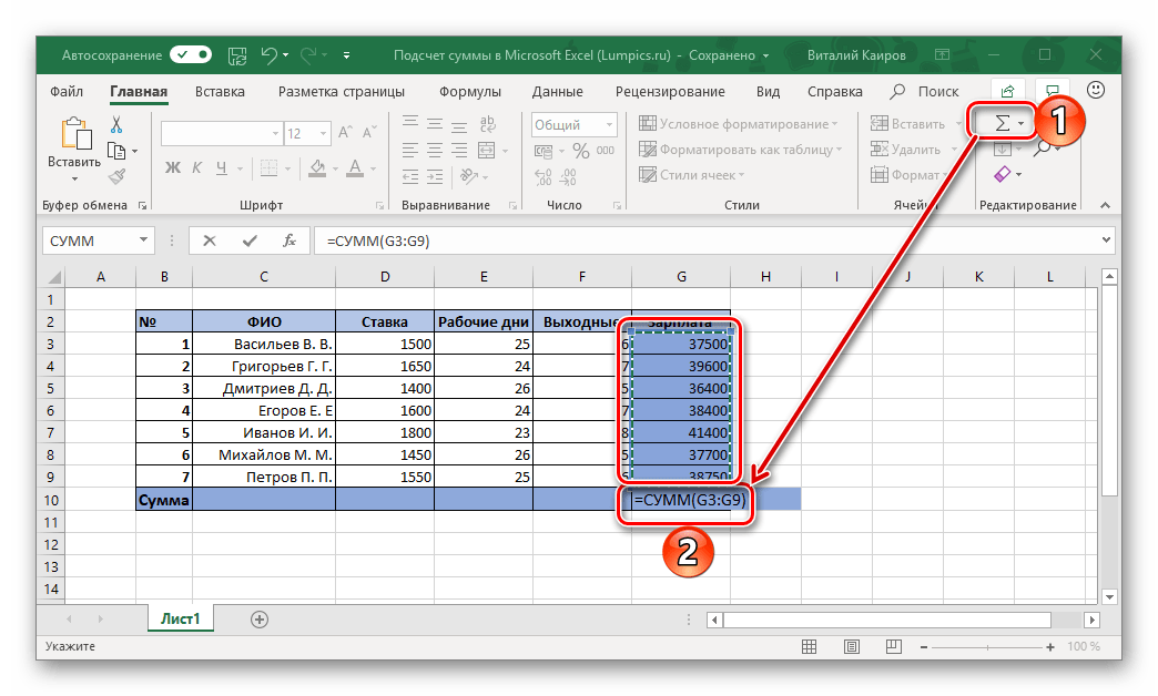
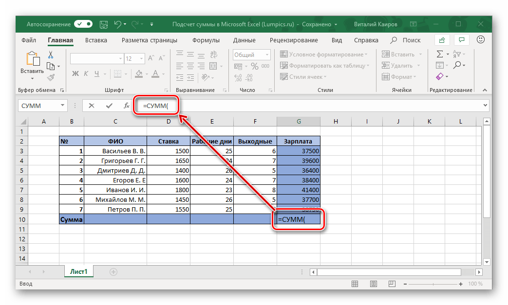
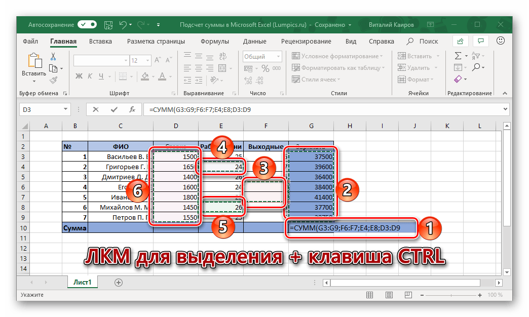
- Нажмите левой кнопкой мышки (ЛКМ) по пустой ячейке, расположенной под теми, сумму которых требуется посчитать.
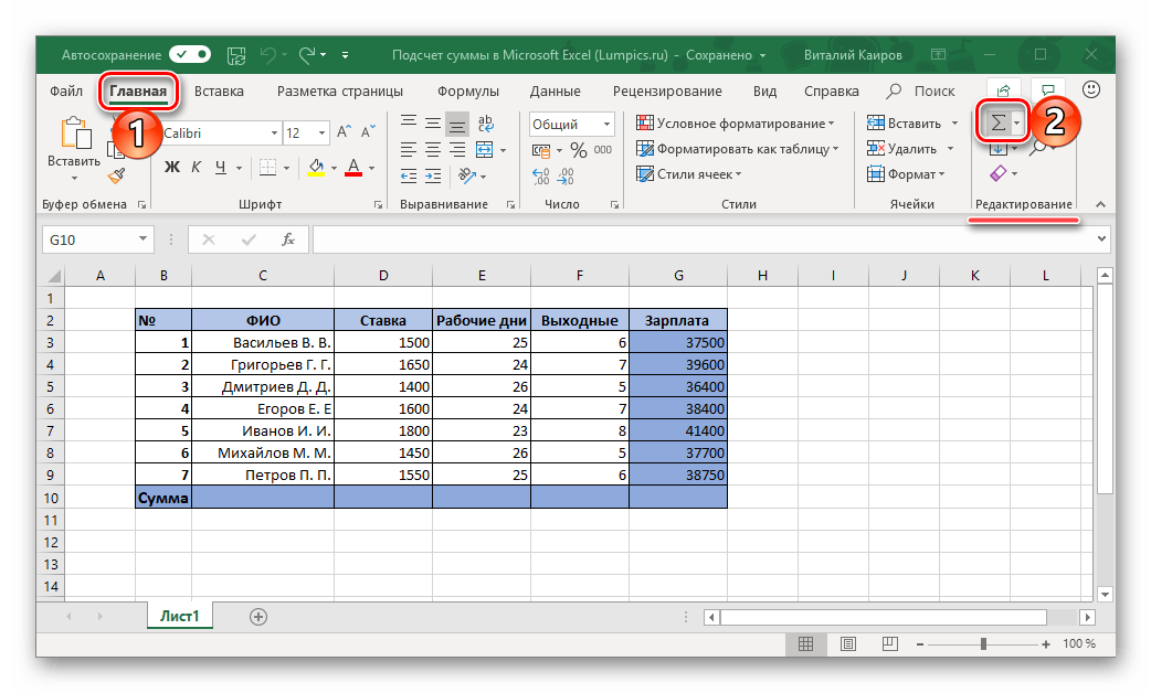
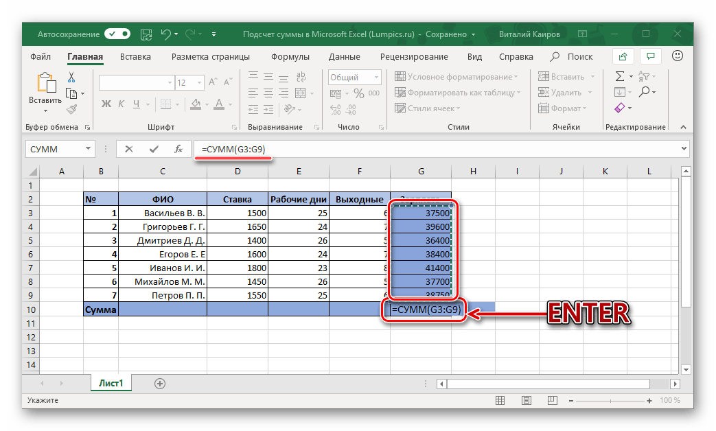
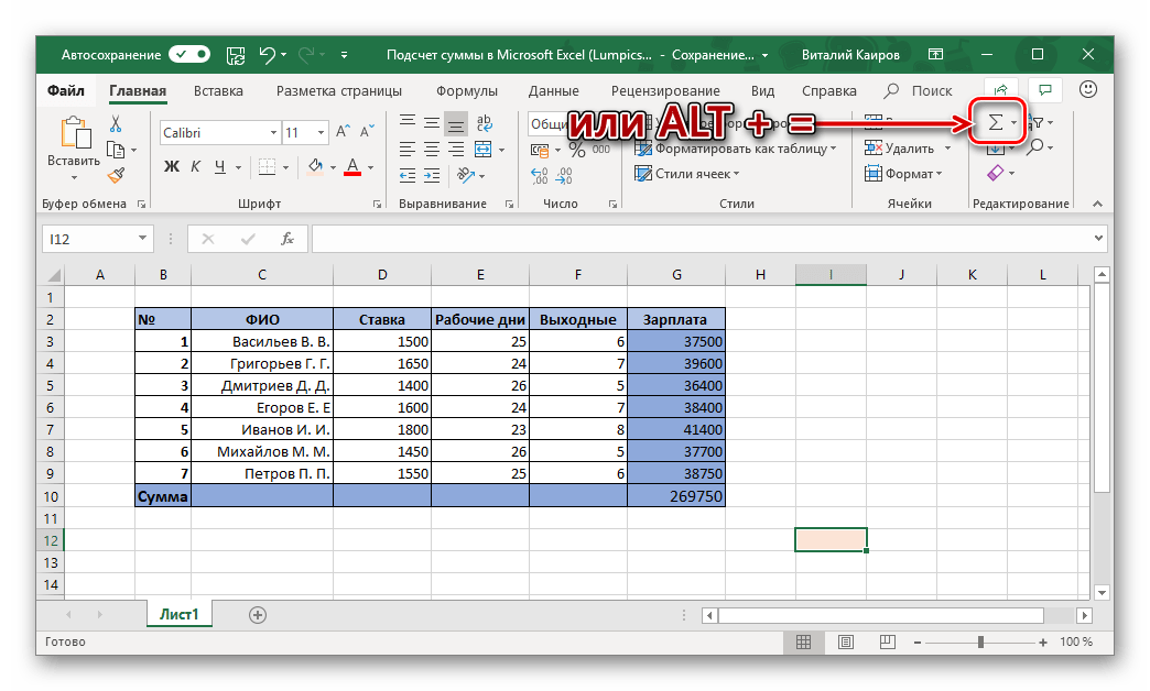
- Кликните ЛКМ по кнопке «Сумма», расположенной в блоке инструментов «Редактирование» (вкладка «Главная»). Вместо этого можно воспользоваться комбинацией клавиш «ALT» + «=».
- Убедитесь, что в формуле, которая появилась в выделенной ячейке и строке формул, указан адрес первой и последней из тех, которые необходимо суммировать, и нажмите «ENTER».
Вы сразу же увидите сумму чисел во всем выделенном диапазоне.
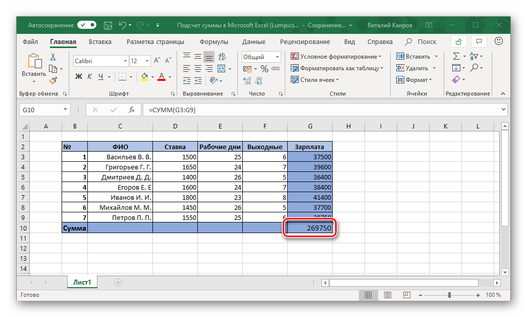
Примечание: Любое изменение в ячейках из выделенного диапазона моментально будет отражаться на итоговой формуле, то есть результат в ней тоже будет меняться.
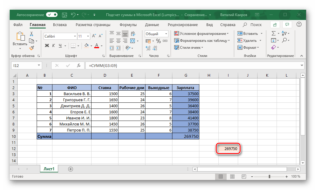
Бывает так, что сумму нужно вывести не в ту ячейку, которая находится под суммируемыми, а в какую-нибудь другую, возможно, расположенную совсем в другом столбце таблицы. В таком случае действовать необходимо следующим образом:
- Выделите кликом ячейку, в которой будет вычисляться сумма значений.
- Нажмите по кнопке «Сумма» или воспользуйтесь горячим клавишам, предназначенным для ввода этой же формулы.
- С помощью мышки выделите диапазон ячеек, которые требуется просуммировать, и нажмите «ENTER».

Совет: Выделить диапазон ячеек можно и немного иным способом – кликните ЛКМ по первой из них, затем зажмите клавишу «SHIFT» и кликните по последней.
Практически точно так же можно суммировать значения сразу из нескольких столбцов или отдельных ячеек, даже если в диапазоне будут пустые ячейки, но обо всем этом далее.
Способ 3: Автосумма нескольких столбцов
Бывает так, что требуется посчитать сумму не в одном, а сразу в нескольких столбцах электронной таблицы Эксель. Делается это практически так же, как и в предыдущем способе, но с одним небольшим нюансом.
- Щелкните ЛКМ по той ячейке, в которую планируете выводить сумму всех значений.
- Нажмите по кнопке «Сумма» на панели инструментов или воспользуйтесь предназначенной для ввода этой формулы комбинацией клавиш.
- Первый столбец (над формулой) уже будет выделен. Поэтому зажмите клавишу «CTRL» на клавиатуре и выделите следующий диапазон ячеек, который тоже должен входить в рассчитываемую сумму.
- Далее, аналогичным образом, если это еще потребуется, зажимая клавишу «CTRL», выделите ячейки из других столбцов, содержимое которых тоже должно входить в итоговую сумму.

Нажмите «ENTER» для подсчета, после чего в предназначенной для формулы ячейке и строке на панели инструментов появится итоговое вычисление.

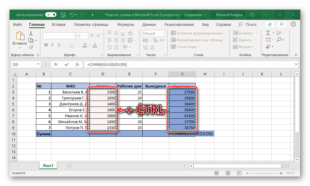
Примечание: Если столбцы, которые требуется посчитать, идут подряд, выделять их можно все вместе.
Несложно догадаться, что аналогичным образом можно посчитать сумму значений в отдельных ячейках, состоящих как в разных столбцах, так и в пределах одного.
Для этого нужно просто выделить кликом ячейку для формулы, нажать по кнопке «Сумма» или на горячие клавиши, выделить первый диапазон ячеек, а затем, зажимая клавишу «CTRL», выделить все остальные «участки» таблицы. Сделав это, просто нажмите «ENTER» для отображения результата.
Как и в предыдущем способе, формула суммы может быть записана в любую из свободных ячеек таблицы, а не только в ту, которая находится под суммируемыми.
Способ 4: Суммирование вручную
Как и любая формула в Microsoft Excel, «Сумма» имеет свой синтаксис, а потому она может быть прописана вручную. Зачем это нужно? Хотя бы за тем, что таким образом вы точно сможете избежать случайных ошибок при выделении суммируемого диапазона и указании входящих в него ячеек. Более того, даже если вы ошибетесь на каком-то из шагов, исправить это будет так же просто, как банальную опечатку в тексте, а значит, не потребуется проделывать всю работу с нуля, как это иногда приходится делать.
Помимо прочего, самостоятельный ввод формулы позволяет разместить ее не только в любом месте таблицы, но и на любом из листов конкретного электронного документа. Стоит ли говорить о том, что таким образом можно просуммировать не только столбцы и/или их диапазоны, но и просто отдельные ячейки или группы таковых, исключая при этом те, которые не должны быть учтены?
Формула суммы имеет следующий синтаксис:
=СУММ(суммируемые ячейки или диапазон таковых)
То есть все то, что должно быть суммировано, записывается в скобки. Значения, указываемые внутри скобок, должны выглядеть следующим образом:
А теперь перейдем непосредственно к ручному суммированию значений в столбце/столбцах электронной таблицы Эксель.
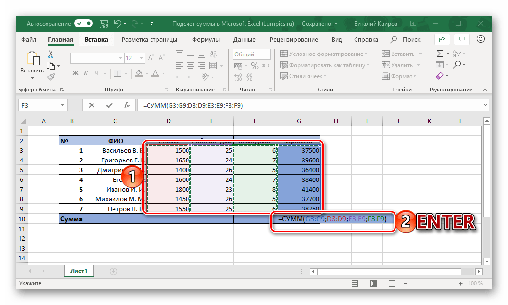
- Выделите нажатием ЛКМ ту ячейку, которая будет содержать итоговую формулу.
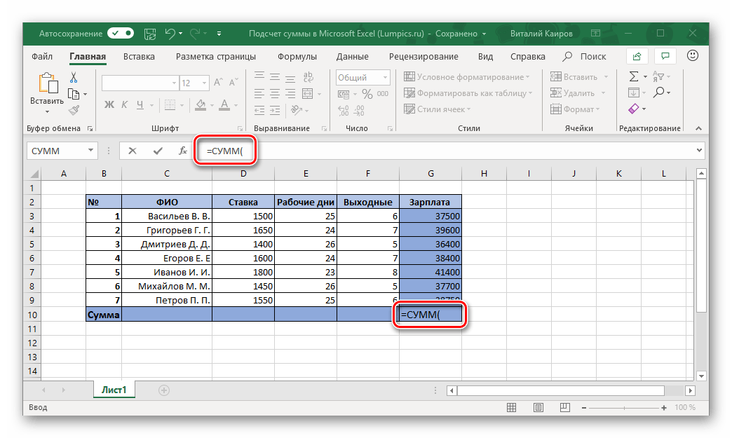
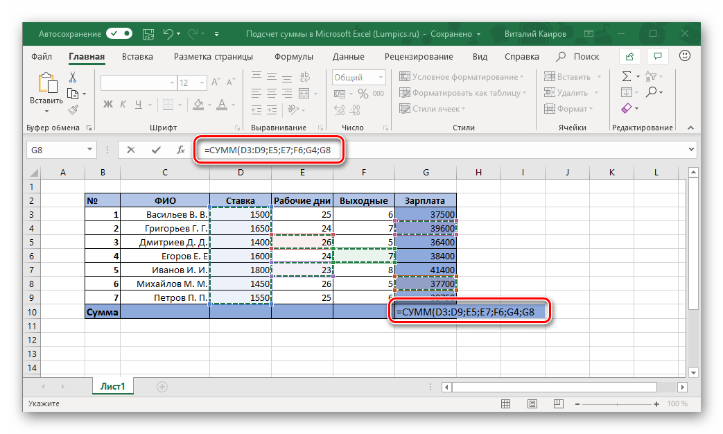
- Введите в нее следующее:
=СУММ(
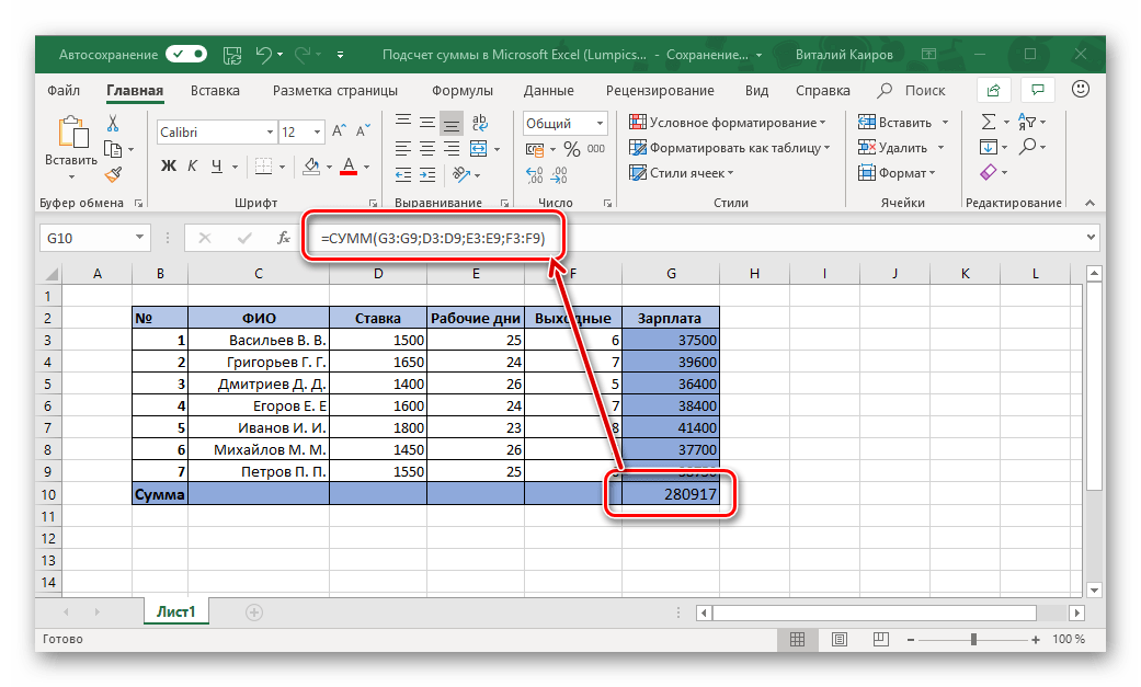
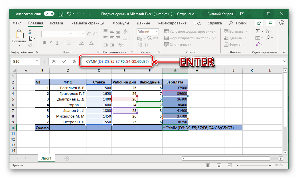
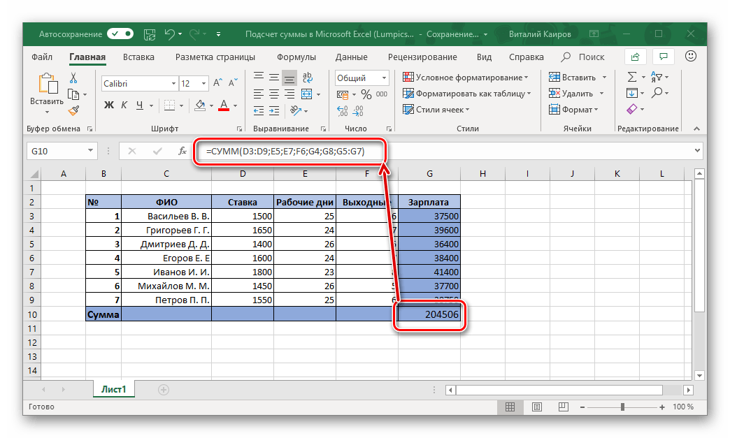
после чего начните поочередно вводить в строке формул адреса суммируемых диапазонов и/или отдельных ячеек, не забывая о разделителях («:» — для диапазона, «;» — для единичных ячеек, вводить без кавычек), то есть делайте все по тому алгоритму, суть которого мы выше подробно описали. - Указав все те элементы, которые требуется просуммировать и убедившись, что вы ничего не пропустили (можно сориентироваться не только по адресам в строке формул, но и по подсветке выделенных ячеек), закройте скобку и нажмите «ENTER» для подсчета.

Примечание: Если вы заметили ошибку в итоговой формуле (например, туда вошла лишняя ячейка или какая-то была пропущена), просто вручную введите правильное обозначение (или удалите лишнее) в строке формул. Аналогичным образом, если и когда это потребуется, можно поступить и с символами-разделителями в виде «;» и «:».

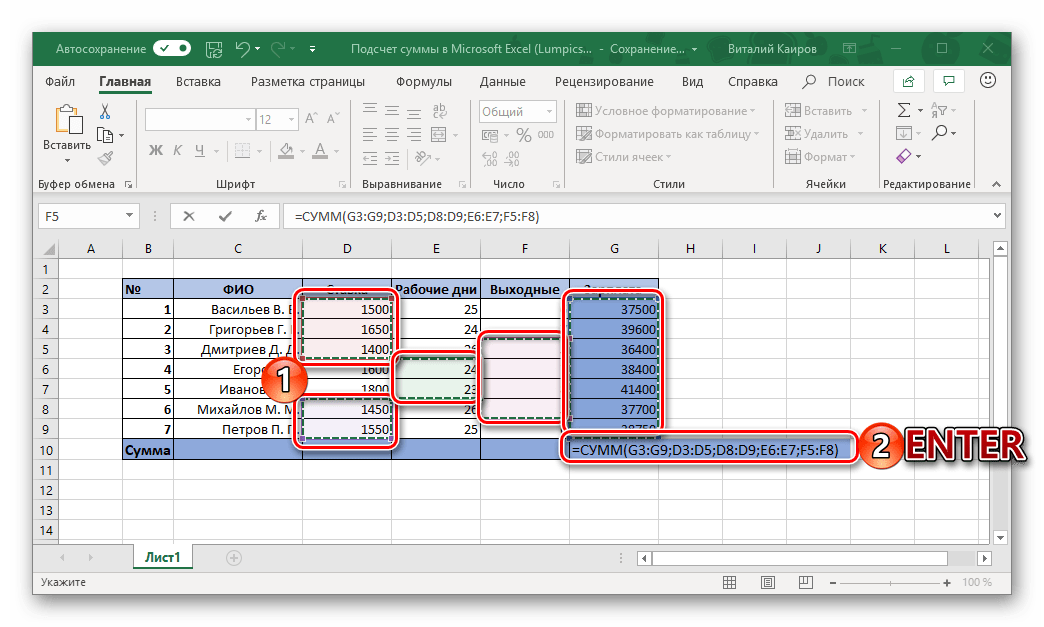
Как вы, наверное, уже могли догадаться, вместо ручного ввода адресов ячеек и их диапазонов можно просто выделять необходимые элементы с помощью мышки. Главное, не забывать при этом удерживать клавишу «CTRL», когда вы переходите от выделения одного элемента к другому.

Самостоятельный, ручной подсчет суммы в столбце/столбцах и/или отдельных ячейках таблицы – задача не самая удобная и быстрая в реализации. Но, как мы уже сказали выше, такой подход предоставляет куда более широкие возможности для взаимодействия со значениями и позволяет моментально исправлять случайные ошибки. А вот то, делать ли это полностью вручную, вводя с клавиатуры в формулу каждую переменную, или использовать для этого мышку и горячие клавиши – решать только вам.
Заключение
Даже такая, казалось бы, простая задача, как подсчет суммы в столбце, решается в табличном процессоре Microsoft Excel сразу несколькими способами, и каждый из них найдет свое применение в той или иной ситуации.
How to Sum a Column in Excel Step-By-Step (2023)
Excel is great at storing and calculating numbers.
The simplest of all mathematical operations is the addition function (summing up numbers). Microsoft Excel offers an in-built function to sum numbers. 😉
And you’d be amazed to see how swift and smooth it gets to sum thousands of numbers in Excel. The guide below explains how to sum columns and rows in Excel.
So continue scrolling and download our free sample workbook here to tag along with the guide.
How to sum a column in Excel
There are two ways how you can quickly sum up a column in Excel.
1. Through the Status Bar
Here’s a column in Excel that contains numbers. Need the sum of this column?

Select the column by clicking on the column header.

Go to the Status Bar at the bottom of Excel (the right side).

Excel displays the sum of all the numbers in the selected column.
This method of summing a column will only suit you if you quickly want to see the sum of a column. As soon as the selection is released, the Sum from the Status bar disappears.
You cannot copy the Sum value from the status bar.
If you do not want the sum of the entire column but only of some cells in the selected column, select those cells only in the same row.
2. Through the SUM function
To formally calculate SUM in Excel, use the SUM function.
1. Activate a cell and write the SUM function as below.
= SUM (A2:A8)

Select the range of all the cells to be summed as the argument of the Sum function.
2. Hit ‘Enter’ to calculate the sum of the said numbers as below.

Pro Tip!
Cut the above process short. Select the cell where you want the sum of numbers to appear.
Use the keyboard shortcut: Alt key + Equal sign key.
Excel would automatically pick the range to be summed. To define a different range, select the cells to be summed manually and hit enter.✌
Add numbers in Excel across rows and columns
Adding numbers across a column is as easy as explained above.
Can we take this the other way around? Adding numbers across rows and columns?
1. Here’s a dense pack of data with numbers and numbers.

2. We want to sum each row and each column of this data.
3. Begin by summing up the first row.
4. Activate the first empty cell where the row ends (or any other cell as you like).
5. Write the SUM formula below in the formula bar.
=SUM (B2:E3)

6. Press Enter to get the sum for this row.

7. Drag and drop it to all rows beneath.

8. Time to sum the columns.
9. Activate the cell immediately next to where the first column ends.
10. Write the SUM function as below.
=SUM(B3:B6)

11. Press Enter to get the sum for this column.

12. Drag and drop it to all the columns to the right.

13. And there you go! All rows and columns are summed up.
That’s how you can add numbers across multiple rows and multiple columns.
How to Autosum in Excel
The sum is one of the most commonly used Excel operations. And so, Excel offers an in-built button to facilitate quick additions in Excel.
1. Activate the cell where you want to perform the sum.
2. Go to Formulas > Function Library > Auto Sum.

3. Click on it to launch the drawer of quick functions.


5. Excel operates the SUM function in the active cell. It automatically selects the range to be summed.

6. If you want to choose a different range, select it to calculate the sum of those cells only.
7. Press Enter to perform the sum as follows.

Pretty straightforward? Huh? 😊
That’s it – Now what?
That’s all about summing up columns and rows in Excel. Until now, we have learned different ways to calculate the sum of a column in Excel (some shortcuts too).
This guide further explains how to calculate the sum of rows and columns and how to use the auto-sum feature of Excel.
SUM is a basic operation, and the SUM function is a very basic tool. However, Microsoft Excel also offers advanced variations of the SUM function. Like the SUMIF and IF functions.
My 30-minute free email course will help you learn these two and the very famous VLOOKUP function in Excel. Sign up now!
Kasper Langmann2023-01-19T12:15:05+00:00
Page load link
Our Comment Policy.
We welcome your comments and questions about this lesson. We don’t welcome spam. Our readers get a lot of value out of the comments and answers on our lessons and spam hurts that experience. Our spam filter is pretty good at stopping bots from posting spam, and our admins are quick to delete spam that does get through. We know that bots don’t read messages like this, but there are people out there who manually post spam. I repeat — we delete all spam, and if we see repeated posts from a given IP address, we’ll block the IP address. So don’t waste your time, or ours. One other point to note — if you post a link in your comment, it will automatically be deleted.
Add a comment to this lesson
.
Comments on this lesson
Very cool
Very nicely worded. I like being able to understand what I’m doing, instead of just copy/pasting
.
Thank you
Fantastic tutorial, I can use excel but had never done a running total, it took me about 30 seconds of reading to understand what to do….far better than microsoft help page!
.
running total amount in excel
The Total Amount is incrementing(single cell:H2) when value is entered in the same cell(G2)..e.g today if you enter in G2 the value of 30 the total amount in H2 is 30;when you enter tomorrow in G2(same cell) the value of 50, the total amount in H2 should be 80;and when you enter again 80 in the same cell(G2)the next day, the total amount should now be 160…hope you could shed a light on this…Thank you very much…
.
Running Total
Thank you for posting this. It worked perfectly.
.
find Cumulative total of column with large vol different items
Month numbers Tno Name PF own PF co cum own cum co
Sep-13 1 335 Mr A 13598.00 13057.00
Oct-13 2 335 Mr A 14099.00 13558.00
Nov-13 3 335 Mr A 14099.00 13558.00
Dec-13 4 335 Mr A 14099.00 13558.00
Jan-14 5 335 Mr A 14099.00 13558.00
Feb-14 6 335 Mr A 14099.00 13558.00
Mar-14 7 335 Mr A 14099.00 13558.00
Sep-13 1 338 Mr B 13598.00 13057.00
Oct-13 2 338 Mr B 14099.00 13558.00
Nov-13 3 338 Mr B 14099.00 13558.00
Dec-13 4 338 Mr B 14099.00 13558.00
Jan-14 5 338 Mr B 14099.00 13558.00
Feb-14 6 338 Mr B 14099.00 13558.00
Mar-14 7 338 Mr B 14099.00 13558.00
.
excel formulas, combinations, etc
thanks. Long, I have been searching for a formula. I could explain the problem too. But, today, I got it. thank you. In future, I may request your help.
.
Complete Column
That works great. It solved my no reference error for the first line, which i need to apply for the whole column (STRG + D).
.
Thanks!
I’m so happy to have a resource like this available to me! I finally figured out how to use the pesky $ sign in my formulas. Thank you internet stranger!
.
Hi I seem to have stumbled
Hi I seem to have stumbled across a problem that I simply can’t find the answer to. I want to have a running total against the days of the month (so a full year would be 365 lines). Income and outgoings, and the total. I can make the sum of two cells as above, but I can’t seem to figure out how to make that cell, for example, D2 carry onto D3/4/5 and only being adjusted by the income and outgoings (B and C). I’d be hugely appreciative if you have a solution, I’m fairly sure it’s an easy one but I simply don’t have any experience with Excel.
.
I think the solution you need is simple
Hi Dan
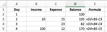
While you could use the approach shown in this lesson, it sounds like you need a simple formula that looks something like this:
=D2+B3-C3
In this formula, I’m assuming the following:
- This formula will be entered into D3
- D2 (the cell above) contains your opening balance. This will need to be manually entered.
- B3 contains Income.
- C3 contains Expenses.
Essentially, this formula says «take the balance from the previous row, add the income for today and subtract the expenses for today». It will be more efficient and therefore faster than a formula that tries to calculate a running balance based on income and expenses, especially as your spreadsheet gets bigger.
You’d then copy and paste this formula down column D to the end of your table.
Here’s an example. Column E shows the formulas from column D:
Some additional thoughts ….
- There’s no reason not to have multiple rows for a given day.
- I’d make sure that there is a column with the number of the day or the actual date.
- Then, you can add multiple rows for each day, and sort them by the day/date column.
This approach is useful for reconciling a bank statement, for example, which can have multiple in/out transactions (or no transactions at all) on a given day
.
You’re right, that formula
You’re right, that formula sounds exactly what it is. Feel a bit silly now for not realising. Thanks millionleaves 
.
Hi
Hi
Do you have the formula that will work, as that just says there is a circular error. I think it’s more like C3:B3 but then I’m stuck. I still can’t get it to take the previous running total into consideration.
.
The formula shown in the image is correct
Hi Dan
The formula in the image that I posted is the correct formula.
If you’re getting a circular error, you may be using a different formula, e.g.
=D3+B3-C3
If you put this formula in D3 it will generate a circular error since it is trying to add itself to itself.
The correct formula in D3 is this:
=D2+B3-C3
Note that the formula in D3 refers to the cell above it — D2 — to get the previous balance.
.
Thanks again, I think I’ve
Thanks again, I think I’ve found it now, it must be my version of Excel or something, it’s this =SUM(D1,B3:C3)
.
Running balance
I’ve started maintaining a bank balance sheet on Excel. There are the debit, credit and balance columns. I have plugged in a formula in the balance column as such: previous balance + debit — credit. It works fine, but I would like to have that formula running down that entire balance column. When I do a Fill Down, it fills the formula in but the value is also there. I would like for the end result to not show up until the row is filled with values. So only when I have a transaction should the balance for that row show up. Thoughts? Thanks.
.
I like how this is going, but…
What I would like to know is if there is a way to get your final result (say D5 in this instance) to just be in one cell instead of the whole column? So it could just sit around E3 or something? It would make the worksheet look more tidy for my needs.
.
won’t calculate zeros
I do a daily total of sales. If there were no sales for the day, and «0.00» is entered into the cell, it puts «0.00 into the subtotal column. I need the total for the last day to populate that days running total. How can I force the system to ignore the zero. I always thought that you just entered a condition like =(IF(C18,1,0))*SUM(C$2:C18) What am I doing wrong. If you could help, I would really appreciate it.
Thank you!
.
Sorted rows running total
How would you get a correct running total for just the rows that are sorted. Ex I need costs of just travel, but main formula is total costs. Lodging, flights, food etc.
.
Sorted rows running total
How would you get a correct running total for just the rows that are sorted. Ex I need costs of just travel, but main formula is total costs. Lodging, flights, food etc.
.
Cumulative formula
I created this one just now =SUM(INDIRECT(«D4:»&»D»&ROW())) — numbers start at D4.
.
Running total
Hi
Looking to create a table of data, that has an accumulative figure for the month. But I want to exclude any data for days that doesn’t meet the required number, in this instance data less than 0. I don’t want a negative number to effect the running total.
Any help for a novice spreadsheet user.
.
Running total
Hi
Looking to create a table of data, that has an accumulative figure for the month. But I want to exclude any data for days that it doesn’t meet a required number, in this instance data less than 0. I don’t want a negative number to effect the running total.
Any help for a novice spreadsheet user.
.
YTD Total Cell
I had to create a paycheck on excel and enter my numbers manually (don’t ask, long story with accountant) and I am wanting a cell to automatically update with the YTD amount if possible.
Currernt YTD
NET PAY $944.28 $944.28 (can i use a formula that would take $944.28 and add the current $ amount automatically? and then next week it would take the Current $ amount and add it again to stay current) or do i have to enter it manually.)
.
Weeks ago i emailed
Weeks ago i emailed Robinsonbuckler (( @yahoo )). com to restore my relationship and he did after 24 hours…
.
Running Total in Table
While this formula works, I run into issues when used in an expandable table. Excel does unexpected things, such as skipping a cell in its calculations. Any advice?
.
cure herpes
I was having Herpes Simplex Virus then i came across a review of people saying that they got treated from Herpes Simplex Virus by Dr Voke., So i gave a try by contacting him through his email and explain my problem to him. He told me all the things I need to do and also give me instructions to take, which I followed properly. Before I knew what is happening after two weeks the HERPES SIMPLEX VIRUS that was in my body got vanished . so if you are also heart broken by any deadly diseases like HERPES HIV, shingles,low sperm count or bringing back your ex lover, this great man is extremely the best in which I have seen and applauds and if you also need a help, you can also email him via email doctorvoke @gmail .com
.
Anna
if you enter in G2 the value of 30 the total amount in H2 is 30;when you enter tomorrow in G2(same cell) the value of 50, the total amount in H2 should be 80;and when you enter again 80 in the same cell(G2)the next day, the total amount should now be 160…hope you could shed a light on this…Thank you very much…
.
Herpes cure
Was cured from herpes virus. thanks to R.buckler 11 [at] G mail com………………..
.
HERPES CURE
I was browsing the Internet searching for help when I came across a testimony shared by someone on how she was cured from Herpes Disease. I quickly contacted him to get the cure. I bought the herbal medicine from the herbal doctor [Robinson Buckler]. I took the herbal medicine for 2 weeks as instructed and i went for a medical checkup and to my greatest surprise i was cured from Herpes virus. My heart is so filled with joy. If you are suffering from Herpes or any other disease you can contact this herbal doctor today on this Email address_________________robinsonbuckler @[[yahoo .com]]…..Thank you Doctor
Robin Burroughs
Denton Avenue
Cookeville, TN 38501
USA
.
.
.
.
Как суммировать числа в столбце Excel
17.03.2017

Многие пользователи знают о табличном процессоре Excel. Кто-то устанавливал его просто для открытия таблиц, а кто-то – для их составления. Часто во время внесения в таблицу данных может понадобиться калькулятор, чтобы посчитать немаленькие числа. Так что для экономии нашего времени функция суммирования (вычитания, умножения и вычитания) была встроена в Эксель. Однако не все знают, как применять её. Именно об этом и будет идти речь в статье.
Как посчитать сумму в столбце
На самом деле, способов для суммирования чисел в столбце несколько, и все мы подробно рассмотрим. Но для начала возьмём любую таблицу для примера.

Способ 1: Ввод ячеек
- Итак, в конце необходимого столбца выделяем ячейку, где нужно вывести сумму чисел. В ней вводим символ «=» («Равно», без кавычек). После него пишем любую ячейку данного столбца, значок «+», ячейку, «+», ячейку и так далее. Сначала пишется заглавная буква ячейки, а потом цифра. Если всё правильно, то цвет надписей будет меняться, а ячейки – выделяться.
- Теперь нажимаем на клавишу «Enter», и результат будет представлен в виде суммы.


Способ 2: Выделение столбца
Этот способ напоминает предыдущий. Но этот будет намного проще, так как вводиться формула будет сама.
- Точно также мы выделяем ячейку под столбцом и пишем знак «=». Теперь нажимаем на верхнюю ячейку и зажимаем левую кнопку мыши. После этого растягиваем появившуюся рамочку до конца столбца.
- Можно заметить, что появилась формула. Перед ней пишем слово «Сумм» и отделяем скобкой.
Нажимаем «Enter» и сумма подсчитана.


Способ 3: Отдел «Автосумма»
Этот способ отличается от всех остальных, так как здесь нужно будет обращаться к панели быстрого доступа.
- На панели инструментов находим отдел «Формулы» и переключаемся на него. Там заходим в меню «Автосумма». В нём кликаем по кнопке «Сумма».
- Как только Вы туда нажали, сразу же заполнится ячейка под столбцом. У неё будет такой же вид, как был в конце выполнения второго способа. Если нажать на «Enter», то посчитается сумма.


Способ 4: Функция «СУММЕСЛИ»
Ещё одна вспомогательная функция, с помощью которой можно задать условия суммирования.
- Заходим в отдел «Формулы» и нажимаем на «Автосумма». Теперь мы выбираем кнопку «Другие функции…».
- Появится новое диалоговое окно, где необходимо найти и выбрать интересующую нас функцию «СУММЕСЛИ». После выбора нажимаем на кнопку «ОК».
- Появится следующие окно под названием «Аргументы функции». Здесь мы указываем диапазон суммирования. То есть, прописываем начальную ячейку, знак «:» и последнюю ячейку. Под этой строкой находится следующая – «Критерии». Здесь можно указать интересующие нас критерии суммирования. Это поле обязательно, так что мы его пропустить не сможем. Иначе сумма не будет подсчитана. Так как нам необходима лишь она, и ничего более, то пишем элементарный критерий – >0 (Больше нуля). Кликаем по кнопке «ОК», и сумма Будет подсчитана.
- Если Вы написали критерий неправильно, то будет либо число «0», либо ошибка.


Теперь Вы узнали о таких возможностях табличного процессора Excel, как суммирование чисел в столбце. Эти знания можно будет применять во время составления протоколов и отчётов, и при вводе обычных данных.