
Содержание
- Excel performance: Improving calculation performance
- The importance of calculation speed
- Understanding calculation methods in Excel
- Full calculation and recalculation dependencies
- Calculation process
- Calculating workbooks, worksheets, and ranges
- Calculate all open workbooks
- Calculate selected worksheets
- Calculate a range of cells
- Volatile functions
- Volatile actions
- Formula and name evaluation circumstances
- Data tables
- Controlling calculation options
- Automatic calculation
- Manual calculation
- Iteration settings
- Workbook ForceFullCalculation property
- Making workbooks calculate faster
- Processor speed and multiple cores
- Measuring calculation time
- Finding and prioritizing calculation obstructions
- Drill-down approach to finding obstructions
- To find obstructions using the drill-down approach
- Speeding up calculations and reducing obstructions
- First rule: Remove duplicated, repeated, and unnecessary calculations
- Second rule: Use the most efficient function possible
- Third rule: Make good use of smart recalculation and multithreaded calculation
- Fourth rule: Time and test each change
- Rule examples
- Period-to-date sums
- Error handling
- Dynamic count unique
- Conclusion
- See also
- Support and feedback
Excel performance: Improving calculation performance
Applies to: Excel | Excel 2013 | Excel 2016 | VBA
The «Big Grid» of 1 million rows and 16,000 columns in Office Excel 2016, together with many other limit increases, greatly increases the size of worksheets that you can build compared to earlier versions of Excel. A single worksheet in Excel can now contain over 1,000 times as many cells as earlier versions.
In earlier versions of Excel, many people created slow-calculating worksheets, and larger worksheets usually calculate more slowly than smaller ones. With the introduction of the «Big Grid» in Excel 2007, performance really matters. Slow calculation and data manipulation tasks such as sorting and filtering make it more difficult for users to concentrate on the task at hand, and lack of concentration increases errors.
Recent Excel versions introduced several features to help you handle this capacity increase, such as the ability to use more than one processor at a time for calculations and common data set operations like refresh, sorting, and opening workbooks. Multithreaded calculation can substantially reduce worksheet calculation time. However, the most important factor that influences Excel calculation speed is still the way your worksheet is designed and built.
You can modify most slow-calculating worksheets to calculate tens, hundreds, or even thousands of times faster. By identifying, measuring, and then improving the calculation obstructions in your worksheets, you can speed up calculation.
The importance of calculation speed
Poor calculation speed affects productivity and increases user error. User productivity and the ability to focus on a task deteriorates as response time lengthens.
Excel has two main calculation modes that let you control when calculation occurs:
Automatic calculation — Formulas are automatically recalculated when you make a change.
Manual calculation — Formulas are recalculated only when you request it (for example, by pressing F9).
For calculation times of less than about a tenth of a second, users feel that the system is responding instantly. They can use automatic calculation even when they enter data.
Between a tenth of a second and one second, users can successfully keep a train of thought going, although they will notice the response time delay.
As calculation time increases (usually between 1 and 10 seconds), users must switch to manual calculation when they enter data. User errors and annoyance levels start to increase, especially for repetitive tasks, and it becomes difficult to maintain a train of thought.
For calculation times greater than 10 seconds, users become impatient and usually switch to other tasks while they wait. This can cause problems when the calculation is one of a sequence of tasks and the user loses track.
Understanding calculation methods in Excel
To improve the calculation performance in Excel, you must understand both the available calculation methods and how to control them.
Full calculation and recalculation dependencies
The smart recalculation engine in Excel tries to minimize calculation time by continuously tracking both the precedents and dependencies for each formula (the cells referenced by the formula) and any changes that were made since the last calculation. At the next recalculation, Excel recalculates only the following:
Cells, formulas, values, or names that have changed or are flagged as needing recalculation.
Cells dependent on other cells, formulas, names, or values that need recalculation.
Volatile functions and visible conditional formats.
Excel continues calculating cells that depend on previously calculated cells even if the value of the previously calculated cell does not change when it is calculated.
Because you change only part of the input data or a few formulas between calculations in most cases, this smart recalculation usually takes only a fraction of the time that a full calculation of all the formulas would take.
In manual calculation mode, you can trigger this smart recalculation by pressing F9. You can force a full calculation of all the formulas by pressing Ctrl+Alt+F9, or you can force a complete rebuild of the dependencies and a full calculation by pressing Shift+Ctrl+Alt+F9.
Calculation process
Excel formulas that reference other cells can be put before or after the referenced cells (forward referencing or backward referencing). This is because Excel does not calculate cells in a fixed order, or by row or column. Instead, Excel dynamically determines the calculation sequence based on a list of all the formulas to calculate (the calculation chain) and the dependency information about each formula.
Excel has distinct calculation phases:
Build the initial calculation chain and determine where to begin calculating. This phase occurs when the workbook is loaded into memory.
Track dependencies, flag cells as uncalculated, and update the calculation chain. This phase executes at each cell entry or change, even in manual calculation mode. Ordinarily this executes so fast that you don’t notice it, but in complex cases, response can be slow.
Calculate all formulas. As a part of the calculation process, Excel reorders and restructures the calculation chain to optimize future recalculations.
Update the visible parts of the Excel windows.
The third phase executes at each calculation or recalculation. Excel tries to calculate each formula in the calculation chain in turn, but if a formula depends on one or more formulas that have not yet been calculated, the formula is sent down the chain to be calculated again later. This means that a formula can be calculated multiple times per recalculation.
The second time that you calculate a workbook is often significantly faster than the first time. This occurs for several reasons:
Excel usually recalculates only cells that have changed, and their dependents.
Excel stores and reuses the most recent calculation sequence so that it can save most of the time used to determine the calculation sequence.
With multiple core computers, Excel tries to optimize the way the calculations are spread across the cores based on the results of the previous calculation.
In an Excel session, both Windows and Excel cache recently used data and programs for faster access.
Calculating workbooks, worksheets, and ranges
You can control what is calculated by using the different Excel calculation methods.
Calculate all open workbooks
Each recalculation and full calculation calculates all the workbooks that are currently open, resolves any dependencies within and between workbooks and worksheets, and resets all previously uncalculated (dirty) cells as calculated.
Calculate selected worksheets
You can also recalculate only the selected worksheets by using Shift+F9. This does not resolve any dependencies between worksheets, and does not reset dirty cells as calculated.
Calculate a range of cells
Excel also allows for the calculation of a range of cells by using the Visual Basic for Applications (VBA) methods Range.CalculateRowMajorOrder and Range.Calculate:
Range.CalculateRowMajorOrder calculates the range left to right and top to bottom, ignoring all dependencies.
Range.Calculate calculates the range resolving all dependencies within the range.
Because CalculateRowMajorOrder does not resolve any dependencies within the range that is being calculated, it is usually significantly faster than Range.Calculate. However, it should be used with care because it may not give the same results as Range.Calculate.
Range.Calculate is one of the most useful tools in Excel for performance optimization because you can use it to time and compare the calculation speed of different formulas.
Volatile functions
A volatile function is always recalculated at each recalculation even if it does not seem to have any changed precedents. Using many volatile functions slows down each recalculation, but it makes no difference to a full calculation. You can make a user-defined function volatile by including Application.Volatile in the function code.
Some of the built-in functions in Excel are obviously volatile: RAND(), NOW(), TODAY(). Others are less obviously volatile: OFFSET(), CELL(), INDIRECT(), INFO().
Some functions that have previously been documented as volatile are not in fact volatile: INDEX(), ROWS(), COLUMNS(), AREAS().
Volatile actions
Volatile actions are actions that trigger a recalculation, and include the following:
- Clicking a row or column divider when in automatic mode.
- Inserting or deleting rows, columns, or cells on a sheet.
- Adding, changing, or deleting defined names.
- Renaming worksheets or changing worksheet position when in automatic mode.
- Filtering, hiding, or un-hiding rows.
- Opening a workbook when in automatic mode. If the workbook was last calculated by a different version of Excel, opening the workbook usually results in a full calculation.
- Saving a workbook in manual mode if the Calculate before Save option is selected.
Formula and name evaluation circumstances
A formula or part of a formula is immediately evaluated (calculated), even in manual calculation mode, when you do one of the following:
- Enter or edit the formula.
- Enter or edit the formula by using the Function Wizard.
- Enter the formula as an argument in the Function Wizard.
- Select the formula in the formula bar and press F9 (press Esc to undo and revert to the formula), or click Evaluate Formula.
A formula is flagged as uncalculated when it refers to (depends on) a cell or formula that has one of these conditions:
- It was entered.
- It was changed.
- It’s in an AutoFilter list, and the criteria drop-down list was enabled.
- It’s flagged as uncalculated.
A formula that is flagged as uncalculated is evaluated when the worksheet, workbook, or Excel instance that contains it is calculated or recalculated.
The circumstances that cause a defined name to be evaluated differ from those for a formula in a cell:
- A defined name is evaluated every time that a formula that refers to it is evaluated so that using a name in multiple formulas can cause the name to be evaluated multiple times.
- Names that are not referred to by any formula are not calculated even by a full calculation.
Data tables
Excel data tables (Data tab > Data Tools group > What-If Analysis > Data Table) should not be confused with the table feature (Home tab > Styles group > Format as Table, or, Insert tab > Tables group > Table). Excel data tables do multiple recalculations of the workbook, each driven by the different values in the table. Excel first calculates the workbook normally. For each pair of row and column values, it then substitutes the values, does a single-threaded recalculation, and stores the results in the data table.
Data table recalculation always uses only a single processor.
Data tables give you a convenient way to calculate multiple variations and view and compare the results of the variations. Use the Automatic except Tables calculation option to stop Excel from automatically triggering the multiple calculations at each calculation, but still calculate all dependent formulas except tables.
Controlling calculation options
Excel has a range of options that enable you to control the way it calculates. You can change the most frequently used options in Excel by using the Calculation group on the Formulas tab on the Ribbon.
Figure 1. Calculation group on the Formulas tab
To see more Excel calculation options, on the File tab, click Options. In the Excel Options dialog box, click the Formulas tab.
Figure 2. Calculation options on the Formulas tab in Excel Options
Many calculation options (Automatic, Automatic except for data tables, Manual, Recalculate workbook before saving) and the iteration settings (Enable iterative calculation, Maximum Iterations, Maximum Change) operate at the application level instead of at the workbook level (they are the same for all open workbooks).
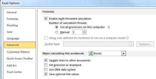
To find advanced calculation options, on the File tab, click Options. In the Excel Options dialog box, click Advanced. Under the Formulas section, set calculation options.
Figure 3. Advanced calculation options
When you start Excel, or when it is running without any workbooks open, the initial calculation mode and iteration settings are set from the first non-template, non-add-in workbook that you open. This means that the calculation settings in workbooks opened later are ignored, although, of course, you can manually change the settings in Excel at any time. When you save a workbook, the current calculation settings are stored in the workbook.
Automatic calculation
Automatic calculation mode means that Excel automatically recalculates all open workbooks at every change and when you open a workbook. Usually when you open a workbook in automatic mode and Excel recalculates, you don’t see the recalculation because nothing has changed since the workbook was saved.
You might notice this calculation when you open a workbook in a later version of Excel than you used the last time that the workbook was calculated (for example, Excel 2016 versus Excel 2013). Because the Excel calculation engines are different, Excel performs a full calculation when it opens a workbook that was saved using an earlier version of Excel.
Manual calculation
Manual calculation mode means that Excel recalculates all open workbooks only when you request it by pressing F9 or Ctrl+Alt+F9, or when you save a workbook. For workbooks that take more than a fraction of a second to recalculate, you must set calculation to manual mode to avoid a delay when you make changes.
Excel tells you when a workbook in manual mode needs recalculation by displaying Calculate in the status bar. The status bar also displays Calculate if your workbook contains circular references and the iteration option is selected.
Iteration settings
If you have intentional circular references in your workbook, the iteration settings enable you to control the maximum number of times the workbook is recalculated (iterations) and the convergence criteria (maximum change: when to stop). Clear the iteration box so that if you have accidental circular references, Excel will warn you and will not try to solve them.
Workbook ForceFullCalculation property
When you set this workbook property to True, Excel’s Smart Recalculation is turned off and every recalculation recalculates all the formulas in all the open workbooks. For some complex workbooks, the time taken to build and maintain the dependency trees needed for Smart Recalculation is larger than the time saved by Smart Recalculation.
If your workbook takes an excessively long time to open, or making small changes takes a long time even in manual calculation mode, it may be worth trying ForceFullCalculation.
Calculate will appear in the status bar if the workbook ForceFullCalculation property has been set to True.
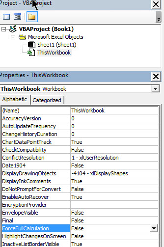
You can control this setting using the VBE (Alt+F11), selecting ThisWorkbook in the Project Explorer (Ctrl+R) and showing the Properties Window (F4).
Figure 4. Setting the Workbook.ForceFullCalculation property
Making workbooks calculate faster
Use the following steps and methods to make your workbooks calculate faster.
Processor speed and multiple cores
For most versions of Excel, a faster processor will, of course, enable faster Excel calculation. The multithreaded calculation engine introduced in Excel 2007 enables Excel to make excellent use of multiprocessor systems, and you can expect significant performance gains with most workbooks.
For most large workbooks, the calculation performance gains from multiple processors scale almost linearly with the number of physical processors. However, hyper-threading of physical processors only produces a small performance gain.
Paging to a virtual-memory paging file is slow. You must have enough physical RAM for the operating system, Excel, and your workbooks. If you have more than occasional hard disk activity during calculation, and you are not running user-defined functions that trigger disk activity, you need more RAM.
As mentioned, recent versions of Excel can make effective use of large amounts of memory, and the 32-bit version of Excel 2007 and Excel 2010 can handle a single workbook or a combination of workbooks using up to 2 GB of memory.
The 32-bit versions of Excel 2013 and Excel 2016 that use the Large Address Aware (LAA) feature can use up to 3 or 4 GB of memory, depending on the version of Windows installed. The 64-bit version of Excel can handle larger workbooks. For more information, see the «Large data sets, LAA, and 64-bit Excel» section in Excel performance: Performance and limit improvements.
A rough guideline for efficient calculation is to have enough RAM to hold the largest set of workbooks that you need to have open at the same time, plus 1 to 2 GB for Excel and the operating system, plus additional RAM for any other running applications.
Measuring calculation time
To make workbooks calculate faster, you must be able to accurately measure calculation time. You need a timer that is faster and more accurate than the VBA Time function. The MICROTIMER() function shown in the following code example uses Windows API calls to the system high-resolution timer. It can measure time intervals down to small numbers of microseconds. Be aware that because Windows is a multitasking operating system, and because the second time that you calculate something, it may be faster than the first time, the times that you get usually don’t repeat exactly. To achieve the best accuracy, measure time calculation tasks several times and average the results.
For more information about how the Visual Basic Editor can significantly affect VBA user-defined function performance, see the «Faster VBA user-defined functions» section in Excel performance: Tips for optimizing performance obstructions.
To measure calculation time, you must call the appropriate calculation method. These subroutines give you calculation time for a range, recalculation time for a sheet or all open workbooks, or full calculation time for all open workbooks.
Copy all these subroutines and functions into a standard VBA module. To open the VBA editor, press Alt+F11. On the Insert menu, select Module, and then copy the code into the module.
To run the subroutines in Excel, press Alt+F8. Select the subroutine you want, and then click Run.
Figure 5. The Excel Macro window showing the calculation timers

Finding and prioritizing calculation obstructions
Most slow-calculating workbooks have only a few problem areas or obstructions that consume most of the calculation time. If you don’t already know where they are, use the drill-down approach outlined in this section to find them. If you do know where they are, you must measure the calculation time that is used by each obstruction so that you can prioritize your work to remove them.
Drill-down approach to finding obstructions
The drill-down approach starts by timing the calculation of the workbook, the calculation of each worksheet, and the blocks of formulas on slow-calculating sheets. Do each step in order and note the calculation times.
To find obstructions using the drill-down approach
Ensure that you have only one workbook open and no other tasks are running.
Set calculation to manual.
Make a backup copy of the workbook.
Open the workbook that contains the Calculation Timers macros, or add them to the workbook.
Check the used range by pressing Ctrl+End on each worksheet in turn.
This shows where the last used cell is. If this is beyond where you expect it to be, consider deleting the excess columns and rows and saving the workbook. For more information, see the «Minimizing the used range» section in Excel performance: Tips for optimizing performance obstructions.
Run the FullCalcTimer macro.
The time to calculate all the formulas in the workbook is usually the worst-case time.
Run the RecalcTimer macro.
A recalculation immediately after a full calculation usually gives you the best-case time.
Calculate workbook volatility as the ratio of recalculation time to full calculation time.
This measures the extent to which volatile formulas and the evaluation of the calculation chain are obstructions.
Activate each sheet and run the SheetTimer macro in turn.
Because you just recalculated the workbook, this gives you the recalculate time for each worksheet. This should enable you to determine which ones are the problem worksheets.
Run the RangeTimer macro on selected blocks of formulas.
For each problem worksheet, divide the columns or rows into a small number of blocks.
Select each block in turn, and then run the RangeTimer macro on the block.
If necessary, drill down further by subdividing each block into a smaller number of blocks.
Prioritize the obstructions.
Speeding up calculations and reducing obstructions
It’s not the number of formulas or the size of a workbook that consumes the calculation time. It’s the number of cell references and calculation operations, and the efficiency of the functions being used.
Because most worksheets are constructed by copying formulas that contain a mixture of absolute and relative references, they usually contain a large number of formulas that contain repeated or duplicated calculations and references.
Avoid complex mega-formulas and array formulas. In general, it is better to have more rows and columns and fewer complex calculations. This gives both the smart recalculation and the multithreaded calculation in Excel a better opportunity to optimize the calculations. It’s also easier to understand and debug. The following are a few rules to help you speed up workbook calculations.
First rule: Remove duplicated, repeated, and unnecessary calculations
Look for duplicated, repeated, and unnecessary calculations, and figure out approximately how many cell references and calculations are required for Excel to calculate the result for this obstruction. Think how you might obtain the same result with fewer references and calculations.
Usually this involves one or more of the following steps:
Reduce the number of references in each formula.
Move the repeated calculations to one or more helper cells, and then reference the helper cells from the original formulas.
Use additional rows and columns to calculate and store intermediate results once so that you can reuse them in other formulas.
Second rule: Use the most efficient function possible
When you find an obstruction that involves a function or array formulas, determine whether there is a more efficient way to achieve the same result. For example:
Lookups on sorted data can be tens or hundreds of times more efficient than lookups on unsorted data.
VBA user-defined functions are usually slower than the built-in functions in Excel (although carefully written VBA functions can be fast).
Minimize the number of used cells in functions like SUM and SUMIF. Calculation time is proportional to the number of used cells (unused cells are ignored).
Consider replacing slow array formulas with user-defined functions.
Third rule: Make good use of smart recalculation and multithreaded calculation
The better use you make of smart recalculation and multithreaded calculation in Excel, the less processing has to be done every time that Excel recalculates, so:
Avoid volatile functions such as INDIRECT and OFFSET where you can, unless they are significantly more efficient than the alternatives. (Well-designed use of OFFSET is often fast.)
Minimize the size of the ranges that you are using in array formulas and functions.
Break array formulas and mega-formulas out into separate helper columns and rows.
Avoid single-threaded functions:
- PHONETIC
- CELL when either the «format» or «address» argument is used
- INDIRECT
- GETPIVOTDATA
- CUBEMEMBER
- CUBEVALUE
- CUBEMEMBERPROPERTY
- CUBESET
- CUBERANKEDMEMBER
- CUBEKPIMEMBER
- CUBESETCOUNT
- ADDRESS where the fifth parameter (the sheet_name) is given
- Any database function (DSUM, DAVERAGE, and so on) that refers to a PivotTable
- ERROR.TYPE
- HYPERLINK
- VBA and COM add-in user-defined functions
Avoid iterative use of data tables and circular references: both of these always calculate single-threaded.
Fourth rule: Time and test each change
Some of the changes that you make might surprise you, either by not giving the answer that you thought they would, or by calculating more slowly than you expected. Therefore, you should time and test each change, as follows:
Time the formula that you want to change by using the RangeTimer macro.
Make the change.
Time the changed formula by using the RangeTimer macro.
Check that the changed formula still gives the correct answer.
Rule examples
The following sections provide examples of how to use the rules to speed up calculation.
Period-to-date sums
For example, you need to calculate the period-to-date sums of a column that contains 2,000 numbers. Assume that column A contains the numbers, and that column B and column C should contain the period-to-date totals.
You could write the formula using SUM, which is an efficient function.
Figure 6. Example of period-to-date SUM formulas
Copy the formula down to B2000.
How many cell references are added up by SUM in total? B1 refers to one cell, and B2000 refers to 2,000 cells. The average is 1,000 references per cell, so the total number of references is 2 million. Selecting the 2,000 formulas and using the RangeTimer macro shows you that the 2,000 formulas in column B calculate in 80 milliseconds. Most of these calculations are duplicated many times: SUM adds A1 to A2 in each formula from B2:B2000.
You can eliminate this duplication if you write the formulas as follows.
Copy this formula down to C2000.
Now how many cell references are added up in total? Each formula, except the first formula, uses two cell references. Therefore, the total is 1999*2+1=3999. This is a factor of 500 fewer cell references.
RangeTimer indicates that the 2,000 formulas in column C calculate in 3.7 milliseconds compared to the 80 milliseconds for column B. This change has a performance improvement factor of only 80/3.7=22 instead of 500 because there is a small overhead per formula.
Error handling
If you have a calculation-intensive formula where you want the result to be shown as zero if there is an error (this frequently occurs with exact match lookups), you can write this in several ways.
You can write it as a single formula, which is slow:
B1=IF(ISERROR(time expensive formula),0,time expensive formula)
You can write it as two formulas, which is fast:
A1=time expensive formula
Or you can use the IFERROR function, which is designed to be fast and simple, and is a single formula:
B1=IFERROR(time expensive formula,0)
Dynamic count unique
Figure 7. Example list of data for count unique
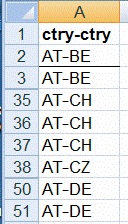
If you have a list of 11,000 rows of data in column A, which frequently changes, and you need a formula that dynamically calculates the number of unique items in the list, ignoring blanks, following are several possible solutions.
Array formulas (use Ctrl+Shift+Enter); RangeTimer indicates that this takes 13.8 seconds.
SUMPRODUCT usually calculates faster than an equivalent array formula. This formula takes 10.0 seconds, and gives an improvement factor of 13.8/10.0=1.38, which is better, but not good enough.
User-defined functions. The following code example shows a VBA user-defined function that uses the fact that the index to a collection must be unique. For an explanation of some techniques that are used, see the section about user-defined functions in the «Using functions efficiently» section in Excel performance: Tips for optimizing performance obstructions. This formula, =COUNTU(A2:A11000) , takes only 0.061 seconds. This gives an improvement factor of 13.8/0.061=226.
Adding a column of formulas. If you look at the previous sample of the data, you can see that it is sorted (Excel takes 0.5 seconds to sort the 11,000 rows). You can exploit this by adding a column of formulas that checks if the data in this row is the same as the data in the previous row. If it is different, the formula returns 1. Otherwise, it returns 0.
Add this formula to cell B2.
Copy the formula, and then add a formula to add up column B.
A full calculation of all these formulas takes 0.027 seconds. This gives an improvement factor of 13.8/0.027=511.
Conclusion
Excel enables you to effectively manage much larger worksheets, and it provides significant improvements in calculation speed compared with early versions. When you create large worksheets, it is easy to build them in a way that causes them to calculate slowly. Slow-calculating worksheets increase errors because users find it difficult to maintain concentration while calculation is occurring.
By using a straightforward set of techniques, you can speed up most slow-calculating worksheets by a factor of 10 or 100. You can also apply these techniques as you design and create worksheets to ensure that they calculate quickly.
See also
Support and feedback
Have questions or feedback about Office VBA or this documentation? Please see Office VBA support and feedback for guidance about the ways you can receive support and provide feedback.
Источник
Use Excel as your calculator
Instead of using a calculator, use Microsoft Excel to do the math!
You can enter simple formulas to add, divide, multiply, and subtract two or more numeric values. Or use the AutoSum feature to quickly total a series of values without entering them manually in a formula. After you create a formula, you can copy it into adjacent cells — no need to create the same formula over and over again.
Subtract in Excel

Multiply in Excel
Divide in Excel
Learn more about simple formulas
All formula entries begin with an equal sign (=). For simple formulas, simply type the equal sign followed by the numeric values that you want to calculate and the math operators that you want to use — the plus sign (+) to add, the minus sign (—) to subtract, the asterisk (*) to multiply, and the forward slash (/) to divide. Then, press ENTER, and Excel instantly calculates and displays the result of the formula.
For example, when you type =12.99+16.99 in cell C5 and press ENTER, Excel calculates the result and displays 29.98 in that cell.
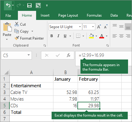
The formula that you enter in a cell remains visible in the formula bar, and you can see it whenever that cell is selected.
Important: Although there is a SUM function, there is no SUBTRACT function. Instead, use the minus (-) operator in a formula; for example, =8-3+2-4+12. Or, you can use a minus sign to convert a number to its negative value in the SUM function; for example, the formula =SUM(12,5,-3,8,-4) uses the SUM function to add 12, 5, subtract 3, add 8, and subtract 4, in that order.
Use AutoSum
The easiest way to add a SUM formula to your worksheet is to use AutoSum. Select an empty cell directly above or below the range that you want to sum, and on the Home or Formula tabs of the ribbon, click AutoSum > Sum. AutoSum will automatically sense the range to be summed and build the formula for you. This also works horizontally if you select a cell to the left or right of the range that you need to sum.
Note: AutoSum does not work on non-contiguous ranges.
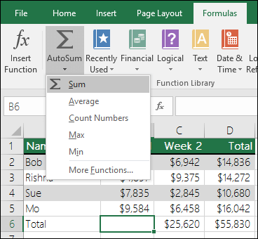
AutoSum vertically
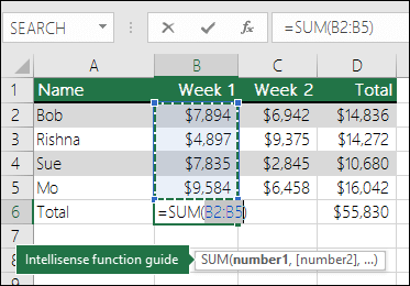
In the figure above, the AutoSum feature is seen to automatically detect cells B2:B5 as the range to sum. All you need to do is press ENTER to confirm it. If you need to add/exclude more cells, you can hold the Shift Key + the arrow key of your choice until your selection matches what you want. Then press Enter to complete the task.
Intellisense function guide: the SUM(number1,[number2], …) floating tag beneath the function is its Intellisense guide. If you click the SUM or function name, it will change o a blue hyperlink to the Help topic for that function. If you click the individual function elements, their representative pieces in the formula will be highlighted. In this case, only B2:B5 would be highlighted, since there is only one number reference in this formula. The Intellisense tag will appear for any function.
AutoSum horizontally

Learn more in the article on the SUM function.
Avoid rewriting the same formula
After you create a formula, you can copy it to other cells — no need to rewrite the same formula. You can either copy the formula, or use the fill handle  to copy the formula to adjacent cells.
For example, when you copy the formula in cell B6 to C6, the formula in that cell automatically changes to update to cell references in column C.
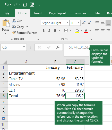
When you copy the formula, ensure that the cell references are correct. Cell references may change if they have relative references. For more information, see Copy and paste a formula to another cell or worksheet.
What can I use in a formula to mimic calculator keys?
|
Calculator key |
Excel method |
Description, example |
Result |
|
+ (Plus key) |
+ (plus) |
Use in a formula to add numbers. Example: =4+6+2 |
12 |
|
— (Minus key) |
— (minus) |
Use in a formula to subtract numbers or to signify a negative number. Example: =18-12 Example: =24*-5 (24 times negative 5) |
-120 |
|
x (Multiply key) |
* (asterisk; also called «star») |
Use in a formula to multiply numbers. Example: =8*3 |
24 |
|
÷ (Divide key) |
/ (forward slash) |
Use in a formula to divide one number by another. Example: =45/5 |
9 |
|
% (Percent key) |
% (percent) |
Use in a formula with * to multiply by a percent. Example: =15%*20 |
3 |
|
√ (square root) |
SQRT (function) |
Use the SQRT function in a formula to find the square root of a number. Example: =SQRT(64) |
8 |
|
1/x (reciprocal) |
=1/n |
Use =1/n in a formula, where n is the number you want to divide 1 by. Example: =1/8 |
0.125 |
Need more help?
You can always ask an expert in the Excel Tech Community or get support in the Answers community.
Need more help?
Want more options?
Explore subscription benefits, browse training courses, learn how to secure your device, and more.
Communities help you ask and answer questions, give feedback, and hear from experts with rich knowledge.

If you have large workbooks with a lot of formulas on the worksheets, recalculating the workbooks can take a long time. By default, Excel automatically recalculates all open workbooks as you change values in the worksheets. However, you can choose to recalculate only the current worksheet manually.
Notice I said worksheet, not workbook. There is no direct way in Excel to manually recalculate only the current workbook, but you can manually recalculate the current worksheet within a workbook.
To begin, click the “File” tab.

On the backstage screen, click “Options” in the list of items on the left.
The Excel Options dialog box displays. Click “Formulas” in the list of items on the left.
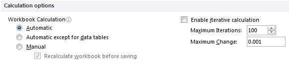
In the Calculation options section, click the “Manual” radio button to turn on the ability to manually calculate each worksheet. When you select “Manual”, the “Recalculate workbook before saving” check box is automatically checked. If you save your worksheet often and would rather not wait for it to recalculate every time you do, select the “Recalculate workbook before saving” check box so there is NO check mark in the box to disable the option.
You’ll also notice the “Automatic except for data tables” option. Data tables are defined by Microsoft as:
“. . . a range of cells that shows how changing one or two variables in your formulas will affect the results of those formulas. Data tables provide a shortcut for calculating multiple results in one operation and a way to view and compare the results of all the different variations together on your worksheet.”
Data tables are recalculated every time a worksheet is recalculated, even if they have not changed. If you’re using a lot of data tables, and you still want to automatically recalculate your workbooks, you can select the “Automatic except for data tables” option, and everything except for your data tables will be recalculated, saving you some time during recalculation.
If you don’t mind the “Recalculate workbook before saving” option being enabled when you turn on Manual calculation, there is a quicker way of choosing to manually recalculate your worksheets. First, click the “Formulas” tab.
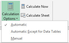
Then, in the Calculation section of the Formulas tab, click the “Calculation Options” button and select “Manual” from the drop-down menu.
Once you’ve turned on manual calculation, you can click “Calculate Sheet” in the Calculation section of the Formulas tab, or press Shift+F9, to manually recalculate the active worksheet. If you want to recalculate everything on all worksheets in all open workbooks that has changed since the last calculation, press F9 (only if you have turned off Automatic calculation). To recalculate all formulas in all open workbooks, regardless of whether they have changed since the last recalculation, press Ctrl+Alt+F9. To check formulas that depend on other cells first and then recalculate all formulas in all open workbooks, regardless of whether they have changed since the last recalculation, press Ctrl+Shift+Alt+F9.
READ NEXT
- › 12 Default Microsoft Excel Settings You Should Change
- › How to Use the Scenario Manager in Microsoft Excel
- › How to Insert Today’s Date in Microsoft Excel
- › How to Copy Values From the Status Bar in Microsoft Excel
- › How to Automatically Fill Sequential Data into Excel with the Fill Handle
- › BLUETTI Slashed Hundreds off Its Best Power Stations for Easter Sale
- › The New NVIDIA GeForce RTX 4070 Is Like an RTX 3080 for $599
- › How to Adjust and Change Discord Fonts
How-To Geek is where you turn when you want experts to explain technology. Since we launched in 2006, our articles have been read billions of times. Want to know more?
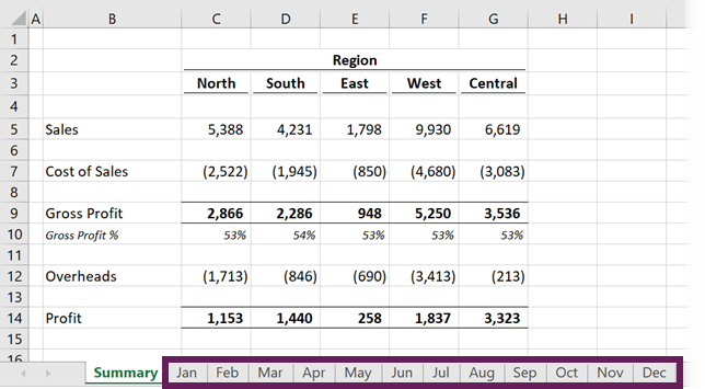
Have you ever had to sum the same cell across multiple sheets? This often occurs where information is held in numerous sheets in a consistent format. For example, it could be a monthly report with a tab for each month (see screenshot below as an example).
Watch the video
Watch the video on YouTube.
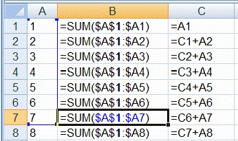
I see many examples where the user has clicked the same cell on each sheet, putting a “+” symbol between each reference. If there are a lot of worksheets, it takes a while to click on them all. Also, if the sheet names are long, the formula starts to look quite unreadable. The screenshot below shows an example of this type of approach.
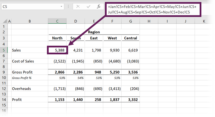
The formula in cell C5 is:
=Jan!C5+Feb!C5+Mar!C5+Apr!C5+May!C5+Jun!C5+
Jul!C5+Aug!C5+Sep!C5+Oct!C5+Nov!C5+Dec!C5
How do you know if you’ve clicked on every worksheet? What if you happened to miss one by accident? There is only one way to know – you’ve got to check it!
The chances are that you don’t need to do all that clicking. And just think about the time you will waste if there is a new tab to be added.
The good news is that there is another approach we can take that will enable us to sum across different sheets easily. I still remember the first time a work colleague showed me this trick; my jaw hit the ground in amazement. I thought he was an Excel genius. That’s why I’m sharing it here; by using this approach, you can look like an Excel genius to your work colleagues too 🙂
To sum the same cell across multiple sheets of a workbook, we can use the following formula structure:
=SUM('FirstSheet:LastSheet'!A1)
- Replace FirstSheet and LastSheet with the worksheet names you wish to sum between. If your worksheet names contain spaces, or are the name of a range (e.g., Q1 could be the name of a sheet or a cell reference ), then single quotes ( ‘ ) are required around the sheet names. If not, the single quotes can be left out.
- Replace A1 with the cell reference you wish to use
With this beautiful little formula, we can see all the worksheets included in the calculation just by looking at the tabs at the bottom. Take a look at the screenshot below. All the tabs from Jan to Dec are included in the calculation.
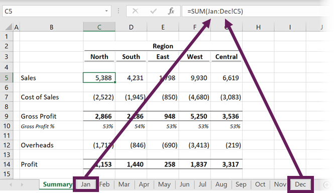
The formula in cell C5 is:
=SUM(Jan:Dec!C5)
SUM across multiple sheets – dynamic
We can change this to be more dynamic, making it even easier to use. Instead of using the names of the first and last tabs, we can create two blank sheets to act as bookends for our calculation.
Take a look at the screenshot below. The Start and End sheets are blank. By dragging sheets in and out of the Start and End bookends, we can sum almost anything we want.
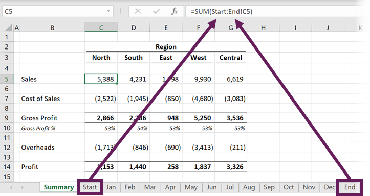
The formula in cell C5 is
=SUM(Start:End!C5)
We can also create sub-calculations. For example, we could add quarters as interim bookends too. There is the added advantage that the tabs also serve as helpful presentation dividers. The example below shows the calculation of just Jan, Feb, and Mar sheets.
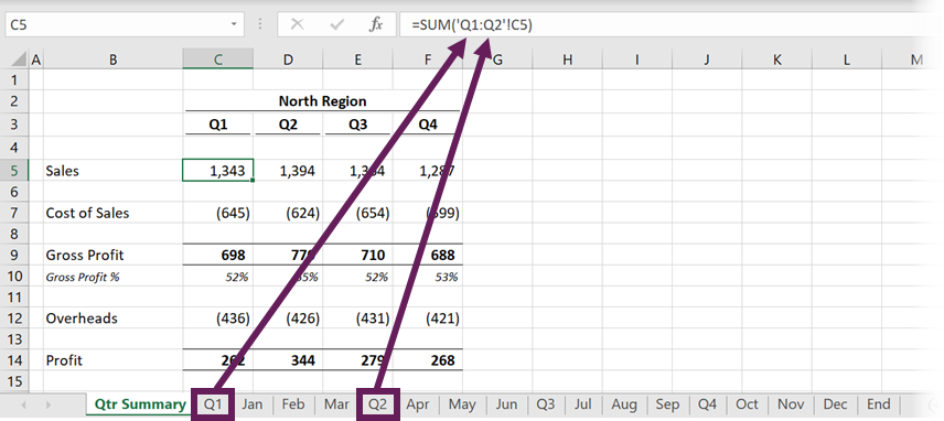
The formula in cell C5 is:
=SUM('Q1:Q2'!C5)
Excel could mistake Q1 and Q2 as cell references; therefore, adding single quotes around the sheet names is essential.
Which other formulas does this work for?
This approach doesn’t just work for the SUM function. Here is a list of all the functions for which this trick works.
| Basic Calculations
SUM AVERAGE AVERAGEA PRODUCT |
Counting
COUNT COUNTA |
Min & Max
MAX MAXA MIN MINA |
Standard deviation
STDEV STDEVA STDEVP STDEVPA |
Variance
VAR VARA VARP VARPA |
The drawbacks
There are a few things to be aware of:
- All the sheets must be in a consistent layout and must stay that way. If one worksheet changes, the formula many not sum the correct cells.
- Usually, formula cell references move automatically when new rows or columns are inserted. This formula does not work like that. It will only move if you select all the sheets and then insert a row or column into all of those sheets at the same time.
- Any sheets which are between the two tabs are included within the calculation. Therefore, even though we cannot see them, hidden sheets are also included in the result.

About the author
Hey, I’m Mark, and I run Excel Off The Grid.
My parents tell me that at the age of 7 I declared I was going to become a qualified accountant. I was either psychic or had no imagination, as that is exactly what happened. However, it wasn’t until I was 35 that my journey really began.
In 2015, I started a new job, for which I was regularly working after 10pm. As a result, I rarely saw my children during the week. So, I started searching for the secrets to automating Excel. I discovered that by building a small number of simple tools, I could combine them together in different ways to automate nearly all my regular tasks. This meant I could work less hours (and I got pay raises!). Today, I teach these techniques to other professionals in our training program so they too can spend less time at work (and more time with their children and doing the things they love).
Do you need help adapting this post to your needs?
I’m guessing the examples in this post don’t exactly match your situation. We all use Excel differently, so it’s impossible to write a post that will meet everybody’s needs. By taking the time to understand the techniques and principles in this post (and elsewhere on this site), you should be able to adapt it to your needs.
But, if you’re still struggling you should:
- Read other blogs, or watch YouTube videos on the same topic. You will benefit much more by discovering your own solutions.
- Ask the ‘Excel Ninja’ in your office. It’s amazing what things other people know.
- Ask a question in a forum like Mr Excel, or the Microsoft Answers Community. Remember, the people on these forums are generally giving their time for free. So take care to craft your question, make sure it’s clear and concise. List all the things you’ve tried, and provide screenshots, code segments and example workbooks.
- Use Excel Rescue, who are my consultancy partner. They help by providing solutions to smaller Excel problems.
What next?
Don’t go yet, there is plenty more to learn on Excel Off The Grid. Check out the latest posts:
|
Slawjan  Пользователь Сообщений: 11 |
Господа товарищи профессионалы, доброе время суток. Прикрепленные файлы
|
|
JayBhagavan  Пользователь Сообщений: 11833 ПОЛ: МУЖСКОЙ | Win10x64, MSO2019x64 |
Slawjan, опишите человеческим языком (без адресов ячеек/строк/столбцов, без формул и макросов), что Вы из чего хотите получить и по какому алгоритму? (пока я смутно понимаю суть задачи) <#0> |
|
Slawjan Пользователь Сообщений: 11 |
JayBhagavan, |
|
JayBhagavan Пользователь Сообщений: 11833 ПОЛ: МУЖСКОЙ | Win10x64, MSO2019x64 |
#4 28.10.2018 07:06:54
Опять 25.
форума. (до исправления названия модераторами, помощь не рекомендуется оказывать, т.е. предоставлять решение макросами и/или формулами) Изменено: JayBhagavan — 28.10.2018 07:07:44 <#0> |
||||
|
Slawjan Пользователь Сообщений: 11 |
Попробую конкретнее: Изменено: Slawjan — 28.10.2018 07:31:53 |
|
JayBhagavan Пользователь Сообщений: 11833 ПОЛ: МУЖСКОЙ | Win10x64, MSO2019x64 |
#6 28.10.2018 07:30:36
<#0> |
||
|
Slawjan Пользователь Сообщений: 11 |
#7 28.10.2018 07:34:22
Мне нужен подсчёт количества «считываний» iD каждого прибора (при выдаче, при сдаче прибора). |
||
|
gling  Пользователь Сообщений: 4024 |
#8 28.10.2018 07:46:04 Здравствуйте. Может эта формула в столбец F подойдёт?
|
||
|
Slawjan Пользователь Сообщений: 11 |
Добрый день. Спасибо, но к сожалению нет. Идеальная формула была бы F1=F1+E1, но такого не бывает))) Плюс формулы работают только «онлайн» и не сохраняют данные. Макрос позволяет «вбить» в ячейку данные, которые там и останутся при закрытии/открытии файла….. |
|
Slawjan Пользователь Сообщений: 11 |
#10 28.10.2018 08:17:19 Ладно, по-другому:
|
||
|
bedvit  Пользователь Сообщений: 2477 Виталий |
#11 28.10.2018 08:51:27
бывает, примеров куча, первый попавшийся . Только нужно понимать для чего это делается и как это работает. Изменено: bedvit — 28.10.2018 08:51:56 «Бритва Оккама» или «Принцип Калашникова»? |
||
|
Slawjan Пользователь Сообщений: 11 |
#12 28.10.2018 09:01:13 Последний более-менее рабочий макрос, что смог «наваять»:
Но проблема в том, что он обрабатывает не только ту ячейку, которая была изменена последней, а и остальные……. |
||
|
БМВ  Модератор Сообщений: 21376 Excel 2013, 2016 |
#13 28.10.2018 09:08:13
не надо туда По вопросам из тем форума, личку не читаю. |
||

|
gling Пользователь Сообщений: 4024 |
#14 28.10.2018 09:15:50 По вашему описанию, если код прописан на Sheet2, макрос можно записать так
Но у вас либо ошибка, либо вы задумали для меня не понятное. Формула в Sheet1 «E1″=Sheet2 «Z3» не учитывая ID в столбце А, почему? Получается что в столбце Е Sheet1, счет не связан с данными на листе Sheet1, все данные берутся с другого листа. Это и не понятно.
Изменено: gling — 28.10.2018 09:26:31 |
||||
|
Slawjan Пользователь Сообщений: 11 |
Прошу прощения, в файле много лишнего было. Не поудалял полностью все «попытки». Во вложении «подчищенный» файл. Прикрепленные файлы
Изменено: Slawjan — 28.10.2018 09:51:11 |
|
Slawjan Пользователь Сообщений: 11 |
#16 28.10.2018 10:06:46
А Worksheet.Calculate же не работает с Target? А если Worksheet.Change использовать, то он не работает с ячейками, содержащими формулы…. |
||
|
БМВ Модератор Сообщений: 21376 Excel 2013, 2016 |
Slawjan, #13 вы читали или нет? По вопросам из тем форума, личку не читаю. |
|
Slawjan Пользователь Сообщений: 11 |
БМВ, читал)))) Пытаюсь сформулировать теперь и порпобовать |
|
gling Пользователь Сообщений: 4024 |
Вариант в файле, но не понятно может ли быть два одинаковых ID на листе 2? Если да то что то будет не так, потому что формула в столбце Е учитывает только наличие ID на листе2 Прикрепленные файлы
Изменено: gling — 28.10.2018 10:53:05 |
|
Slawjan Пользователь Сообщений: 11 |
#20 28.10.2018 11:16:12
Ну, блин, всё гениальное оказывается просто))))) А я прилип к этому «ЕСЛИ» в Sheet1 «D» и всё больше на этом зацикливался…. А то, что можно же по другой позиции найти и потом счёт к этому привязать…. |
||
|
vikttur Пользователь Сообщений: 47199 |
#21 29.10.2018 13:31:37 А теперь модераторы ждут от провинившихся название темы. Предложение автора:
Но это что-то закрученное и непонятное. |
||
Return to VBA Code Examples
In this Article
- Calculate Now
- Calculate Sheet Only
- Calculate Range
- Calculate Individual Formula
- Calculate Workbook
- Calculate Workbook – Methods That Don’t Work
This tutorial will teach you all of the different Calculate options in VBA.
By default Excel calculates all open workbooks every time a workbook change is made. It does this by following a calculation tree where if cell A1 is changed, it updates all cells that rely on cell A1 and so on. However, this can cause your VBA code to run extremely slowly, as every time a cell changes, Excel must re-calculate.
To increase your VBA speed, you will often want to disable automatic calculations at the beginning of your procedures:
Application.Calculation = xlManualand re-enable it at the end:
Application.Calculation = xlAutomaticHowever, what if you want to calculate all (or part) of your workbooks within your procedure? The rest of this tutorial will teach you what to do.
Calculate Now
You can use the Calculate command to re-calculate everything (in all open workbooks):
CalculateThis is usually the best method to use. However, you can also perform more narrow calculations for improved speed.
Calculate Sheet Only
You can also tell VBA to calculate only a specific sheet.
This code will recalculate the active sheet:
ActiveSheet.CalculateThis code will recalculate Sheet1:
Sheets("Sheet1").CalculateCalculate Range
If you require a more narrow calculation, you can tell VBA to calculate only a range of cells:
Sheets("Sheet1").Range("a1:a10").CalculateCalculate Individual Formula
This code will calculate only an individual cell formula:
Range("a1").CalculateCalculate Workbook
There is no VBA option to calculate only an entire workbook. If you need to calculate an entire workbook, the best option is to use the Calculate command:
CalculateThis will calculate all open workbooks. If you’re really concerned about speed, and want to calculate an entire workbook, you might be able to be more selective about which workbooks are open at one time.
Calculate Workbook – Methods That Don’t Work
There are a couple of methods that you might be tempted to use to force VBA to calculate just a workbook, however none of them will work properly.
This code will loop through each worksheet in the workbook and recalculate the sheets one at a time:
Sub Recalculate_Workbook()
    Dim ws As Worksheet

    For Each ws In Worksheets
        ws.Calculate
    Next ws
End Sub
This code will work fine if all of your worksheets are “self-contained”, meaning none of your sheets contain calculations that refer to other sheets.
However, if your worksheets refer to other sheets, your calculations might not update properly. For example, if you calculate Sheet1 before Sheet2, but Sheet1’s formulas rely on calculations done in Sheet2 then your formulas will not contain the most up-to-date values.
You might also try selecting all sheets at once and calculating the activesheet:
ThisWorkbook.Sheets.Select
ActiveSheet.Calculate
However, this will cause the same issue.
VBA Coding Made Easy
Stop searching for VBA code online. Learn more about AutoMacro — A VBA Code Builder that allows beginners to code procedures from scratch with minimal coding knowledge and with many time-saving features for all users!

Learn More!