
Excel for Microsoft 365 Excel for Microsoft 365 for Mac Excel for the web Excel 2021 Excel 2021 for Mac Excel 2019 Excel 2019 for Mac Excel 2016 Excel 2016 for Mac Excel 2013 More…Less
If you need a quick way to count rows that contain data, select all the cells in the first column of that data (it may not be column A). Just click the column header. The status bar, in the lower-right corner of your Excel window, will tell you the row count.
Do the same thing to count columns, but this time click the row selector at the left end of the row.
The status bar then displays a count, something like this:

If you select an entire row or column, Excel counts just the cells that contain data. If you select a block of cells, it counts the number of cells you selected. If the row or column you select contains only one cell with data, the status bar stays blank.
Notes:
-
If you need to count the characters in cells, see Count characters in cells.
-
If you want to know how many cells have data, see Use COUNTA to count cells that aren’t blank.
-
You can control the messages that appear in the status bar by right-clicking the status bar and clicking the item you want to see or remove. For more information, see Excel status bar options.
Need more help?
You can always ask an expert in the Excel Tech Community or get support in the Answers community.
Need more help?
If you need to sum a column or row of numbers, let Excel do the math for you. Select a cell next to the numbers you want to sum, click AutoSum on the Home tab, press Enter, and you’re done. When you click AutoSum, Excel automatically enters a formula (that uses the SUM function) to sum the numbers. Here’s an example.
Contents
- 1 How do I calculate multiple rows in Excel?
- 2 How do I calculate 3 rows in Excel?
- 3 How do I apply a formula to multiple rows?
- 4 What does row 1 1 do in Excel?
- 5 What does row () mean in Excel?
- 6 What does () mean in Excel?
- 7 How do I apply a formula to an entire column in Excel?
- 8 How will you select an entire row in a table?
- 9 How do I sum multiple rows in Excel based on criteria?
- 10 How do you use a row formula?
- 11 What is an Xlookup in Excel?
- 12 Why am I getting ### in Excel?
- 13 Where is the formula on Excel?
- 14 What does a $1 mean in Excel?
- 15 How do you apply formula to entire column in Excel without dragging?
- 16 How do you apply a formula to a column in sheets?
- 17 How do I select a row in Excel?
- 18 How do I select all rows in Excel with data?
- 19 How do I quickly select thousands of rows in Excel?
How do I calculate multiple rows in Excel?
Hold Ctrl + Shift key together; first press the left arrow to select the complete row then, by holding Ctrl + Shift key together, press Down Arrow to select the complete column. Like this, we can select multiple rows in excel without much trouble.
Excel ROWS Function
- Summary. The Excel ROWS function returns the count of rows in a given reference. For example, ROWS(A1:A3) returns 3, since the range A1:A3 contains 3 rows.
- Get the number of rows in an array or reference.
- Number of rows.
- =ROWS (array)
- array – A reference to a cell or range of cells.
How do I apply a formula to multiple rows?
Simply do the following:
- Select the cell with the formula and the adjacent cells you want to fill.
- Click Home > Fill, and choose either Down, Right, Up, or Left. Keyboard shortcut: You can also press Ctrl+D to fill the formula down in a column, or Ctrl+R to fill the formula to the right in a row.
What does row 1 1 do in Excel?
Excel row function examples, with Rows, Row(A:A), Row(1:1) and add even or odd rows. The Row function is used to return the row number of a reference cell or a range of cells in Excel. If the argument is omitted, it will return the row number of the row in which the formula is located.
What does row () mean in Excel?
The Microsoft Excel ROW function returns the row number of a cell reference. The ROW function is a built-in function in Excel that is categorized as a Lookup/Reference Function. It can be used as a worksheet function (WS) in Excel.
What does () mean in Excel?
() Parentheses. All Arguments of the Excel Functions specified between the Parentheses. Example:=COUNTIF(A1:A5,5) ()
How do I apply a formula to an entire column in Excel?
The easiest way to apply a formula to the entire column in all adjacent cells is by double-clicking the fill handle by selecting the formula cell. In this example, we need to select the cell F2 and double click on the bottom right corner. Excel applies the same formula to all the adjacent cells in the entire column F.
How will you select an entire row in a table?
Click the left border of the table row. The following selection arrow appears to indicate that clicking selects the row. You can click the first cell in the table row, and then press CTRL+SHIFT+RIGHT ARROW.
How do I sum multiple rows in Excel based on criteria?
Sum multiple columns based on single criteria with an awesome feature
- Select Lookup and sum matched value(s) in row(s) option under the Lookup and Sum Type section;
- Specify the lookup value, output range and the data range that you want to use;
- Select Return the sum of all matched values option from the Options.
How do you use a row formula?
The ROW function returns the row number for a cell or range. For example, =ROW(C3) returns 3, since C3 is the third row in the spreadsheet. When no reference is provided, ROW returns the row number of the cell which contains the formula.
What is an Xlookup in Excel?
Use the XLOOKUP function to find things in a table or range by row.With XLOOKUP, you can look in one column for a search term, and return a result from the same row in another column, regardless of which side the return column is on.
Why am I getting ### in Excel?
Microsoft Excel might show ##### in cells when a column isn’t wide enough to show all of the cell contents. Formulas that return dates and times as negative values can also show as #####.If dates are too long, click Home > arrow next to Number Format, and pick Short Date.
Where is the formula on Excel?
See a formula
When a formula is entered into a cell, it also appears in the Formula bar. To see a formula, select a cell, and it will appear in the formula bar.
What does a $1 mean in Excel?
A$1. Allows the column reference to change, but not the row reference. $A$1. Allows neither the column nor the row reference to change. There is a shortcut for placing absolute cell references in your formulas!
How do you apply formula to entire column in Excel without dragging?
7 Answers
- First put your formula in F1.
- Now hit ctrl+C to copy your formula.
- Hit left, so E1 is selected.
- Now hit Ctrl+Down.
- Now hit right so F20000 is selected.
- Now hit ctrl+shift+up.
- Finally either hit ctrl+V or just hit enter to fill the cells.
How do you apply a formula to a column in sheets?
How To Use Formulas In Google Sheets
- Double click on the cell where you want your formula, and then type “=” without quotes, followed by the formula.
- Press Enter to save formula or click on another cell. The results will appear in the cell while the formula will show in the “fx” box above.
How do I select a row in Excel?
Select one or more rows and columns
Or click on any cell in the column and then press Ctrl + Space. Select the row number to select the entire row. Or click on any cell in the row and then press Shift + Space. To select non-adjacent rows or columns, hold Ctrl and select the row or column numbers.
How do I select all rows in Excel with data?
Select Entire Rows in a Worksheet
- Click on a worksheet cell in the row to be selected to make it the active cell.
- Press and hold the Shift key on the keyboard.
- Press and release the Spacebar key on the keyboard.
- Release the Shift key.
- All cells in the selected row are highlighted; including the row header.
How do I quickly select thousands of rows in Excel?
Select Multiple Entire Rows of Cells.
Continuing to hold down your mouse button, drag your cursor across all the rows you want to select. Or, if you prefer, you can hold down your Shift key and click the bottom-most row you want to select.
How to Count the Number of Rows in Excel?
Here are the different ways of counting rows in Excel using the formula, rows with data, empty rows, rows with numerical values, rows with text values, and many other things related to counting the number of rows in Excel.
You can download this Count Rows Excel Template here – Count Rows Excel Template
Table of contents
- How to Count the Number of Rows in Excel?
- #1 – Excel Count Rows which has only the Data
- #2 – Count all the rows that have the data
- #3 – Count the rows that only have the numbers
- #4 – Count Rows, which only has the Blanks
- #5 – Count rows that only have text values
- #6 – Count all of the rows in the range
- Things to Remember
- Recommended Articles
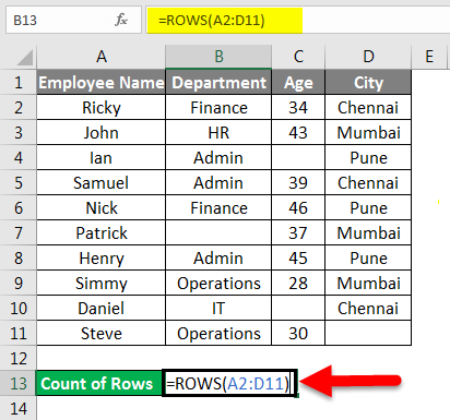
#1 – Excel Count Rows which has only the Data
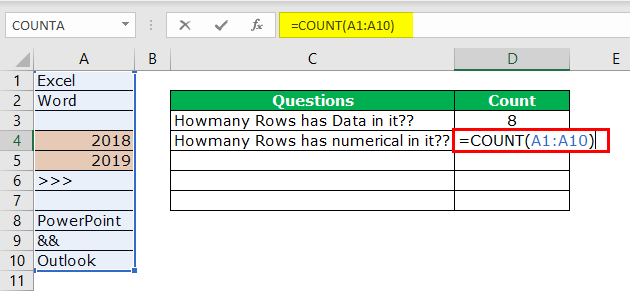
Firstly, we will see how to count the number of rows in Excel with the data. There could be empty rows between the data, but we often need to ignore them and find exactly how many rows contain the data in it.
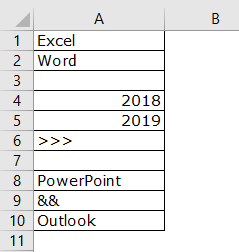
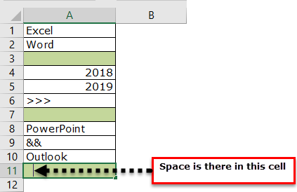
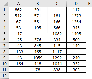
- We can count the number of rows with data by selecting the range of cells in Excel. For example, take a look at the below data.

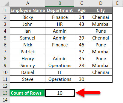
We have a total of 10 rows (border inserted area). In this 10 row, we want to count exactly how many cells have data. Since this is a small list of rows, we can easily calculate the number of rows. But when it comes to the huge database, it is impossible to count manually. So, this article will help you with this.
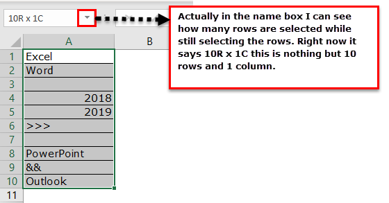
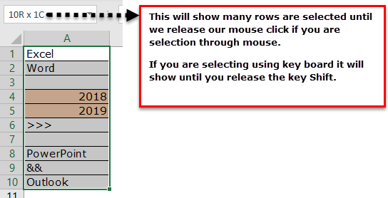
- Firstly, we must select all the rows in Excel.

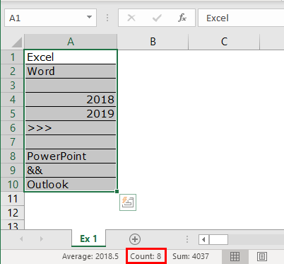
- It is not telling us how many rows contain the data here. Instead, look at the Excel screen’s right-hand side bottom, i.e., a status bar.

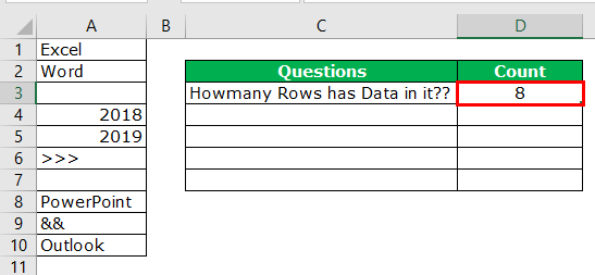
Take a look at the red circled area. It says COUNT as 8, which means that out of 10 selected rows, 8 have data.
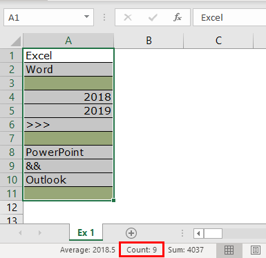
- Now, we will select one more row in the range and see what the count will be.

- We have selected 11 rows, but the count says 9, whereas we have data only in 8 rows. When we closely examine the cells, the 11th row contains a space.

Even though there is no value in the cell and it has only space Excel will be treated as the cell which contains the data.
#2 – Count all the rows that have the data
We know how to check how many rows contain the data quickly. But that is not the dynamic way of counting rows that have data. Instead, we need to apply the COUNTA function to count how many rows contain the data.
We will apply the COUNTA function in the D3 cell.
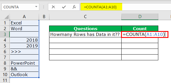
So, the total number of rows containing the data is 8 rows. Even this formula treats space as data.
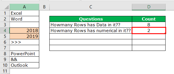
#3 – Count the rows that only have the numbers
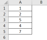
Here we want to count how many rows contain only numerical values.
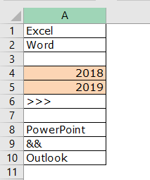
We can easily say 2 rows contain numerical values. Let us examine this by using a formula. We have a built-in formula called COUNT which counts only numerical values in the supplied range.
![]()
We will apply the COUNT function in cell B1 and select the range as A1 to A10.
The COUNT function also says 2 as a result. So, out of 10 rows, only rows contain numerical values.
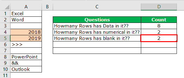
#4 – Count Rows, which only has the Blanks
We can find only blank rows by using the COUNTBLANK function in Excel.
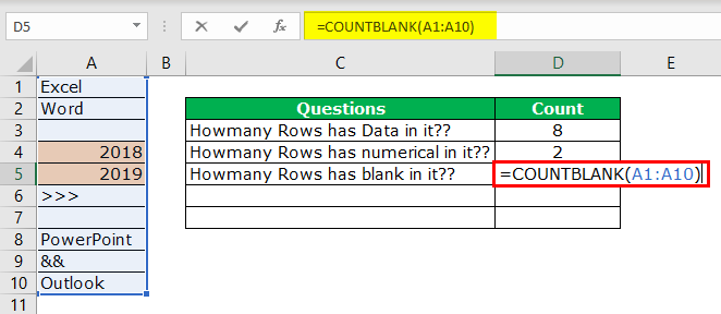
We have 2 blank rows in the selected range, which are revealed by the count blank function.
#5 – Count rows that only have text values
Remember, we do not have any straight in the COUNTTEXT function. Unlike in previous cases, we need to think differently here. We can use the COUNTIF functionThe COUNTIF function in Excel counts the number of cells within a range based on pre-defined criteria. It is used to count cells that include dates, numbers, or text. For example, COUNTIF(A1:A10,”Trump”) will count the number of cells within the range A1:A10 that contain the text “Trump”
read more with a wildcard character asterisk (*).
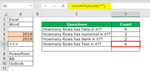
Here all the magic is done by the wildcard character asterisk (*). It matches any of the alphabets in the row and returns the result as a text value row. Even if the row contains numerical and text values, it will be treated as text value only.
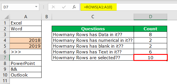
#6 – Count all of the rows in the range
Now comes the important part. How do we count how many rows we have selected? One uses the Name Box in excel, which is limited while still choosing the rows. But how do we measure then?
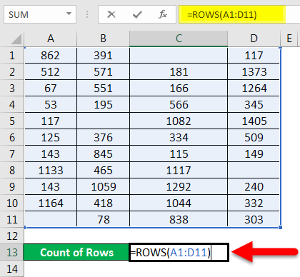
We have a built-in ROWS formula, which returns how many rows are selected.
Things to Remember
- Even space is treated as a value in the cell.
- If the cell contains numerical and text values, it will be treated as a text value.
- ROW may return the current row we are in, but ROWS will return how many are in the supplied range even though there is no data in the rows.
Recommended Articles
This article has been a guide to Count Rows in Excel. Here, we discuss the top 6 ways of counting rows in Excel using the formula: rows with data, empty rows, rows with numerical values, rows with text values, and many other things related to counting rows in Excel and practical examples and downloadable Excel templates. You may learn more about Excel from the following articles: –
- VBA COUNTIF
- Add Multiple Rows in Excel
- Excel Count Formula
- How to Insert Multiple Rows in Excel?
Содержание
- Ways to count values in a worksheet
- Download our examples
- In this article
- Simple counting
- Video: Count cells by using the Excel status bar
- Use AutoSum
- Add a Subtotal row
- Count cells in a list or Excel table column by using the SUBTOTAL function
- Counting based on one or more conditions
- Video: Use the COUNT, COUNTIF, and COUNTA functions
- Count cells in a range by using the COUNT function
- Count cells in a range based on a single condition by using the COUNTIF function
- Count cells in a column based on single or multiple conditions by using the DCOUNT function
- Count cells in a range based on multiple conditions by using the COUNTIFS function
- Count based on criteria by using the COUNT and IF functions together
- Count how often multiple text or number values occur by using the SUM and IF functions together
- Count cells in a column or row in a PivotTable
- Counting when your data contains blank values
- Count nonblank cells in a range by using the COUNTA function
- Count nonblank cells in a list with specific conditions by using the DCOUNTA function
- Count blank cells in a contiguous range by using the COUNTBLANK function
- Count blank cells in a non-contiguous range by using a combination of SUM and IF functions
- Counting unique occurrences of values
- Count the number of unique values in a list column by using Advanced Filter
- Count the number of unique values in a range that meet one or more conditions by using IF, SUM, FREQUENCY, MATCH, and LEN functions
- Special cases (count all cells, count words)
- Count the total number of cells in a range by using ROWS and COLUMNS functions
- Count words in a range by using a combination of SUM, IF, LEN, TRIM, and SUBSTITUTE functions
- Displaying calculations and counts on the status bar
- Need more help?
Ways to count values in a worksheet
Counting is an integral part of data analysis, whether you are tallying the head count of a department in your organization or the number of units that were sold quarter-by-quarter. Excel provides multiple techniques that you can use to count cells, rows, or columns of data. To help you make the best choice, this article provides a comprehensive summary of methods, a downloadable workbook with interactive examples, and links to related topics for further understanding.
Note: Counting should not be confused with summing. For more information about summing values in cells, columns, or rows, see Summing up ways to add and count Excel data.
Download our examples
You can download an example workbook that gives examples to supplement the information in this article. Most sections in this article will refer to the appropriate worksheet within the example workbook that provides examples and more information.
In this article
Simple counting
You can count the number of values in a range or table by using a simple formula, clicking a button, or by using a worksheet function.
Excel can also display the count of the number of selected cells on the Excel status bar. See the video demo that follows for a quick look at using the status bar. Also, see the section Displaying calculations and counts on the status bar for more information. You can refer to the values shown on the status bar when you want a quick glance at your data and don’t have time to enter formulas.
Video: Count cells by using the Excel status bar
Watch the following video to learn how to view count on the status bar.

Use AutoSum
Use AutoSum by selecting a range of cells that contains at least one numeric value. Then on the Formulas tab, click AutoSum > Count Numbers.

Excel returns the count of the numeric values in the range in a cell adjacent to the range you selected. Generally, this result is displayed in a cell to the right for a horizontal range or in a cell below for a vertical range.
Add a Subtotal row
You can add a subtotal row to your Excel data. Click anywhere inside your data, and then click Data > Subtotal.
Note: The Subtotal option will only work on normal Excel data, and not Excel tables, PivotTables, or PivotCharts.

Also, refer to the following articles:
Count cells in a list or Excel table column by using the SUBTOTAL function
Use the SUBTOTAL function to count the number of values in an Excel table or range of cells. If the table or range contains hidden cells, you can use SUBTOTAL to include or exclude those hidden cells, and this is the biggest difference between SUM and SUBTOTAL functions.
The SUBTOTAL syntax goes like this:

To include hidden values in your range, you should set the function_num argument to 2.
To exclude hidden values in your range, set the function_num argument to 102.
Counting based on one or more conditions
You can count the number of cells in a range that meet conditions (also known as criteria) that you specify by using a number of worksheet functions.
Video: Use the COUNT, COUNTIF, and COUNTA functions
Watch the following video to see how to use the COUNT function and how to use the COUNTIF and COUNTA functions to count only the cells that meet conditions you specify.
Count cells in a range by using the COUNT function
Use the COUNT function in a formula to count the number of numeric values in a range.

In the above example, A2, A3, and A6 are the only cells that contains numeric values in the range, hence the output is 3.
Note: A7 is a time value, but it contains text ( a.m.), hence COUNT does not consider it a numerical value. If you were to remove a.m. from the cell, COUNT will consider A7 as a numerical value, and change the output to 4.
Count cells in a range based on a single condition by using the COUNTIF function
Use the COUNTIF function function to count how many times a particular value appears in a range of cells.

Count cells in a column based on single or multiple conditions by using the DCOUNT function
DCOUNT function counts the cells that contain numbers in a field (column) of records in a list or database that match conditions that you specify.
In the following example, you want to find the count of the months including or later than March 2016 that had more than 400 units sold. The first table in the worksheet, from A1 to B7, contains the sales data.

DCOUNT uses conditions to determine where the values should be returned from. Conditions are typically entered in cells in the worksheet itself, and you then refer to these cells in the criteria argument. In this example, cells A10 and B10 contain two conditions—one that specifies that the return value must be greater than 400, and the other that specifies that the ending month should be equal to or greater than March 31st, 2016.
You should use the following syntax:
DCOUNT checks the data in the range A1 through B7, applies the conditions specified in A10 and B10, and returns 2, the total number of rows that satisfy both conditions (rows 5 and 7).
Count cells in a range based on multiple conditions by using the COUNTIFS function
The COUNTIFS function is similar to the COUNTIF function with one important exception: COUNTIFS lets you apply criteria to cells across multiple ranges and counts the number of times all criteria are met. You can use up to 127 range/criteria pairs with COUNTIFS.
The syntax for COUNTIFS is:
COUNTIFS(criteria_range1, criteria1, [criteria_range2, criteria2],…)
See the following example:

Count based on criteria by using the COUNT and IF functions together
Let’s say you need to determine how many salespeople sold a particular item in a certain region or you want to know how many sales over a certain value were made by a particular salesperson. You can use the IF and COUNT functions together; that is, you first use the IF function to test a condition and then, only if the result of the IF function is True, you use the COUNT function to count cells.
The formulas in this example must be entered as array formulas. If you have opened this workbook in Excel for Windows or Excel 2016 for Mac and want to change the formula or create a similar formula, press F2, and then press Ctrl+Shift+Enter to make the formula return the results you expect. In earlier versions of Excel for Mac, use  +Shift+Enter.
For the example formulas to work, the second argument for the IF function must be a number.

Count how often multiple text or number values occur by using the SUM and IF functions together
In the examples that follow, we use the IF and SUM functions together. The IF function first tests the values in some cells and then, if the result of the test is True, SUM totals those values that pass the test.

The above function says if C2:C7 contains the values Buchanan and Dodsworth, then the SUM function should display the sum of records where the condition is met. The formula finds three records for Buchanan and one for Dodsworth in the given range, and displays 4.

The above function says if D2:D7 contains values lesser than $9000 or greater than $19,000, then SUM should display the sum of all those records where the condition is met. The formula finds two records D3 and D5 with values lesser than $9000, and then D4 and D6 with values greater than $19,000, and displays 4.

The above function says if D2:D7 has invoices for Buchanan for less than $9000, then SUM should display the sum of records where the condition is met. The formula finds that C6 meets the condition, and displays 1.
Important: The formulas in this example must be entered as array formulas. That means you press F2 and then press Ctrl+Shift+Enter. In earlier versions of Excel for Mac use +Shift+Enter.
See the following Knowledge Base articles for additional tips:
Count cells in a column or row in a PivotTable
A PivotTable summarizes your data and helps you analyze and drill down into your data by letting you choose the categories on which you want to view your data.
You can quickly create a PivotTable by selecting a cell in a range of data or Excel table and then, on the Insert tab, in the Tables group, clicking PivotTable.

Let’s look at a sample scenario of a Sales spreadsheet, where you can count how many sales values are there for Golf and Tennis for specific quarters.
Note: For an interactive experience, you can run these steps on the sample data provided in the PivotTable sheet in the downloadable workbook.
Enter the following data in an Excel spreadsheet.

Click Insert > PivotTable.
In the Create PivotTable dialog box, click Select a table or range, then click New Worksheet, and then click OK.
An empty PivotTable is created in a new sheet.
In the PivotTable Fields pane, do the following:
Drag Sport to the Rows area.
Drag Quarter to the Columns area.
Drag Sales to the Values area.
The field name displays as SumofSales2 in both the PivotTable and the Values area.
At this point, the PivotTable Fields pane looks like this:

In the Values area, click the dropdown next to SumofSales2 and select Value Field Settings.
In the Value Field Settings dialog box, do the following:
In the Summarize value field by section, select Count.
In the Custom Name field, modify the name to Count.

The PivotTable displays the count of records for Golf and Tennis in Quarter 3 and Quarter 4, along with the sales figures.

Counting when your data contains blank values
You can count cells that either contain data or are blank by using worksheet functions.
Count nonblank cells in a range by using the COUNTA function
Use the COUNTA function function to count only cells in a range that contain values.
When you count cells, sometimes you want to ignore any blank cells because only cells with values are meaningful to you. For example, you want to count the total number of salespeople who made a sale (column D).

COUNTA ignores the blank values in D3, D4, D8, and D11, and counts only the cells containing values in column D. The function finds six cells in column D containing values and displays 6 as the output.
Count nonblank cells in a list with specific conditions by using the DCOUNTA function
Use the DCOUNTA function to count nonblank cells in a column of records in a list or database that match conditions that you specify.
The following example uses the DCOUNTA function to count the number of records in the database that is contained in the range A1:B7 that meet the conditions specified in the criteria range A9:B10. Those conditions are that the Product ID value must be greater than or equal to 2000 and the Ratings value must be greater than or equal to 50.

DCOUNTA finds two rows that meet the conditions- rows 2 and 4, and displays the value 2 as the output.
Count blank cells in a contiguous range by using the COUNTBLANK function
Use the COUNTBLANK function function to return the number of blank cells in a contiguous range (cells are contiguous if they are all connected in an unbroken sequence). If a cell contains a formula that returns empty text («»), that cell is counted.
When you count cells, there may be times when you want to include blank cells because they are meaningful to you. In the following example of a grocery sales spreadsheet. suppose you want to find out how many cells don’t have the sales figures mentioned.

Note: The COUNTBLANK worksheet function provides the most convenient method for determining the number of blank cells in a range, but it doesn’t work very well when the cells of interest are in a closed workbook or when they do not form a contiguous range. The Knowledge Base article XL: When to Use SUM(IF()) instead of CountBlank() shows you how to use a SUM(IF()) array formula in those cases.
Count blank cells in a non-contiguous range by using a combination of SUM and IF functions
Use a combination of the SUM function and the IF function. In general, you do this by using the IF function in an array formula to determine whether each referenced cell contains a value, and then summing the number of FALSE values returned by the formula.
See a few examples of SUM and IF function combinations in an earlier section Count how often multiple text or number values occur by using the SUM and IF functions together in this topic.
Counting unique occurrences of values
You can count unique values in a range by using a PivotTable, COUNTIF function, SUM and IF functions together, or the Advanced Filter dialog box.
Count the number of unique values in a list column by using Advanced Filter
Use the Advanced Filter dialog box to find the unique values in a column of data. You can either filter the values in place or you can extract and paste them to a new location. Then you can use the ROWS function to count the number of items in the new range.
To use Advanced Filter, click the Data tab, and in the Sort & Filter group, click Advanced.
The following figure shows how you use the Advanced Filter to copy only the unique records to a new location on the worksheet.

In the following figure, column E contains the values that were copied from the range in column D.

If you filter your data in place, values are not deleted from your worksheet — one or more rows might be hidden. Click Clear in the Sort & Filter group on the Data tab to display those values again.
If you only want to see the number of unique values at a quick glance, select the data after you have used the Advanced Filter (either the filtered or the copied data) and then look at the status bar. The Count value on the status bar should equal the number of unique values.
Count the number of unique values in a range that meet one or more conditions by using IF, SUM, FREQUENCY, MATCH, and LEN functions
Use various combinations of the IF, SUM, FREQUENCY, MATCH, and LEN functions.
For more information and examples, see the section «Count the number of unique values by using functions» in the article Count unique values among duplicates.
Special cases (count all cells, count words)
You can count the number of cells or the number of words in a range by using various combinations of worksheet functions.
Count the total number of cells in a range by using ROWS and COLUMNS functions
Suppose you want to determine the size of a large worksheet to decide whether to use manual or automatic calculation in your workbook. To count all the cells in a range, use a formula that multiplies the return values using the ROWS and COLUMNS functions. See the following image for an example:

Count words in a range by using a combination of SUM, IF, LEN, TRIM, and SUBSTITUTE functions
You can use a combination of the SUM, IF, LEN, TRIM, and SUBSTITUTE functions in an array formula. The following example shows the result of using a nested formula to find the number of words in a range of 7 cells (3 of which are empty). Some of the cells contain leading or trailing spaces — the TRIM and SUBSTITUTE functions remove these extra spaces before any counting occurs. See the following example:

Now, for the above formula to work correctly, you have to make this an array formula, otherwise the formula returns the #VALUE! error. To do that, click on the cell that has the formula, and then in the Formula bar, press Ctrl + Shift + Enter. Excel adds a curly bracket at the beginning and the end of the formula, thus making it an array formula.
For more information on array formulas, see Overview of formulas in Excel and Create an array formula.
Displaying calculations and counts on the status bar
When one or more cells are selected, information about the data in those cells is displayed on the Excel status bar. For example, if four cells on your worksheet are selected, and they contain the values 2, 3, a text string (such as «cloud»), and 4, all of the following values can be displayed on the status bar at the same time: Average, Count, Numerical Count, Min, Max, and Sum. Right-click the status bar to show or hide any or all of these values. These values are shown in the illustration that follows.

Need more help?
You can always ask an expert in the Excel Tech Community or get support in the Answers community.
Источник

Excel Row Count (Table of Contents)
- Introduction to Row Count in Excel
- How to Count the Rows in Excel?
Introduction to Row Count in Excel
Excel provides many built-in functions through which we can do multiple calculations. We can also count the rows and columns in Excel. Here in this article, we will discuss the Row Count in Excel. If we want to measure the rows which contain data, select all the cells of the first column by clicking on the column header. It will display the row count on the status bar in the lower right corner.
Let’s take some values in the Excel sheet.
Select the entire column which contains data. Now click on the column label for counting the rows; it will show you the row count. Refer to the below screenshot:

There are two types of functions for counting the rows.
- ROW()
- ROWS()
The ROW() function gives you the row number of a particular cell.
The ROWS() function gives you the count of rows in a range.
How to Count the Rows in Excel?
Let’s take some examples to understand the usage of ROWS functions.
You can download this Row Count Excel Template here – Row Count Excel Template
Example #1
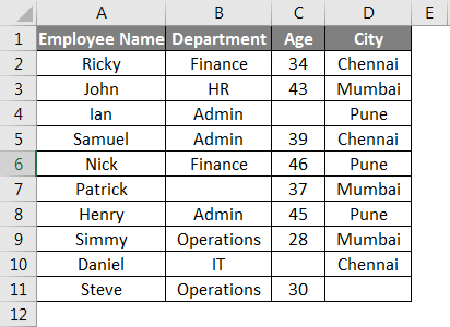
We have given the below employee data.
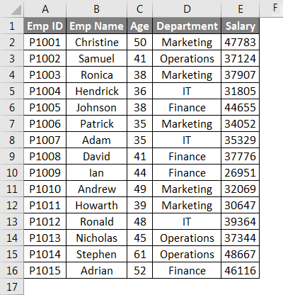
For counting the rows here, we will use the below function here:
=ROWS(range)
Where range = a range of cells containing data.
Now we will apply the above function like the below screenshot:

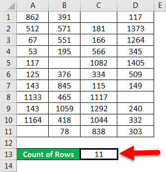
Which returns the number of rows containing the data in the supplied range.
The final result is given below:
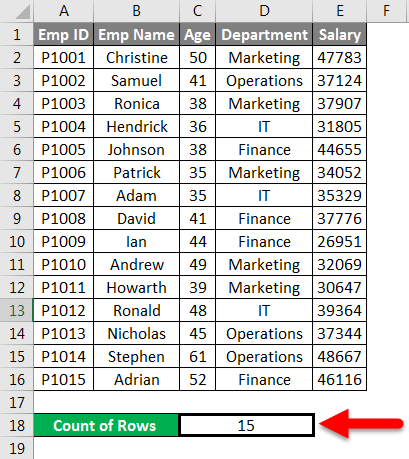
Example #2
We have given below some student marks subject-wise.
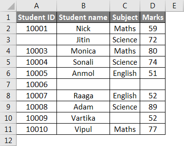
As we can see in the above dataset, certain information is absent.
As per the screenshot below, we will apply the ROWS function for counting the rows containing data.
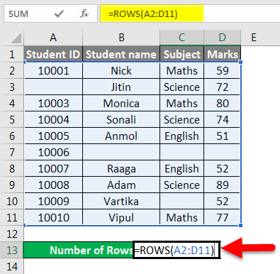
The final result is given below:

Example #3
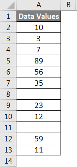
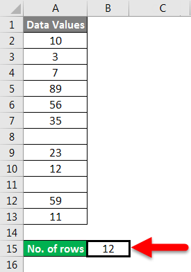
We have given the below data values.
We will pass the range of data values within the function for counting the number of rows.
Apply the function like the below screenshot:
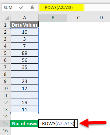
Press ENTER key here, and it will return the count of rows.
The final result is shown below:
Explanation:
When we pass the range of cells, it gives you the count of cells you selected.
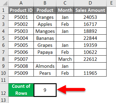
Example #4
We have given below product details:
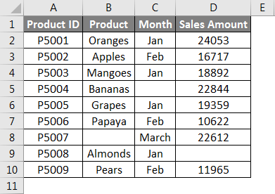
Now we will pass the range of the given dataset within the function like the below screenshot:
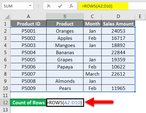
Press ENTER key, which will give you the count of rows containing data in the passing range.
The final result is given below:
Example #5
We have given some raw data.
Some cell values are missing here, so now, for counting the rows, we will apply the function shown in the below screenshot:
Hit the Enter key, and it will return the count of rows having data.
The final result is given below:
Example #6
We have given a company employee data where some details are missing:
Now apply the ROWS function to count the row containing data of employees:
Hit the Enter key to get the final rows
Things to Remember About Row Count in Excel
- When you click on the column heading for counting the rows, it will give you the count which contains data.
- If you pass a range of cells, it will return the number of cells that you have selected.
- The status bar won’t show you anything if the column contains the data only in one cell. That is, the status bar stays blank.
- If the data are given in the table form, then for counting the rows, you can pass the table range within the ROWS function.
- You can also do the setting of the message in the status bar. Do right-click on the status bar and click the item you want to see or remove.
Recommended Articles
This article has been a guide to Row Count in Excel. Here we discussed How to Count the Rows, practical examples, and a downloadable Excel template. You can also go through our other suggested articles–
- COUNTA Function in Excel
- Count Function in Excel
- ROWS Function in Excel
- Add Rows in Excel Shortcut
Содержание
- Определение количества строк
- Способ 1: указатель в строке состояния
- Способ 2: использование функции
- Способ 3: применение фильтра и условного форматирования
- Вопросы и ответы

При работе в Excel иногда нужно подсчитать количество строк определенного диапазона. Сделать это можно несколькими способами. Разберем алгоритм выполнения этой процедуры, используя различные варианты.
Определение количества строк
Существует довольно большое количество способов определения количества строк. При их использовании применяются различные инструменты. Поэтому нужно смотреть конкретный случай, чтобы выбрать более подходящий вариант.
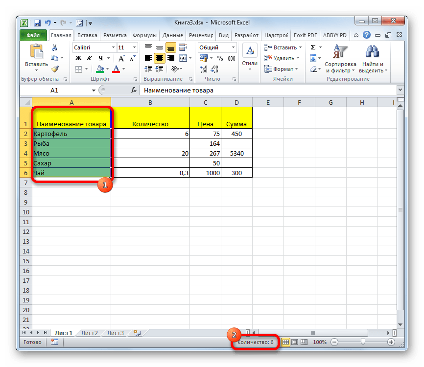
Способ 1: указатель в строке состояния
Самый простой способ решить поставленную задачу в выделенном диапазоне – это посмотреть количество в строке состояния. Для этого просто выделяем нужный диапазон. При этом важно учесть, что система считает каждую ячейку с данными за отдельную единицу. Поэтому, чтобы не произошло двойного подсчета, так как нам нужно узнать количество именно строк, выделяем только один столбец в исследуемой области. В строке состояния после слова «Количество» слева от кнопок переключения режимов отображения появится указание фактического количества заполненных элементов в выделенном диапазоне.
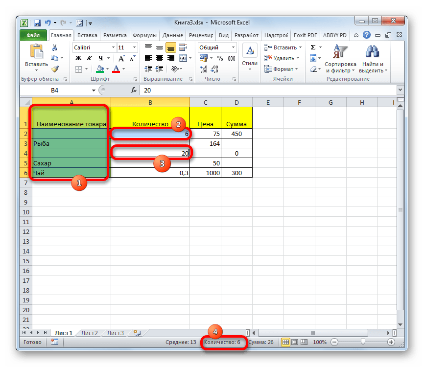
Правда, случается и такое, когда в таблице нет полностью заполненных столбцов, при этом в каждой строке имеются значения. В этом случае, если мы выделим только один столбец, то те элементы, у которых именно в той колонке нет значений, не попадут в расчет. Поэтому сразу выделяем полностью конкретный столбец, а затем, зажав кнопку Ctrl кликаем по заполненным ячейкам, в тех строчках, которые оказались пустыми в выделенной колонке. При этом выделяем не более одной ячейки на строку. Таким образом, в строке состояния будет отображено количество всех строчек в выделенном диапазоне, в которых хотя бы одна ячейка заполнена.
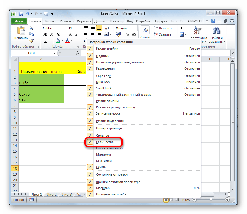
Но бывают и ситуации, когда вы выделяете заполненные ячейки в строках, а отображение количества на панели состояния так и не появляется. Это означает, что данная функция просто отключена. Для её включения кликаем правой кнопкой мыши по панели состояния и в появившемся меню устанавливаем галочку напротив значения «Количество». Теперь численность выделенных строк будет отображаться.
Способ 2: использование функции
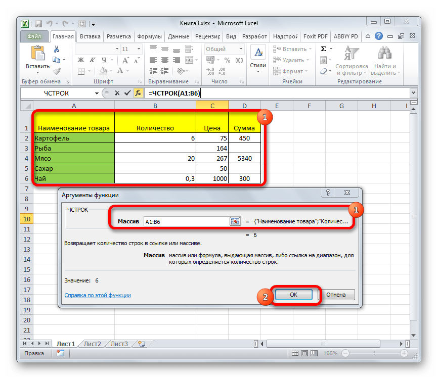
Но, вышеуказанный способ не позволяет зафиксировать результаты подсчета в конкретной области на листе. К тому же, он предоставляет возможность посчитать только те строки, в которых присутствуют значения, а в некоторых случаях нужно произвести подсчет всех элементов в совокупности, включая и пустые. В этом случае на помощь придет функция ЧСТРОК. Её синтаксис выглядит следующим образом:
=ЧСТРОК(массив)
Её можно вбить в любую пустую ячейку на листе, а в качестве аргумента «Массив» подставить координаты диапазона, в котором нужно произвести подсчет.
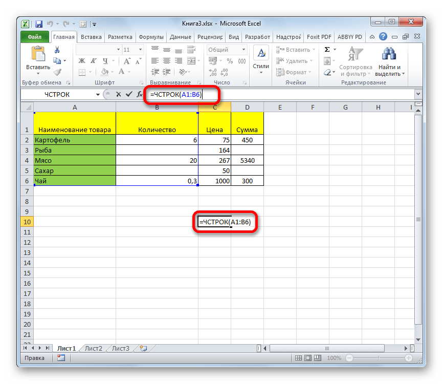
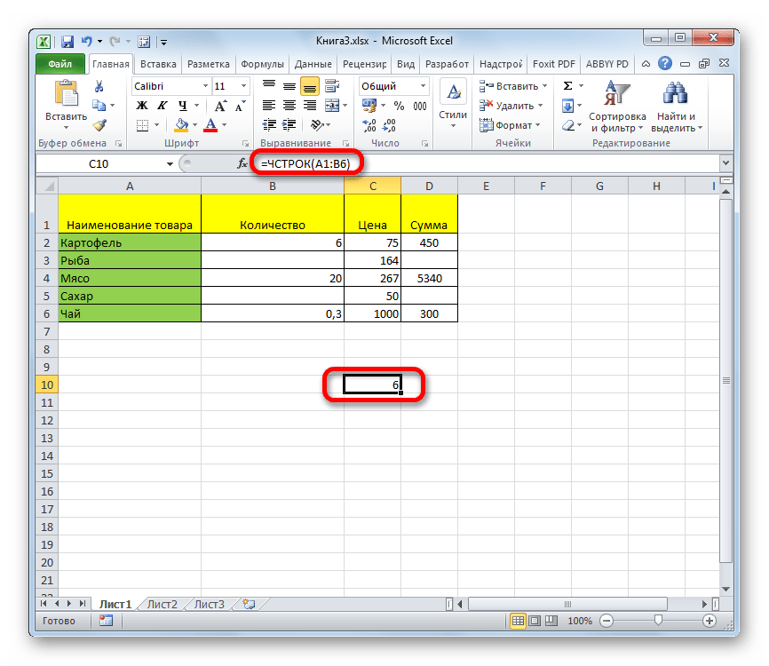
Для вывода результата на экран достаточно будет нажать кнопку Enter.


Причем подсчитываться будут даже полностью пустые строки диапазона. Стоит заметить, что в отличие от предыдущего способа, если вы выделите область, включающую несколько столбцов, то оператор будет считать исключительно строчки.
Пользователям, у которых небольшой опыт работы с формулами в Экселе, проще работать с данным оператором через Мастер функций.
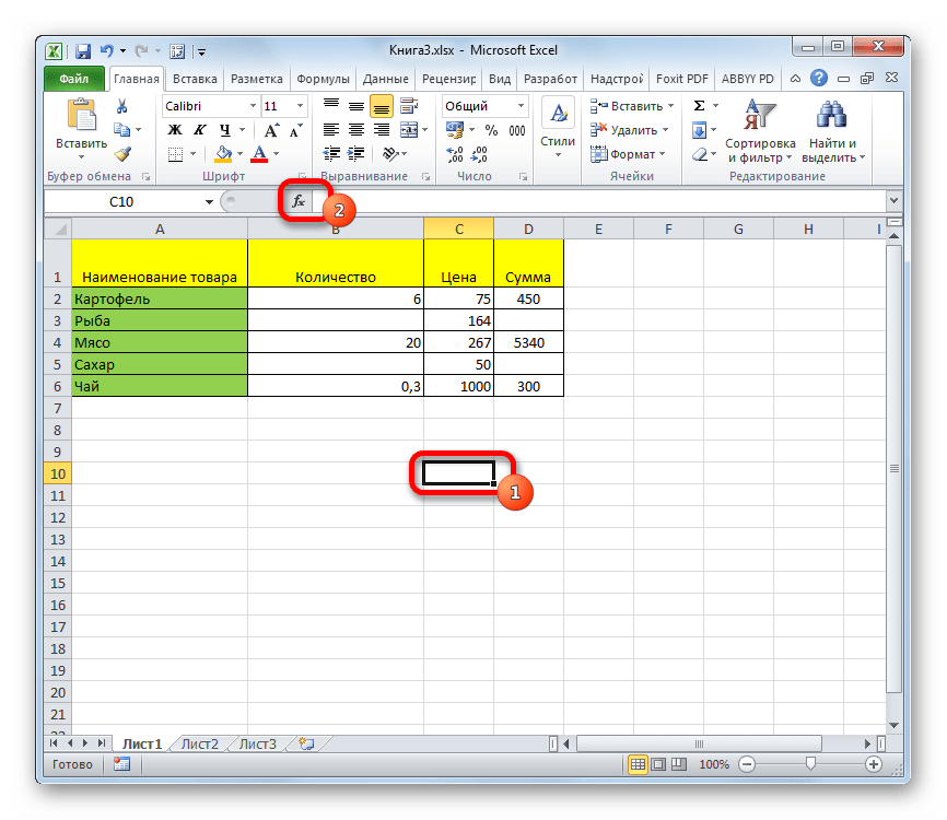
- Выделяем ячейку, в которую будет производиться вывод готового итога подсчета элементов. Жмем на кнопку «Вставить функцию». Она размещена сразу слева от строки формул.
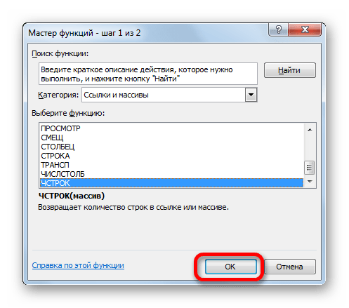
- Запускается небольшое окно Мастера функций. В поле «Категории» устанавливаем позицию «Ссылки и массивы» или «Полный алфавитный перечень». Ищем значение «ЧСТРОК», выделяем его и жмем на кнопку «OK».
- Открывается окно аргументов функции. Ставим курсор в поле «Массив». Выделяем на листе тот диапазон, количество строк в котором нужно подсчитать. После того, как координаты этой области отобразились в поле окна аргументов, жмем на кнопку «OK».
- Программа обрабатывает данные и выводит результат подсчета строк в предварительно указанную ячейку. Теперь этот итог будет отображаться в данной области постоянно, если вы не решите удалить его вручную.
Урок: Мастер функций в Экселе
Способ 3: применение фильтра и условного форматирования
Но бывают случаи, когда нужно подсчитать не все строки диапазона, а только те, которые отвечают определенному заданному условию. В этом случае на помощь придет условное форматирование и последующая фильтрация
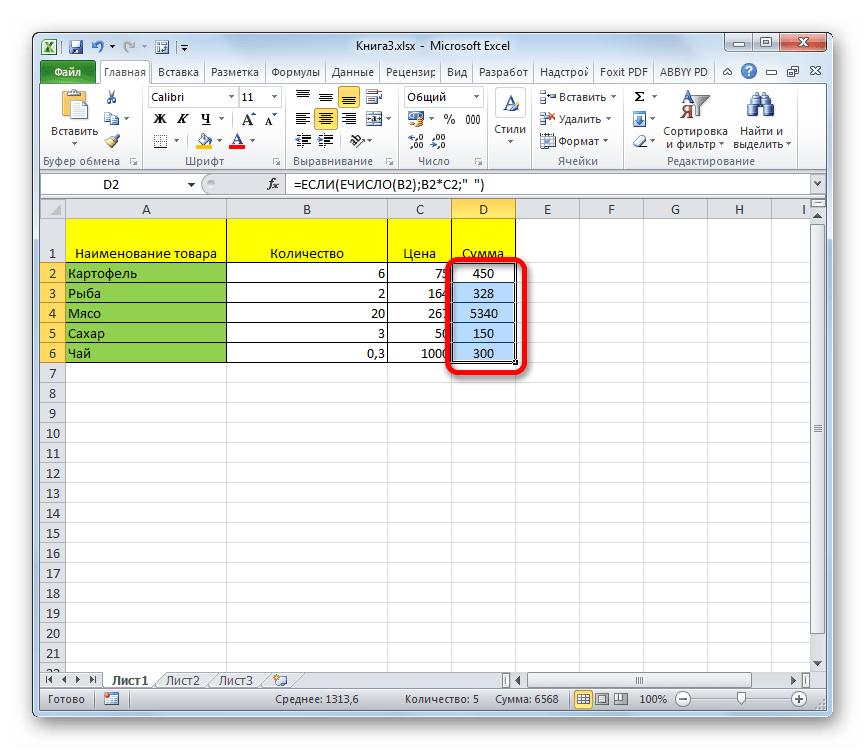
- Выделяем диапазон, по которому будет производиться проверка на выполнение условия.
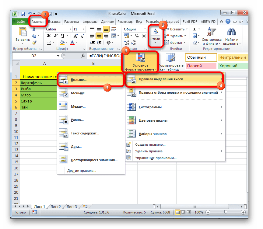
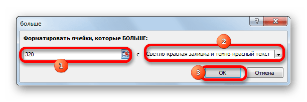
- Переходим во вкладку «Главная». На ленте в блоке инструментов «Стили» жмем на кнопку «Условное форматирование». Выбираем пункт «Правила выделения ячеек». Далее открывается пункт различных правил. Для нашего примера мы выбираем пункт «Больше…», хотя для других случаев выбор может быть остановлен и на иной позиции.
- Открывается окно, в котором задается условие. В левом поле укажем число, ячейки, включающие в себя значение больше которого, окрасятся определенным цветом. В правом поле существует возможность этот цвет выбрать, но можно и оставить его по умолчанию. После того, как установка условия завершена, жмем на кнопку «OK».
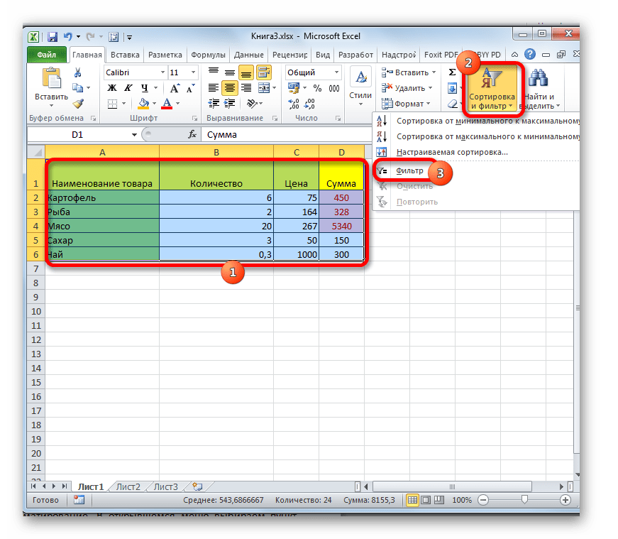
- Как видим, после этих действий ячейки, удовлетворяющие условию, были залиты выбранным цветом. Выделяем весь диапазон значений. Находясь во все в той же вкладке «Главная», кликаем по кнопке «Сортировка и фильтр» в группе инструментов «Редактирование». В появившемся списке выбираем пункт «Фильтр».
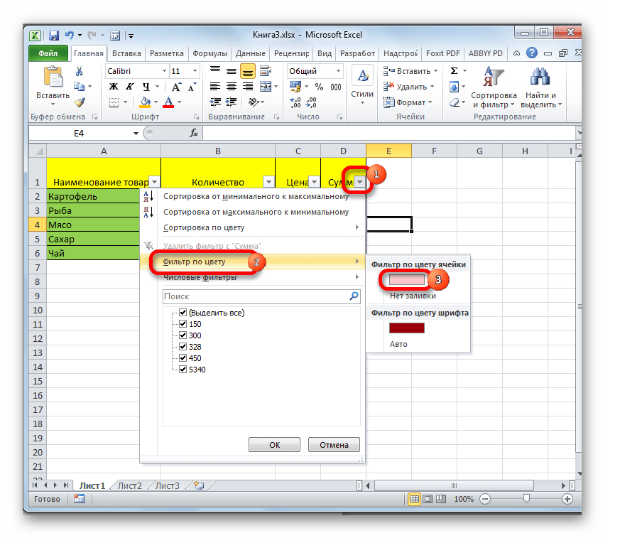
- После этого в заглавиях столбцов появляется значок фильтра. Кликаем по нему в том столбце, где было проведено форматирование. В открывшемся меню выбираем пункт «Фильтр по цвету». Далее кликаем по тому цвету, которым залиты отформатированные ячейки, удовлетворяющие условию.
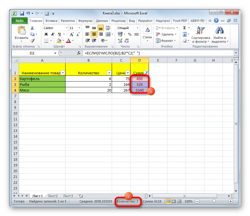
- Как видим, не отмеченные цветом ячейки после данных действий были спрятаны. Просто выделяем оставшийся диапазон ячеек и смотрим на показатель «Количество» в строке состояния, как и при решении проблемы первым способом. Именно это число и будет указывать на численность строк, которые удовлетворяют конкретному условию.
Урок: Условное форматирование в Эксель
Урок: Сортировка и фильтрация данных в Excel
Как видим, существует несколько способов узнать количество строчек в выделенном фрагменте. Каждый из этих способов уместно применять для определенных целей. Например, если нужно зафиксировать результат, то в этом случае подойдет вариант с функцией, а если задача стоит подсчитать строки, отвечающие определенному условию, то тут на помощь придет условное форматирование с последующей фильтрацией.