
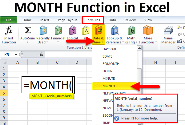
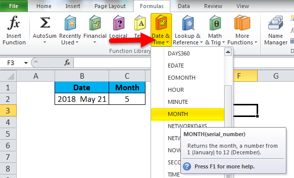
Excel for Microsoft 365 Excel for Microsoft 365 for Mac Excel for the web Excel 2021 Excel 2021 for Mac Excel 2019 Excel 2019 for Mac Excel 2016 Excel 2016 for Mac Excel 2013 Excel 2010 Excel 2007 Excel for Mac 2011 Excel Starter 2010 More…Less
This article describes the formula syntax and usage of the MONTH function in Microsoft Excel.
Description
Returns the month of a date represented by a serial number. The month is given as an integer, ranging from 1 (January) to 12 (December).
Syntax
MONTH(serial_number)
The MONTH function syntax has the following arguments:
-
Serial_number Required. The date of the month you are trying to find. Dates should be entered by using the DATE function, or as results of other formulas or functions. For example, use DATE(2008,5,23) for the 23rd day of May, 2008. Problems can occur if dates are entered as text.
Remarks
Microsoft Excel stores dates as sequential serial numbers so they can be used in calculations. By default, January 1, 1900 is serial number 1, and January 1, 2008 is serial number 39448 because it is 39,448 days after January 1, 1900.
Values returned by the YEAR, MONTH and DAY functions will be Gregorian values regardless of the display format for the supplied date value. For example, if the display format of the supplied date is Hijri, the returned values for the YEAR, MONTH and DAY functions will be values associated with the equivalent Gregorian date.
Example
Copy the example data in the following table, and paste it in cell A1 of a new Excel worksheet. For formulas to show results, select them, press F2, and then press Enter. If you need to, you can adjust the column widths to see all the data.
|
Date |
||
|---|---|---|
|
15-Apr-11 |
||
|
Formula |
Description |
Result |
|
=MONTH(A2) |
Month of the date in cell A2 |
4 |
See Also
DATE function
Add or subtract dates
Date and time functions (reference)
Need more help?
Want more options?
Explore subscription benefits, browse training courses, learn how to secure your device, and more.
Communities help you ask and answer questions, give feedback, and hear from experts with rich knowledge.
To find the number of months or days between two dates, type into a new cell: =DATEDIF(A1,B1,”M”) for months or =DATEDIF(A1,B1,”D”) for days.
Contents
- 1 What is the formula for month in Excel?
- 2 How do I calculate month and year in Excel?
- 3 How do I calculate days and months in Excel?
- 4 How do I convert weeks to months in Excel?
- 5 How do you calculate beginning of month in Excel?
- 6 How are days and months calculated?
- 7 How do you calculate week of month?
- 8 How do you calculate weeks into months?
- 9 How do I convert weekly data to monthly in Excel?
- 10 How do I get the start and end of the month in Excel?
- 11 How do I calculate month ending date in Excel?
- 12 What is the Eomonth function in Excel?
- 13 How do I calculate weeks in Excel?
- 14 How do I use Isoweeknum in Excel?
- 15 How do I change the Weeknum in Excel?
- 16 How do I find the first Monday of the month in Excel?
- 17 Is 12 weeks and 3 months the same?
- 18 How many months are in a?
- 19 How many work weeks are in a month?
- 20 How do I convert monthly data to quarterly in Excel?
What is the formula for month in Excel?
How to extract month name from date in Excel. In case you want to get a month name rather than a number, you use the TEXT function again, but with a different date code: =TEXT(A2, “mmm”) – returns an abbreviated month name, as Jan – Dec. =TEXT(A2,”mmmm”) – returns a full month name, as January – December.
How do I calculate month and year in Excel?
- Click on a blank cell where you want the new date format to be displayed (D2)
- Type the formula: =B2 & “-“ & C2. Alternatively, you can type: =MONTH(A2) & “-” & YEAR(A2).
- Press the Return key.
- This should display the original date in our required format.
How do I calculate days and months in Excel?
Calculate elapsed year, month and days
Select a blank cell which will place the calculated result, enter this formula =DATEDIF(A2,B2,”Y”) & ” Years, ” & DATEDIF(A2,B2,”YM”) & ” Months, ” & DATEDIF(A2,B2,”MD”) & ” Days”, press Enter key to get the result.
How do I convert weeks to months in Excel?
Click the cell that you want to get month and type this formula =CHOOSE(MONTH(DATE(A2,1,B2*7-2)-WEEKDAY(DATE(B2,1,3))),”January”, “February”, “March”, “April”, “May”, “June”, “July”, “August”, “September”, “October”, “November”, “December”) into it, then press Enter key to get the result, and then drag auto fill to
How do you calculate beginning of month in Excel?
To get the first day of the months, we need to:
- Go to cell B2. Click on it with the mouse.
- Input the formula =A2-DAY(A2)+1 to the function box in B2.
- Press Enter.
How are days and months calculated?
To convert a month measurement to a day measurement, multiply the time by the conversion ratio. The time in days is equal to the months multiplied by 30.436875.
How do you calculate week of month?
Observe the number of weeks in the 12 different months of a year. In order to calculate the number of weeks in a month, we need to count the number of days in the month and divide that number by 7 (1 week = 7 days).
How do you calculate weeks into months?
How to Convert Weeks to Months. To convert a week measurement to a month measurement, multiply the time by the conversion ratio. The time in months is equal to the weeks multiplied by 0.229984.
How do I convert weekly data to monthly in Excel?
7. Click a cell in the date column of the pivot table that Excel created in the spreadsheet. Right-click and select “Group,” then “Days.” Enter “7” in the “Number of days” box to group by week. Click “OK” and verify that you have correctly converted daily data to weekly data.
How do I get the start and end of the month in Excel?
In this example, there is a January start date in cell A2 and a June end date in cell B2. To find the number of dates between the start date and end date, use this formula in cell C2: =B2-A2.
How do I calculate month ending date in Excel?
Use a formula to find the end date of each month may be very easy for every Excel user. Also, you can use this formula =EOMONTH(A2,0) to get the month’s end date. (You need to format the result cells as Date format before entering this formula.)
What is the Eomonth function in Excel?
What is the EOMONTH Function? The EOMONTH Function is categorized under Excel Date/Time functions. This cheat sheet covers 100s of functions that are critical to know as an Excel analyst. The function helps to calculate the last day of the month after adding a specified number of months to a date.
How do I calculate weeks in Excel?
To find out how many weeks there are between two dates, you can use the DATEDIF function with “D” unit to return the difference in days, and then divide the result by 7. Where A2 is the start date and B2 is the end date of the period you are calculating.
How do I use Isoweeknum in Excel?
This article describes the formula syntax and usage of the ISOWEEKNUM function in Microsoft Excel.
Example.
| Date | ||
|---|---|---|
| Formula | Description | Result |
| =ISOWEEKNUM(A2) | Number of the week in the year that 3/9/2012 occurs, based on weeks beginning on the default, Monday (10). | 10 |
How do I change the Weeknum in Excel?
On the other hand, you can also apply the WEEKNUM function to convert a date to corresponding week number. 1. Select a blank cell you will return the week number, enter this formula: =WEEKNUM(B1,1), and press the Enter key.
How do I find the first Monday of the month in Excel?
How to find the first weekday of the month in Excel
- =EOMONTH(A1,-1)+1+CHOOSE(WEEKDAY(EOMONTH(A1,-1)+1,2),0,0,0,0,0,2,1) This formula will work with Excel 2007 and later versions.
- =EOMONTH(A1,-1)+1.
- +CHOOSE(WEEKDAY(EOMONTH(A1,-1)+1,2),0,0,0,0,0,2,1)
- =CHOOSE(2,”Oranges”,”Apples”,”Pears”)
Is 12 weeks and 3 months the same?
12 Weeks Pregnant Is How Many Months? At 12 weeks pregnant, you’re about three months pregnant. Remember, pregnancy is 40 weeks long, which doesn’t break down cleanly into nine months.
How many months are in a?
Months
| Month Number | Month | Days in Month |
|---|---|---|
| 1 | January | 31 |
| 2 | February | 28 (29 in leap years) |
| 3 | March | 31 |
| 4 | April | 30 |
How many work weeks are in a month?
There are about 4.3 weeks per month.
How do I convert monthly data to quarterly in Excel?
If we divide the month by 3 and then round the value up to nearest integer we will get the Quarter. So, A formula like =ROUNDUP(MONTH(B4)/3,0) should tell us the quarter for the month in the cell B4.
Purpose
Get month as a number (1-12) from a date
Return value
A number between 1 and 12.
Usage notes
The MONTH function extracts the month from a given date as a number between 1 to 12. For example, given the date «June 12, 2021», the MONTH function will return 6 for June. MONTH takes just one argument, serial_number, which must be a valid Excel date.
Dates can be supplied to the MONTH function as text (e.g. «13-Aug-2021») or as native Excel dates, which are large serial numbers. To create a date value from scratch with separate year, month, and day inputs, use the DATE function.
The MONTH function will «reset» every 12 months (like a calendar). To work with month durations larger than 12, use a formula to calculate months between dates.
The MONTH function returns a number. If you need the month name, see this example.
Examples
To use the MONTH function, supply a date:
=MONTH("23-Aug-2012") // returns 8
=MONTH("11-May-2019") // returns 5
With the date «September 15, 2017» in cell A1, MONTH returns 9:
=MONTH(A1) // returns 9
You can use the MONTH function to extract a month number from a date into a cell, or to feed a month number into another function like the DATE function. The formula below extracts the month from the date in cell A1 and uses the TODAY and DATE functions to create a date on the first day of the same month in the current year.
=DATE(YEAR(TODAY(),MONTH(A1),1) // same month current year
See below for more examples of formulas that use the MONTH function.
Note: dates are serial numbers in Excel, and begin on January 1, 1900. Dates before 1900 are not supported. To display date values in a human-readable date format, apply the number format of your choice.
Notes
- MONTH will return #VALUE! if a date is not recognized.
- MONTH will return #NUM! if a date is supplied as a number that is out of range (i.e. -1).
The MONTH function in Excel is a date function used to find the month for a given date in a date format. This function takes an argument in a date format, and the result is in integer format. This function’s value is in the range of 1-12 as there are only twelve months in a year. The method to use this function is as follows =MONTH( serial_number). The argument provided to this function should be in a recognizable date format of Excel.
For example, =MONTH(A1) – returns the month of a date in A1.
=MONTH(DATE(2020,6,10)) – returns 6 corresponding to June.
Also, =MONTH(“10-June-2020”) – returns number 6 too.
The MONTH function in Excel gives the month from its date. It returns the month number ranging from 1 to 12.
Table of contents
- MONTH Function in Excel
- MONTH Formula in Excel
- MONTH in Excel – Illustration
- How to Use MONTH Function in Excel?
- MONTH in Excel Example #1
- MONTH in Excel Example #2
- MONTH in Excel Example #3
- MONTH in Excel Example #4
- MONTH in Excel Example #5
- Things to remember about a MONTH in Excel
- MONTH Excel Function Video
- Recommended Articles
MONTH Formula in Excel
Below is the MONTH Formula in Excel.

Or
MONTH( date )
MONTH in Excel – Illustration
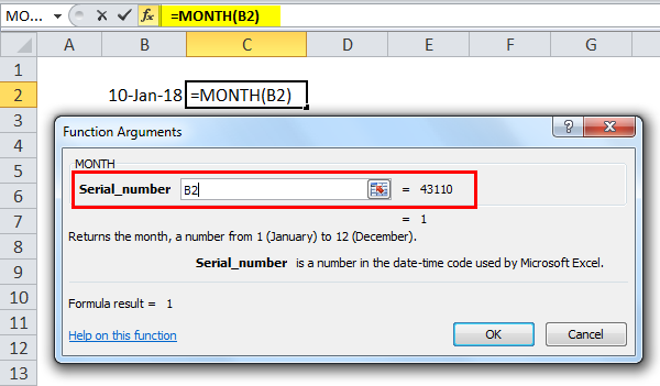
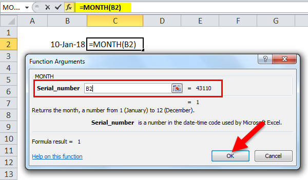
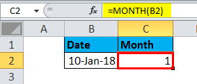
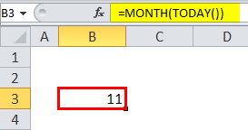
Suppose a date (10 August, 18) is given in cell B3. You want to find the month in Excel of the given date in numbers.

You can use the MONTH formula in Excel given below:
= MONTH (B3)

Press the “Enter” key. The MONTH function in Excel will return 8.

You can also use the following MONTH formula in Excel:
= MONTH (“10 Aug 2018”)

Press the “Enter” key. The MONTH function will also return the same value.

The date 10 Aug 2018 refers to a value 43322 in Excel. You can also use this value directly as input to the MONTH function. The MONTH formula in Excel would be:
= MONTH (43322)

MONTH function in Excel will return 8.

Alternatively, you can also use the date in another format:
= MONTH (“10-Aug-2018”)

Excel MONTH function will also return 8.

Let us look at examples of where and how to use the MONTH function in Excel in various scenarios.
How to Use MONTH Function in Excel?
The MONTH function in Excel is very simple and easy to use. Let us understand the working of a MONTH in excel by some examples.
serial_number: a valid date for which the month number is to be identified
The input date must be a valid Excel dateThe date function in excel is a date and time function representing the number provided as arguments in a date and time code. The result displayed is in date format, but the arguments are supplied as integers.read more. The dates in Excel are stored as serial numbers. For example, the date Jan 1, 2010, equals the serial number 40179 in Excel. The MONTH formula in Excel takes as input both the date directly or the serial number of the date. It is to be noted here that Excel does not recognize dates earlier than 1/1/1900.
Returns
The MONTH function in Excel always returns a number ranging from 1 to 12. This number corresponds to the month of the input date.
You can download this MONTH Function Excel Template here – MONTH Function Excel Template
MONTH in Excel Example #1
Suppose you have a list of dates given in the cells B3: B7, as shown below. You want to find the month name of each of these given dates.

You can do so using the following MONTH formula in Excel:
= CHOOSE ((MONTH(B3)), “Jan”, “Feb”, “Mar”, “Apr”, “May”, “Jun”, “Jul”, “Aug”, “Sep”, “Oct”, “Nov”, “Dec”)

MONTH (B3) will return 1.
CHOOSE (1, …..) will choose the 1st option of the given 12, Jan here.
So, the MONTH function in Excel will return Jan as a result.

Similarly, you can drag it for the rest of the cells.

Alternatively, you can use the following MONTH formula in Excel:
= TEXT (B3, “mmm”)

The MONTH function will return Jan as a result.

MONTH in Excel Example #2
Suppose you have month names (say in “mmm” format) given in cells B4: B15.
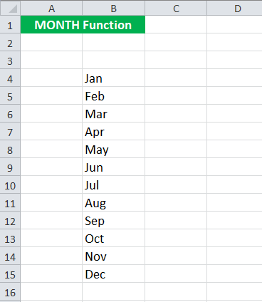
Now, you want to convert these names to the month in numbers.
You can use the following MONTH in Excel:
= MONTH ( DATEVALUE( B4 & ” 1”)


For Jan, the MONTH in Excel will return 1. For Feb, it will return 2 and so on.

MONTH in Excel Example #3
Suppose you have a list of holidays given in cells B3: B9 in a date-wise manner, as shown below.
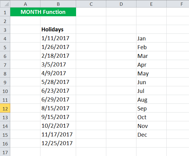
Now, you want to calculate the number of holidays each month. To do so, you can use the following MONTH formula in Excel for the first month given in E4:
= SUMPRODUCT( –( MONTH( $B$4:$B$16 ) = MONTH( DATEVALUE( E4 & ” 1″)) ) )

Then, drag it to the rest of the cells.
Let us look at the MONTH function in Excel detail:
- MONTH( $B$4:$B$16 ) will check the month of the dates provided in cell range B4:B16 in a number format. The MONTH function in Excel will return {1; 1; 2; 3; 4; 5; 6; 6; 8; 9; 10; 11; 12}
- MONTH( DATEVALUE( E4 & ” 1″) will give the month in number corresponding to cell E4 (see example 2). The MONTH function in Excel will return 1 for January
- SUMPRODUCT in ExcelThe SUMPRODUCT excel function multiplies the numbers of two or more arrays and sums up the resulting products.read more (– (…) = (..) ) will match the month given in B4:B16 with January (=1) and will add one each time when it is true.
Since January appears twice in the given data, the MONTH function in Excel will return 2.

Similarly, you can do for the rest of the cells.

MONTH in Excel Example #4
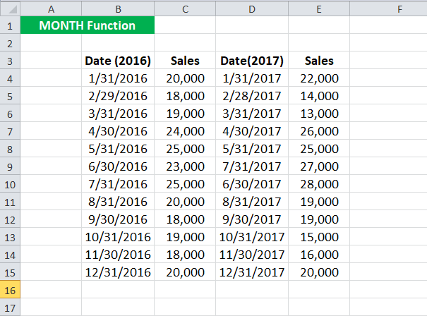
Suppose you have sales data for the past two years. The data was collected on the last date of the month. The data was manually entered, so there could be a mismatch in the data. You should compare the sales between 2016 and 2017 for each month.
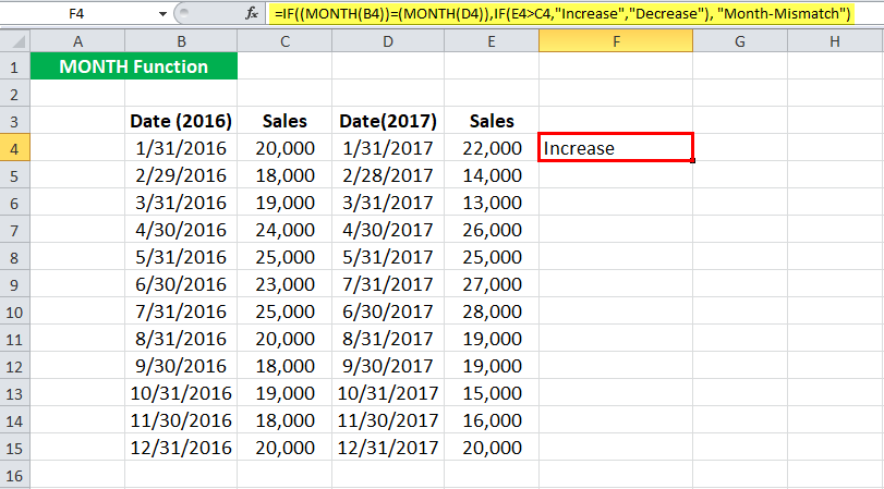
To check if the months are the same and then compare the sales, you can use the MONTH formula in Excel:
=IF( (MONTH(B4)) = (MONTH(D4) ), IF( E4 > C4, “Increase”, “Decrease” ), “Month-Mismatch” )

For the first entry, the MONTH function in Excel will return “Increase.”
Let us look at the MONTH in Excel in detail:
If the MONTH of B4 (for 2016) is equal to the MONTH given in D4 (for 2017),
- The MONTH function in Excel will check if the sales for the given month in 2017 are greater than that in 2016.
- If it is greater, it will return “Increase.”
- Else, it will return to “Decrease.”
If the MONTH of B4 (for 2016) is not equal to the MONTH given in D4 (for 2017),
- The MONTH function in Excel will return “Mismatch.”
Similarly, you can do for the rest of the cells.

You could also add another condition to check if the sales are equal and return “Constant.”
MONTH in Excel Example #5
Suppose you work in your company’s sales department and have date-wise data of how many products were sold on a particular date for the previous year, as shown below.

Now, you want to club the number of products monthly. To do so, you use the following MONTH formula in Excel:
= SUMPRODUCT(– ( EXACT( F4, MONTH( $B$4:$B$17 ))), $C$4:$C$17 )
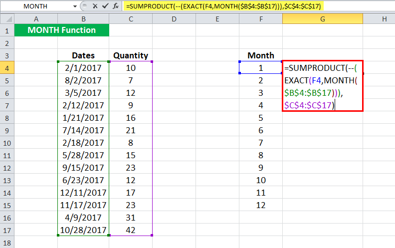
For the first cell, the MONTH function in Excel will return 16.

Then, drag it to the rest of the cells.

Let us look at the MONTH in Excel in detail:
= SUMPRODUCT(– ( EXACT( F4, MONTH( $B$4:$B$17 ))), $C$4:$C$17 )
- MONTH( $B$4:$B$17 ) will give the month of the cells in B4: B17. MONTH function in Excel will return a matrix {2; 8; 3; 2; 1; 7; 2; 5; 9; 6; 12; 11; 4; 10}
- EXACT( F4, MONTH( $B$4:$B$17 )) will match the month in F4 ( 1 here) with the matrix and will return another matrix with TRUE when it is a match or FALSE otherwise. For the 1st month, it will return {FALSE; FALSE; FALSE; FALSE; TRUE; FALSE; FALSE; FALSE; FALSE; FALSE; FALSE; FALSE; FALSE; FALSE}
- SUMPRODUCT (– (..), $C$4:$C$17) will sum the values in C4:C17 when the corresponding value in the matrix is “TRUE.”
The MONTH function in Excel will return 16 for January.

Things to remember about a MONTH in Excel
- The MONTH function returns the month of the given date or serial number.
- Excel MONTH function is given #VALUE! Error when it cannot recognize the date.
- The Excel MONTH function accepts dates only after 1 Jan 1900. It will provide the #VALUE! Error when the input date is earlier than 1 Jan 1900.
- The MONTH function in Excel returns the month in number format only. Therefore, its output is always a number between 1 and 12.
MONTH Excel Function Video
Recommended Articles
This article is a guide to MONTH Function in Excel. We discuss the MONTH formula in Excel and how to use the MONTH function, along with Excel examples and downloadable Excel templates. You may also look at these useful functions in Excel: –
- EDATE Function in ExcelEDATE is a date and time function in excel which adds a given number of months into a date and gives us a date in a numerical format of date. It takes dates and integers as input, the output returned by this function is also a date value. read more
- VBA MONTH VBA Month Function is an inbuilt function that is used to extract the month from a date. The output of this function is an integer ranging from 1 to 12. Only the month number is extracted from the supplied date value by this function.read more
- EOMONTH in ExcelEOMONTH is a worksheet date function in excel which calculates the end of the month for the given date by adding a specified number of months to the arguments. This function takes two arguments: the date and another as integer, and the output is in the date format.read more
- FREQUENCY Excel FunctionThe FREQUENCY function in Excel calculates the number of times a data values occurs within a given range of values and returns a vertical array of numbers corresponding to each value’s frequency within a range.read more
If you manage multiple projects, you would have a need to know how many months have passed between two dates. Or, if you’re in the planning phase, you may need to know the same for the start and end date of a project.
There are multiple ways to calculate the number of months between two dates (all using different formulas).
In this tutorial, I will give you some formulas that you can use to get the number of months between two dates.
So let’s get started!
Using DATEDIF Function (Get Number of Completed Months Between Two Dates)
It’s unlikely that you will get the dates that have a perfect number of months. It’s more likely to be some number of months and some days that are covered by the two dates.
For example, between 1 Jan 2020 and 15 March 2020, there are 2 months and 15 days.
If you only want to calculate the total number of months between two dates, you can use the DATEDIF function.
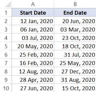
Suppose you have a dataset as shown below where you only want to get the total number of months (and not the days).
Below is the DATEDIF formula that will do that:
=DATEDIF(A2,B2,"M")
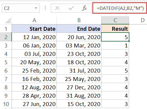
The above formula will give you only the total number of completed months between two dates.
DATEDIF is one of the few undocumented functions in Excel. When you type the =DATEDIF in a cell in Excel, you would not see any IntelliSense or any guidance on what arguments it can take. So, if you’re using DATEDIF in Excel, you need to know the syntax.
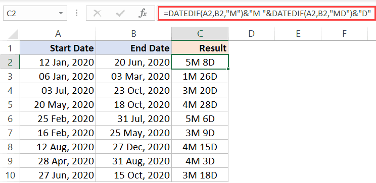
In case you want to get the total number of months as well as days between two dates, you can use the below formula:
=DATEDIF(A2,B2,"M")&"M "&DATEDIF(A2,B2,"MD")&"D"
Note: DATEDIF function will exclude the start date when counting the month numbers. For example, if you start a project on 01 Jan and it ends on 31 Jan, the DATEDIF function will give the number of months as 0 (as it doesn’t count the start date and according to it only 30 days in January have been covered)
Using YEARFRAC Function (Get Total Months Between Two Dates)
Another method to get the number of months between two specified dates is by using the YEARFRAC function.
The YEARFRAC function will take a start date and end date as input arguments and it will give you the number of years that have passed during these two dates.
Unlike the DATEDIF function, the YEARFRAC function will give you the values in decimal in case a year has not elapsed between the two dates.
For example, if my start date is 01 Jan 2020 and end date is 31 Jan 2o20, the result of the YEARFRAC function will be 0.833. Once you have the year value, you can get the month value by multiplying this with 12.
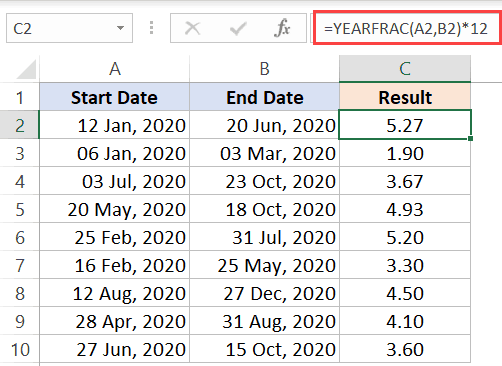
Suppose you have the dataset as shown below and you want to get the number of months between the start and end date.
Below is the formula that will do this:
=YEARFRAC(A2,B2)*12
This will give you the months in decimals.
In case you only want to get the number of complete months, you can wrap the above formula in INT (as shown below):
=INT(YEARFRAC(A2,B2)*12)
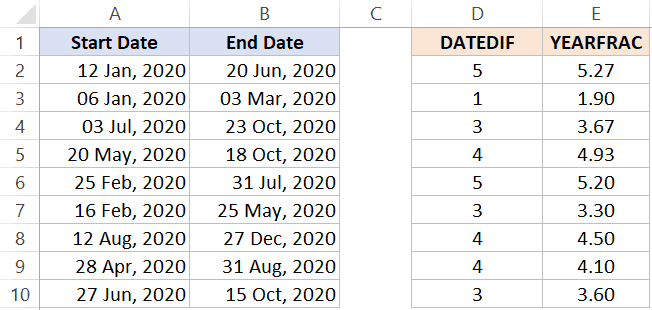
Another major difference between the DATEDIF function and YEARFRAC function is that the YEARFRAC function will consider the start date as a part of the month. For example, if the start date is 01 Jan and end date is 31 Jan, the result from the above formula would be 1
Below is a comparison of the results you get from DATEDIF and YEARFRAC.
Using the YEAR and MONTH Formula (Count All Months when the Project was Active)
If you want to know the total months that are covered between the start and end date, then you can use this method.
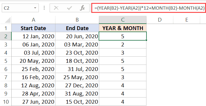
Suppose you have the dataset as shown below:
Below is the formula that will give you the number of months between the two dates:
=(YEAR(B2)-YEAR(A2))*12+MONTH(B2)-MONTH(A2)
This formula uses the YEAR function (which gives you the year number using the date) and the MONTH function (which gives you the month number using the date).
The above formula also completely ignores the month of the start date.
For example, if your project starts on 01 Jan and ends on 20 Feb, the formula shown below will give you the result as 1, as it completely ignores the start date month.
In case you want it to count the month of the start date as well, you can use the below formula:
=(YEAR(B2)-YEAR(A2))*12+(MONTH(B2)-MONTH(A2)+1)
You may want to use the above formula when you want to know-how in how many months was this project active (which means that it could count the month even if the project was active for only 2 days in the month).
So these are three different ways to calculate months between two dates in Excel. The method you choose would be based on what you intend to calculate (below is a quick summary):
- Use the DATEDIF function method if you want to get the total number of completed months in between two dates (it ignores the start date)
- Use the YEARFRAC method when you want to get the actual value of months elapsed between tow dates. It also gives the result in decimal (where the integer value represents the number of full months and decimal part represents the number of days)
- Use the YEAR and MONTH method when you want to know how many months are covered in between two dates (even when the duration between the start and the end date is only a few days)
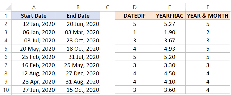
Below is how each formula covered in this tutorial will count the number of months between two dates:
Hope you found this Excel tutorial useful.
You may also like the following Excel tips and tutorials:
- How to Calculate the Number of Days Between Two Dates in Excel
- How to Remove Time from Date/Timestamp in Excel
- Convert Time to Decimal Number in Excel (Hours, Minutes, Seconds)
- How to Quickly Insert Date and Timestamp in Excel
- Convert Date to Text in Excel
- How to SUM values between two dates in Excel
- How to Add Months to Date in Excel
- How to Calculate Years of Service in Excel (Easy Formulas)
- How to Make an Interactive Calendar in Excel? (FREE Template)
Excel MONTH Function (Table of Contents)
- MONTH in Excel
- MONTH Formula in Excel
- How to Use MONTH Function in Excel?
MONTH in Excel
The month function in excel is one of the simplest functions to understand, which only returns a month out of any selected dates. We can either enter the select the cell containing a date or enter to the month number we want to see. But using the Month function by selecting any date and getting the month number out of that is the best way to use it.
MONTH Formula in Excel:
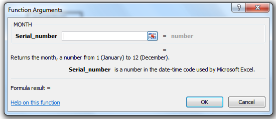
The Formula for the MONTH Function in Excel is as follows.
The MONTH function uses only one argument where the serial number argument is the date that you want to return the month.
NOTE: It is recommended that dates should be supplied to Excel functions as either, Serial numbers or Reference to cells containing dates or Date values returned from other Excel formulas.
DAY Formula in Excel:
The Formula for the DAY Function in Excel is as follows.
Arguments :
date_value/ Serial_number: A valid date to return the day.
Returns:
The DAY function returns a numeric value between 1 and 31.
YEAR Formula in Excel:
The Formula for the YEAR Function in Excel is as follows.
Arguments:
date_value/Serial_number: A valid date to return the month.
Returns:
The YEAR function returns a numeric value between 1999 and 9999.
Steps to Use Month Function in Excel
MONTH Function in Excel can be used as part of a formula in a cell of a worksheet. Let’s consider the below example for good understanding. We cannot enter 10/05/2018 directly into the cell. Instead,d we need to enter “10/05/2018”. Excel will automatically convert dates stored in cells into serial format unless the date is entered in text.
After entering into the cell, the formula input appears below; the cell is shown below for reference. We can use the shortcut “Insert Function Dialog Box” for detailed instructions:
We will get a below dialogue box to select the specific cell where we have given Month Date Year.
Select the B2 Cell.
Give ok so that we will get the exact month value.
Result:
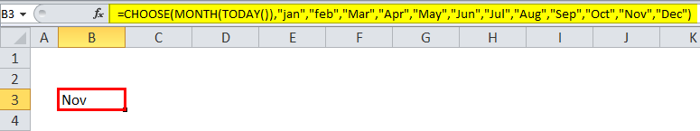
Using Choose & Today Function
Using the month function, we can use the choose & Today function to get the exact month name, wherein the above example shows we have used only the MONTH function to get the month value. In the below example, we have used the month function along with CHOOSE and TODAY.
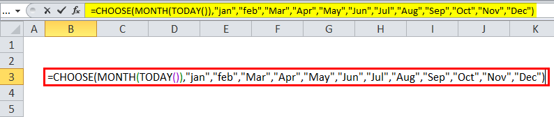
This dynamic formula will return the name of the month instead of the month number.
How to Use MONTH Function in Excel?
MONTH Function in excel is very simple easy to use. Let us now see how to use the MONTH Function in Excel with the help of some examples.
You can download this MONTH Function Excel Template here – MONTH Function Excel Template
Example #1
To find out today month, we can use the below formula:
=MONTH(TODAY())
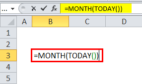
Which will return the current today month.
Let see to extract the month value with the below example
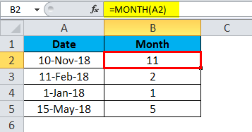
Example #2
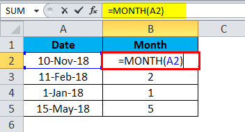
In the above example, we have retrieved the exact month by using the Month function to get the month name.
Example #3
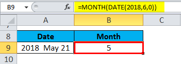
In certain scenarios, we can see Year, a month, and a day will be given. In this case, we cannot use the MONTH function. To get an accurate result, we can use the Month Function along with the date function.
Date Function:
Formula:
DATE( year, month, day )
where the year, month, and day arguments are integers representing the year, month, and day of the required date.
In the below example, we have used the Month Function and the date function to get the proper result.
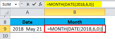
The Result will be:
Using the End of Month Function in Excel
If we need to find out the end of the month, EOMONTH can be useful to find out exactly.
To calculate the last day of a month based on a given date, you can use the EOMONTH function. Let’s see the below example works.
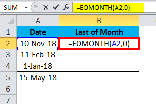
So in the above example, we can see A1 columns, which have a day, Month & Year, and B1 Columns, showing the Last day of the month using the EOMONTH function.
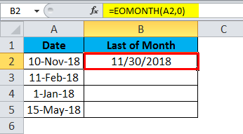
We can drag the formula by using Ctrl + D or double click on the right corner of the cell B2.
In this way, we can easily extract the end of the month without using a calendar.
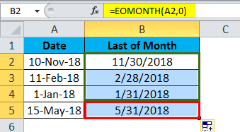
How EOMONTH Formula Works?
This EOMONTH Function allows you to get the last day of the month in the future or past month. If we use Zero(o) for months, EOMONTH will return the last day of the month in the same month, which we have seen in the above example. To get the last day of the prior month, we can use the below formula to execute:
Formula:
=EOMONTH(date,-1)
To get the last day of the next month, we can use the below formula to execute:
Formula:
=EOMONTH(date,1)
Alternatively, we can use the Date, Year and Month function to return the last day of the Month.
Formula:
=DATE(YEAR(date),MONTH(date)+1,0)
So in the above example, we can see various months in the A1 columns, and B1 shows the Last day of the month.
In this way, we can easily extract the end of the month without using a calendar.
Date Function Arguments
The excel date function is a built-in function in excel that will come under the Date/Time Function, where it returns the serial date value for a date.
A formula for DATE Function:
=DATE( year, month, day )
Arguments:
Year: A a number that is between 1 and 4 digits that represent the year.
Month: This represents month value; if the month value is greater than 12, then every 12 months will add1 one year to the year value.
Day: This represents day Value. If the day value is greater than the number of days, then the exact number of months will be added to the month value.
Example
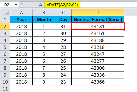
If we enter the date by default, excel will take as a general format which is shown below:
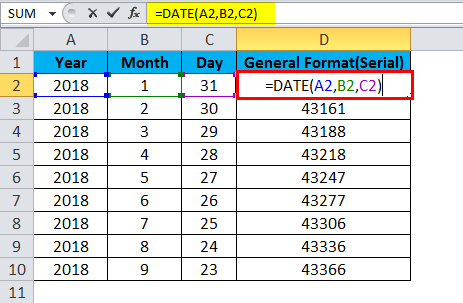
It will take as a general format which is shown below:
So in order to get the exact date to be displayed, we have to choose the format cells, and then we need to choose the day, month & year format.
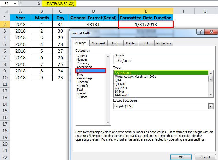
In the above example, we have formatted the cell to get the appropriate date, month & year.
Common Errors We will Face While Using Month Function in Excel:
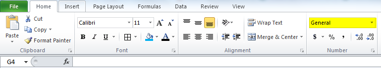
If we normally enter the date in the cell by default, excel will take an integer value because of “General format”.
So whenever we wish to update the date in the cell, we need to format the cell and choose the appropriate date, month and Year format.
Things to Remember
- The Date from which you want to get the month number should be a valid date.
- If you mention an invalid date, it will return #VALUE! error.
- if you skip entering any value in serial_number, it will return.
Recommended Articles
This has been a guide to MONTH in Excel. Here we discuss the MONTH Formula in Excel and how to use MONTH Function in Excel along with excel examples and downloadable excel templates. You may also look at these useful functions in excel –
- VBA Month
- Excel DATEDIF Function
- Excel Add Months to Dates
- WEEKDAY Formula in Excel
How to plus or minus exactly one month in Excel?
The best way is to use a built in function in the analysis toolpack, edate.
=edate([date], [months])
Date is the date you are calculating from. Months is how many months you want to add. If you want to go backwards, then months is a negative number. So, 1 months later, put 1; 4 months ago, put -4.
Unfortunately, as much as it seems intuitive, using the date function does not work as intended.
=date(year([date]), month([date])+1, day([date]))
The problem is if the month doesn’t have a certain day, the calculation gets extended into the next month. For example, the formula below returns March 2, 2011 instead of the intended February 28, 2011.
=date(year(DATE(2011,1,1)), month(DATE(2011,1,1))+1, day(DATE(2011,1,1)))
How to get the last day of the month in Excel?
Easiest way, once again, is to use a built in funciton in the analyst toolpack, eomonth.
=edate([date], [months])
The function takes the date provided and uses the second parameter to determine the number of months future or past that should be calculated. So, if you want the last day of the current month:
=edate(now(), 0)
Similar to above, to count backwards, negative numbers for months.
0 people found this article useful
0 people found this article useful
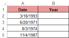
Excel spreadsheets provide the ability to work with various types of textual and numerical information. Date processing is also available. In this case, there may be a need to extract from the general meaning of a specific number, for example, a year. There are separate functions for this: YEAR, MONTH, DAY and DAY.
Examples of using functions for date processing in Excel
Excel tables store dates that are presented as a sequence of numeric values. It begins on January 1, 1900. This date will correspond to the number 1. At the same time, January 1, 2009 is laid down in the tables, as the number 39813. This is the number of days between the two designated dates.
The function YEAR is used similarly to the adjacent:
- MONTH;
- DAY;
- WEEKDAY.
All of them display numerical values corresponding to the Gregorian calendar. Even if in the Excel spreadsheet, the Hijra calendar was chosen to display the entered date, then when isolating the year and other composite values by functions, the application will present a number that is equivalent to the Gregorian system of chronology.
To use the YEAR function, you need to enter into the cell the following function formula with one argument:
=YEAR(cell address with date in numeric format)
The function argument is required. It can be replaced by «date_number_number». In the examples below, you can clearly see this. It is important to remember that when displaying the date as text (automatic orientation on the left edge of the cell), the YEAR function will not be executed. Its result will be the # SIGN. Therefore, formatted dates must be presented in a numerical version. Days, months and year can be separated by a dot, slash or comma.
Consider an example of working with the YEAR function in Excel. If we need to get a year from the original date, the function AVAILABLE will not help us since it does not work with dates, but only with text and numeric values. To separate the year, month or day from the full date for this, Excel provides functions for working with dates.
Example: There is a table with a list of dates and in each of them it is necessary to separate the value of only the year.
We introduce the original data in Excel.
To solve the problem, it is necessary to enter the formula in the cells of column B:
=YEAR(the address of the cell, from the date of which you need to isolate the year value)
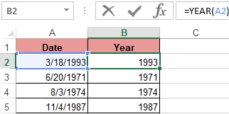
As a result, we extract years from each date.
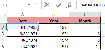
A similar example of the MONTH function in Excel:
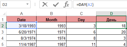
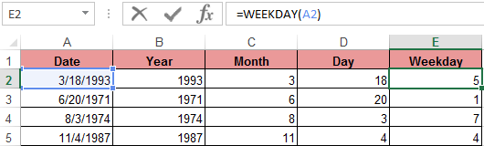
An example of working with functions DAY and WEEKDAY. The DAY function gets to calculate from the date the number of any day:
WEEKDAY function returns the number of the day of the week (1-Monday, 2-Tuesday …, etc.) for any date:
In the second optional argument of the WEEKDAY function, the number 2 may specified for our day of the week countdown format (Monday-1 through Sunday-7):
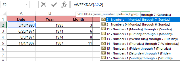
If you omit the second optional argument, then the default format will be used (English from Sunday-1 to Saturday-7).
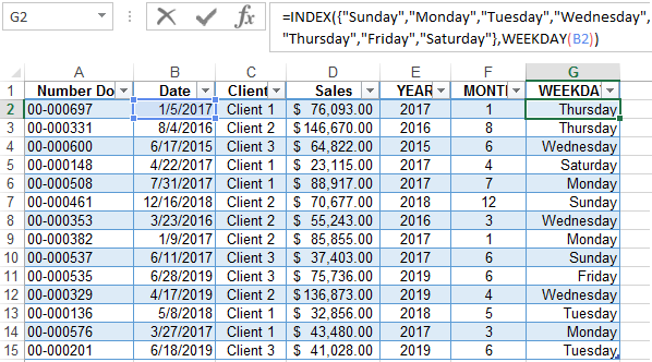
Create a formula of the combination of the functions INDEX and WEEKDAY:
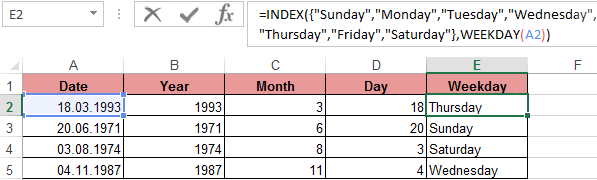
We obtain a more understandable form of the implementation of this function.
Examples of the practical use of functions for working with dates
These primitive functions are very useful when grouping data by: years, months, days of the week, and specific days.
Suppose we have a simple sales report:
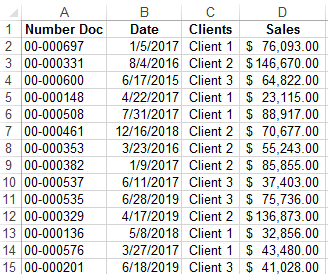
We need to quickly organize data for visual analysis without using pivot tables. To do this, we will bring the report into a table where it is convenient and quickly to group data by year, month and day of the week:
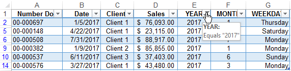
Now we have a tool to work with this sales report. We can filter and segment data by specific time criteria:
In addition, you can make a histogram to analyze the best-selling days of the week, to understand which day of the week has the largest number of sales:
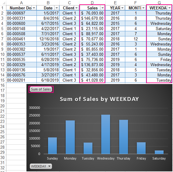
In this form, it is very convenient to segment sales reports for long, medium and short periods of time.
It should be immediately noted that in order to get the difference between the two dates, none of the above functions will help us. For this task, you should use a specially designed function DATEDIF:
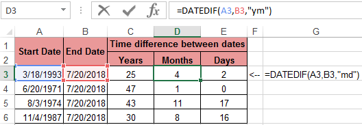
Download examples fo functions YEAR MONTH DAY WEEKDAY and DATEDIF
The type of values in the date cells requires a special approach to data processing. Therefore, you should use the appropriate type of function in Excel.