
If you’re new to Excel for the web, you’ll soon find that it’s more than just a grid in which you enter numbers in columns or rows. Yes, you can use Excel for the web to find totals for a column or row of numbers, but you can also calculate a mortgage payment, solve math or engineering problems, or find a best case scenario based on variable numbers that you plug in.
Excel for the web does this by using formulas in cells. A formula performs calculations or other actions on the data in your worksheet. A formula always starts with an equal sign (=), which can be followed by numbers, math operators (such as a plus or minus sign), and functions, which can really expand the power of a formula.
For example, the following formula multiplies 2 by 3 and then adds 5 to that result to come up with the answer, 11.
=2*3+5
This next formula uses the PMT function to calculate a mortgage payment ($1,073.64), which is based on a 5 percent interest rate (5% divided by 12 months equals the monthly interest rate) over a 30-year period (360 months) for a $200,000 loan:
=PMT(0.05/12,360,200000)
Here are some additional examples of formulas that you can enter in a worksheet.
-
=A1+A2+A3 Adds the values in cells A1, A2, and A3.
-
=SQRT(A1) Uses the SQRT function to return the square root of the value in A1.
-
=TODAY() Returns the current date.
-
=UPPER(«hello») Converts the text «hello» to «HELLO» by using the UPPER worksheet function.
-
=IF(A1>0) Tests the cell A1 to determine if it contains a value greater than 0.
The parts of a formula
A formula can also contain any or all of the following: functions, references, operators, and constants.

1. Functions: The PI() function returns the value of pi: 3.142…
2. References: A2 returns the value in cell A2.
3. Constants: Numbers or text values entered directly into a formula, such as 2.
4. Operators: The ^ (caret) operator raises a number to a power, and the * (asterisk) operator multiplies numbers.
Using constants in formulas
A constant is a value that is not calculated; it always stays the same. For example, the date 10/9/2008, the number 210, and the text «Quarterly Earnings» are all constants. An expression or a value resulting from an expression is not a constant. If you use constants in a formula instead of references to cells (for example, =30+70+110), the result changes only if you modify the formula.
Using calculation operators in formulas
Operators specify the type of calculation that you want to perform on the elements of a formula. There is a default order in which calculations occur (this follows general mathematical rules), but you can change this order by using parentheses.
Types of operators
There are four different types of calculation operators: arithmetic, comparison, text concatenation, and reference.
Arithmetic operators
To perform basic mathematical operations, such as addition, subtraction, multiplication, or division; combine numbers; and produce numeric results, use the following arithmetic operators.
|
Arithmetic operator |
Meaning |
Example |
|
+ (plus sign) |
Addition |
3+3 |
|
– (minus sign) |
Subtraction |
3–1 |
|
* (asterisk) |
Multiplication |
3*3 |
|
/ (forward slash) |
Division |
3/3 |
|
% (percent sign) |
Percent |
20% |
|
^ (caret) |
Exponentiation |
3^2 |
Comparison operators
You can compare two values with the following operators. When two values are compared by using these operators, the result is a logical value — either TRUE or FALSE.
|
Comparison operator |
Meaning |
Example |
|
= (equal sign) |
Equal to |
A1=B1 |
|
> (greater than sign) |
Greater than |
A1>B1 |
|
< (less than sign) |
Less than |
A1<B1 |
|
>= (greater than or equal to sign) |
Greater than or equal to |
A1>=B1 |
|
<= (less than or equal to sign) |
Less than or equal to |
A1<=B1 |
|
<> (not equal to sign) |
Not equal to |
A1<>B1 |
Text concatenation operator
Use the ampersand (&) to concatenate (join) one or more text strings to produce a single piece of text.
|
Text operator |
Meaning |
Example |
|
& (ampersand) |
Connects, or concatenates, two values to produce one continuous text value |
«North»&»wind» results in «Northwind» |
Reference operators
Combine ranges of cells for calculations with the following operators.
|
Reference operator |
Meaning |
Example |
|
: (colon) |
Range operator, which produces one reference to all the cells between two references, including the two references. |
B5:B15 |
|
, (comma) |
Union operator, which combines multiple references into one reference |
SUM(B5:B15,D5:D15) |
|
(space) |
Intersection operator, which produces one reference to cells common to the two references |
B7:D7 C6:C8 |
The order in which Excel for the web performs operations in formulas
In some cases, the order in which a calculation is performed can affect the return value of the formula, so it’s important to understand how the order is determined and how you can change the order to obtain the results you want.
Calculation order
Formulas calculate values in a specific order. A formula always begins with an equal sign (=). Excel for the web interprets the characters that follow the equal sign as a formula. Following the equal sign are the elements to be calculated (the operands), such as constants or cell references. These are separated by calculation operators. Excel for the web calculates the formula from left to right, according to a specific order for each operator in the formula.
Operator precedence
If you combine several operators in a single formula, Excel for the web performs the operations in the order shown in the following table. If a formula contains operators with the same precedence—for example, if a formula contains both a multiplication and division operator— Excel for the web evaluates the operators from left to right.
|
Operator |
Description |
|
: (colon) (single space) , (comma) |
Reference operators |
|
– |
Negation (as in –1) |
|
% |
Percent |
|
^ |
Exponentiation |
|
* and / |
Multiplication and division |
|
+ and – |
Addition and subtraction |
|
& |
Connects two strings of text (concatenation) |
|
= |
Comparison |
Use of parentheses
To change the order of evaluation, enclose in parentheses the part of the formula to be calculated first. For example, the following formula produces 11 because Excel for the web performs multiplication before addition. The formula multiplies 2 by 3 and then adds 5 to the result.
=5+2*3
In contrast, if you use parentheses to change the syntax, Excel for the web adds 5 and 2 together and then multiplies the result by 3 to produce 21.
=(5+2)*3
In the following example, the parentheses that enclose the first part of the formula force Excel for the web to calculate B4+25 first and then divide the result by the sum of the values in cells D5, E5, and F5.
=(B4+25)/SUM(D5:F5)
Using functions and nested functions in formulas
Functions are predefined formulas that perform calculations by using specific values, called arguments, in a particular order, or structure. Functions can be used to perform simple or complex calculations.
The syntax of functions
The following example of the ROUND function rounding off a number in cell A10 illustrates the syntax of a function.
1. Structure. The structure of a function begins with an equal sign (=), followed by the function name, an opening parenthesis, the arguments for the function separated by commas, and a closing parenthesis.
2. Function name. For a list of available functions, click a cell and press SHIFT+F3.
3. Arguments. Arguments can be numbers, text, logical values such as TRUE or FALSE, arrays, error values such as #N/A, or cell references. The argument you designate must produce a valid value for that argument. Arguments can also be constants, formulas, or other functions.
4. Argument tooltip. A tooltip with the syntax and arguments appears as you type the function. For example, type =ROUND( and the tooltip appears. Tooltips appear only for built-in functions.
Entering functions
When you create a formula that contains a function, you can use the Insert Function dialog box to help you enter worksheet functions. As you enter a function into the formula, the Insert Function dialog box displays the name of the function, each of its arguments, a description of the function and each argument, the current result of the function, and the current result of the entire formula.
To make it easier to create and edit formulas and minimize typing and syntax errors, use Formula AutoComplete. After you type an = (equal sign) and beginning letters or a display trigger, Excel for the web displays, below the cell, a dynamic drop-down list of valid functions, arguments, and names that match the letters or trigger. You can then insert an item from the drop-down list into the formula.
Nesting functions
In certain cases, you may need to use a function as one of the arguments of another function. For example, the following formula uses a nested AVERAGE function and compares the result with the value 50.
1. The AVERAGE and SUM functions are nested within the IF function.
Valid returns When a nested function is used as an argument, the nested function must return the same type of value that the argument uses. For example, if the argument returns a TRUE or FALSE value, the nested function must return a TRUE or FALSE value. If the function doesn’t, Excel for the web displays a #VALUE! error value.
Nesting level limits A formula can contain up to seven levels of nested functions. When one function (we’ll call this Function B) is used as an argument in another function (we’ll call this Function A), Function B acts as a second-level function. For example, the AVERAGE function and the SUM function are both second-level functions if they are used as arguments of the IF function. A function nested within the nested AVERAGE function is then a third-level function, and so on.
Using references in formulas
A reference identifies a cell or a range of cells on a worksheet, and tells Excel for the web where to look for the values or data you want to use in a formula. You can use references to use data contained in different parts of a worksheet in one formula or use the value from one cell in several formulas. You can also refer to cells on other sheets in the same workbook, and to other workbooks. References to cells in other workbooks are called links or external references.
The A1 reference style
The default reference style By default, Excel for the web uses the A1 reference style, which refers to columns with letters (A through XFD, for a total of 16,384 columns) and refers to rows with numbers (1 through 1,048,576). These letters and numbers are called row and column headings. To refer to a cell, enter the column letter followed by the row number. For example, B2 refers to the cell at the intersection of column B and row 2.
|
To refer to |
Use |
|
The cell in column A and row 10 |
A10 |
|
The range of cells in column A and rows 10 through 20 |
A10:A20 |
|
The range of cells in row 15 and columns B through E |
B15:E15 |
|
All cells in row 5 |
5:5 |
|
All cells in rows 5 through 10 |
5:10 |
|
All cells in column H |
H:H |
|
All cells in columns H through J |
H:J |
|
The range of cells in columns A through E and rows 10 through 20 |
A10:E20 |
Making a reference to another worksheet In the following example, the AVERAGE worksheet function calculates the average value for the range B1:B10 on the worksheet named Marketing in the same workbook.

1. Refers to the worksheet named Marketing
2. Refers to the range of cells between B1 and B10, inclusively
3. Separates the worksheet reference from the cell range reference
The difference between absolute, relative and mixed references
Relative references A relative cell reference in a formula, such as A1, is based on the relative position of the cell that contains the formula and the cell the reference refers to. If the position of the cell that contains the formula changes, the reference is changed. If you copy or fill the formula across rows or down columns, the reference automatically adjusts. By default, new formulas use relative references. For example, if you copy or fill a relative reference in cell B2 to cell B3, it automatically adjusts from =A1 to =A2.

Absolute references An absolute cell reference in a formula, such as $A$1, always refer to a cell in a specific location. If the position of the cell that contains the formula changes, the absolute reference remains the same. If you copy or fill the formula across rows or down columns, the absolute reference does not adjust. By default, new formulas use relative references, so you may need to switch them to absolute references. For example, if you copy or fill an absolute reference in cell B2 to cell B3, it stays the same in both cells: =$A$1.

Mixed references A mixed reference has either an absolute column and relative row, or absolute row and relative column. An absolute column reference takes the form $A1, $B1, and so on. An absolute row reference takes the form A$1, B$1, and so on. If the position of the cell that contains the formula changes, the relative reference is changed, and the absolute reference does not change. If you copy or fill the formula across rows or down columns, the relative reference automatically adjusts, and the absolute reference does not adjust. For example, if you copy or fill a mixed reference from cell A2 to B3, it adjusts from =A$1 to =B$1.

The 3-D reference style
Conveniently referencing multiple worksheets If you want to analyze data in the same cell or range of cells on multiple worksheets within a workbook, use a 3-D reference. A 3-D reference includes the cell or range reference, preceded by a range of worksheet names. Excel for the web uses any worksheets stored between the starting and ending names of the reference. For example, =SUM(Sheet2:Sheet13!B5) adds all the values contained in cell B5 on all the worksheets between and including Sheet 2 and Sheet 13.
-
You can use 3-D references to refer to cells on other sheets, to define names, and to create formulas by using the following functions: SUM, AVERAGE, AVERAGEA, COUNT, COUNTA, MAX, MAXA, MIN, MINA, PRODUCT, STDEV.P, STDEV.S, STDEVA, STDEVPA, VAR.P, VAR.S, VARA, and VARPA.
-
3-D references cannot be used in array formulas.
-
3-D references cannot be used with the intersection operator (a single space) or in formulas that use implicit intersection.
What occurs when you move, copy, insert, or delete worksheets The following examples explain what happens when you move, copy, insert, or delete worksheets that are included in a 3-D reference. The examples use the formula =SUM(Sheet2:Sheet6!A2:A5) to add cells A2 through A5 on worksheets 2 through 6.
-
Insert or copy If you insert or copy sheets between Sheet2 and Sheet6 (the endpoints in this example), Excel for the web includes all values in cells A2 through A5 from the added sheets in the calculations.
-
Delete If you delete sheets between Sheet2 and Sheet6, Excel for the web removes their values from the calculation.
-
Move If you move sheets from between Sheet2 and Sheet6 to a location outside the referenced sheet range, Excel for the web removes their values from the calculation.
-
Move an endpoint If you move Sheet2 or Sheet6 to another location in the same workbook, Excel for the web adjusts the calculation to accommodate the new range of sheets between them.
-
Delete an endpoint If you delete Sheet2 or Sheet6, Excel for the web adjusts the calculation to accommodate the range of sheets between them.
The R1C1 reference style
You can also use a reference style where both the rows and the columns on the worksheet are numbered. The R1C1 reference style is useful for computing row and column positions in macros. In the R1C1 style, Excel for the web indicates the location of a cell with an «R» followed by a row number and a «C» followed by a column number.
|
Reference |
Meaning |
|
R[-2]C |
A relative reference to the cell two rows up and in the same column |
|
R[2]C[2] |
A relative reference to the cell two rows down and two columns to the right |
|
R2C2 |
An absolute reference to the cell in the second row and in the second column |
|
R[-1] |
A relative reference to the entire row above the active cell |
|
R |
An absolute reference to the current row |
When you record a macro, Excel for the web records some commands by using the R1C1 reference style. For example, if you record a command, such as clicking the AutoSum button to insert a formula that adds a range of cells, Excel for the web records the formula by using R1C1 style, not A1 style, references.
Using names in formulas
You can create defined names to represent cells, ranges of cells, formulas, constants, or Excel for the web tables. A name is a meaningful shorthand that makes it easier to understand the purpose of a cell reference, constant, formula, or table, each of which may be difficult to comprehend at first glance. The following information shows common examples of names and how using them in formulas can improve clarity and make formulas easier to understand.
|
Example Type |
Example, using ranges instead of names |
Example, using names |
|
Reference |
=SUM(A16:A20) |
=SUM(Sales) |
|
Constant |
=PRODUCT(A12,9.5%) |
=PRODUCT(Price,KCTaxRate) |
|
Formula |
=TEXT(VLOOKUP(MAX(A16,A20),A16:B20,2,FALSE),»m/dd/yyyy») |
=TEXT(VLOOKUP(MAX(Sales),SalesInfo,2,FALSE),»m/dd/yyyy») |
|
Table |
A22:B25 |
=PRODUCT(Price,Table1[@Tax Rate]) |
Types of names
There are several types of names that you can create and use.
Defined name A name that represents a cell, range of cells, formula, or constant value. You can create your own defined name. Also, Excel for the web sometimes creates a defined name for you, such as when you set a print area.
Table name A name for an Excel for the web table, which is a collection of data about a particular subject that is stored in records (rows) and fields (columns). Excel for the web creates a default Excel for the web table name of «Table1», «Table2», and so on, each time you insert an Excel for the web table, but you can change these names to make them more meaningful.
Creating and entering names
You create a name by using Create a name from selection. You can conveniently create names from existing row and column labels by using a selection of cells in the worksheet.
Note: By default, names use absolute cell references.
You can enter a name by:
-
Typing Typing the name, for example, as an argument to a formula.
-
Using Formula AutoComplete Use the Formula AutoComplete drop-down list, where valid names are automatically listed for you.
Using array formulas and array constants
Excel for the web doesn’t support creating array formulas. You can view the results of array formulas created in Excel desktop application, but you can’t edit or recalculate them. If you have the Excel desktop application, click Open in Excel to work with arrays.
The following array example calculates the total value of an array of stock prices and shares, without using a row of cells to calculate and display the individual values for each stock.
When you enter the formula ={SUM(B2:D2*B3:D3)} as an array formula, it multiples the Shares and Price for each stock, and then adds the results of those calculations together.
To calculate multiple results Some worksheet functions return arrays of values, or require an array of values as an argument. To calculate multiple results with an array formula, you must enter the array into a range of cells that has the same number of rows and columns as the array arguments.
For example, given a series of three sales figures (in column B) for a series of three months (in column A), the TREND function determines the straight-line values for the sales figures. To display all the results of the formula, it is entered into three cells in column C (C1:C3).
When you enter the formula =TREND(B1:B3,A1:A3) as an array formula, it produces three separate results (22196, 17079, and 11962), based on the three sales figures and the three months.
Using array constants
In an ordinary formula, you can enter a reference to a cell containing a value, or the value itself, also called a constant. Similarly, in an array formula you can enter a reference to an array, or enter the array of values contained within the cells, also called an array constant. Array formulas accept constants in the same way that non-array formulas do, but you must enter the array constants in a certain format.
Array constants can contain numbers, text, logical values such as TRUE or FALSE, or error values such as #N/A. Different types of values can be in the same array constant — for example, {1,3,4;TRUE,FALSE,TRUE}. Numbers in array constants can be in integer, decimal, or scientific format. Text must be enclosed in double quotation marks — for example, «Tuesday».
Array constants cannot contain cell references, columns or rows of unequal length, formulas, or the special characters $ (dollar sign), parentheses, or % (percent sign).
When you format array constants, make sure you:
-
Enclose them in braces ( { } ).
-
Separate values in different columns by using commas (,). For example, to represent the values 10, 20, 30, and 40, you enter {10,20,30,40}. This array constant is known as a 1-by-4 array and is equivalent to a 1-row-by-4-column reference.
-
Separate values in different rows by using semicolons (;). For example, to represent the values 10, 20, 30, and 40 in one row and 50, 60, 70, and 80 in the row immediately below, you enter a 2-by-4 array constant: {10,20,30,40;50,60,70,80}.
Ready solutions for Excel with the help of formulas working with data spans in the process of complex computations and calculations.
Computing operations with the help of formulas
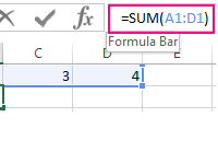 The Formula Bar in Excel, its settings and the purpose.
How to use the formula string and what advantages does it provide for entering and editing data in cells? How to enable or disable the formula bar in the program settings.
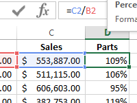 Percentage of the plan implementation by formula in Excel.
The examples of two formulas for calculating of percentages from numbers when analyzing the implementation of sales plans. The example, when and how to use the percentage format of cells.
Excel formulas allow you to identify relationships between values in your spreadsheet’s cells, perform mathematical calculations with those values, and return the resulting value in the cell of your choice. Sum, subtraction, percentage, division, average, and even dates/times are among the formulas that can be performed automatically. For example, =A1+A2+A3+A4+A5, which finds the sum of the range of values from cell A1 to cell A5.
Excel Functions: A formula is a mathematical expression that computes the value of a cell. Functions are predefined formulas that are already in Excel. Functions carry out specific calculations in a specific order based on the values specified as arguments or parameters. For example, =SUM (A1:A10). This function adds up all the values in cells A1 through A10.
How to Insert Formulas in Excel?
This horizontal menu, shown below, in more recent versions of Excel allows you to find and insert Excel formulas into specific cells of your spreadsheet. On the Formulas tab, you can find all available Excel functions in the Function Library:
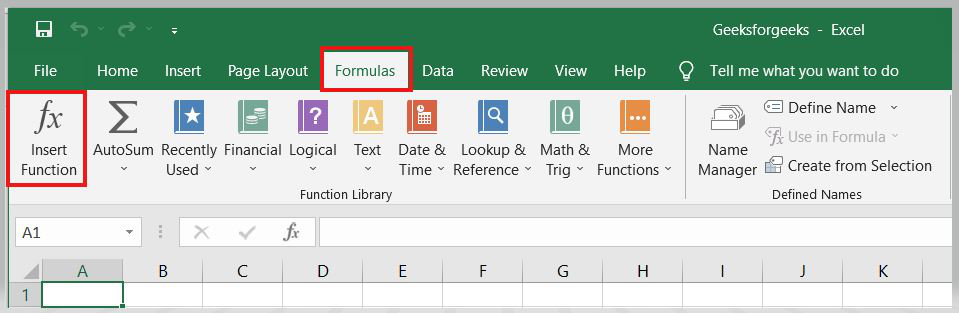
The more you use Excel formulas, the easier it will be to remember and perform them manually. Excel has over 400 functions, and the number is increasing from version to version. The formulas can be inserted into Excel using the following method:
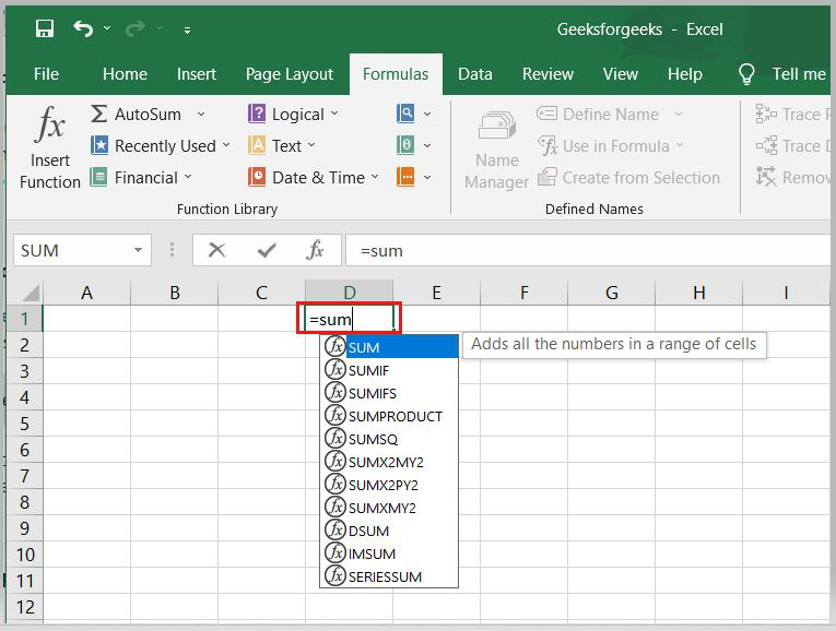
1. Simple insertion of the formula(Typing a formula in the cell):
Typing a formula into a cell or the formula bar is the simplest way to insert basic Excel formulas. Typically, the process begins with typing an equal sign followed by the name of an Excel function. Excel is quite intelligent in that it displays a pop-up function hint when you begin typing the name of the function.
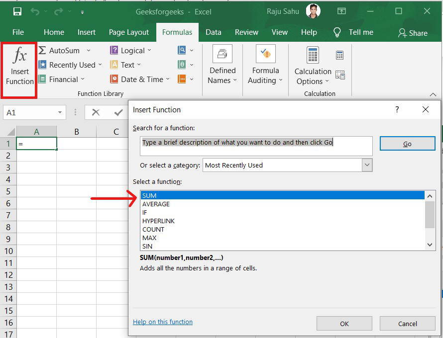
2. Using the Insert Function option on the Formulas Tab:
If you want complete control over your function insertion, use the Excel Insert Function dialogue box. To do so, go to the Formulas tab and select the first menu, Insert Function. All the functions will be available in the dialogue box.
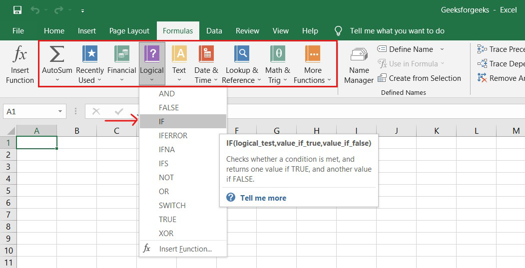
3. Choosing a Formula from One of the Formula Groups in the Formula Tab:
This option is for those who want to quickly dive into their favorite functions. Navigate to the Formulas tab and select your preferred group to access this menu. Click to reveal a sub-menu containing a list of functions. You can then choose your preference. If your preferred group isn’t on the tab, click the More Functions option — it’s most likely hidden there.
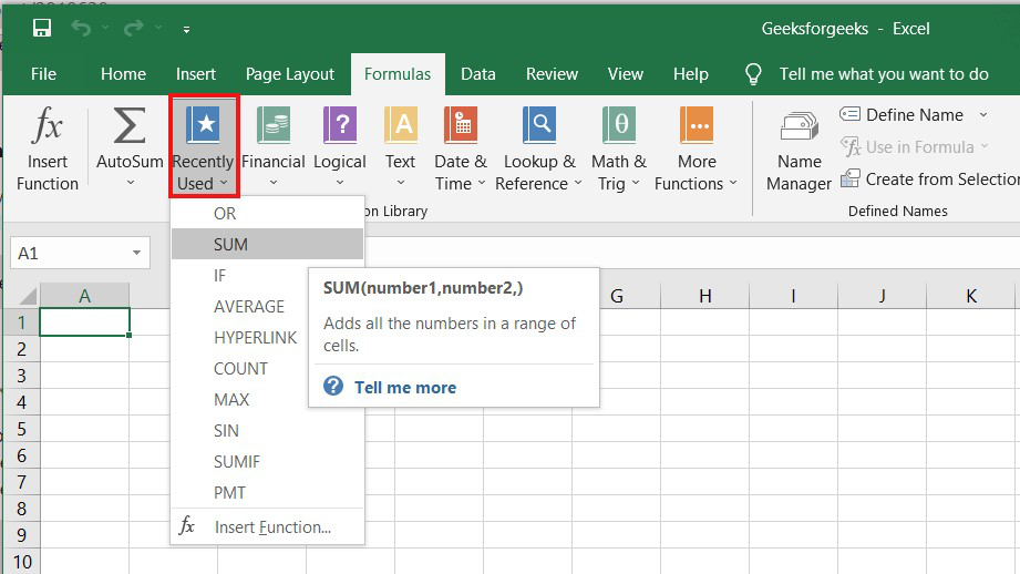
4. Use Recently Used Tabs for Quick Insertion:
If retyping your most recent formula becomes tedious, use the Recently Used menu. It’s on the Formulas tab, the third menu option after AutoSum.
Basic Excel Formulas and Functions:
1. SUM:
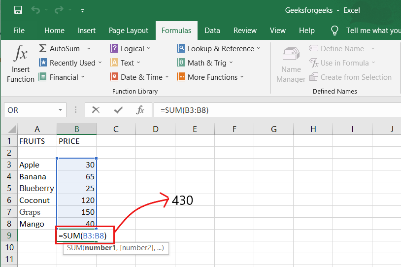
The SUM formula in Excel is one of the most fundamental formulas you can use in a spreadsheet, allowing you to calculate the sum (or total) of two or more values. To use the SUM formula, enter the values you want to add together in the following format: =SUM(value 1, value 2,…..).
Example: In the below example to calculate the sum of price of all the fruits, in B9 cell type =SUM(B3:B8). this will calculate the sum of B3, B4, B5, B6, B7, B8 Press “Enter,” and the cell will produce the sum: 430.
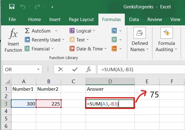
2. SUBTRACTION:
To use the subtraction formula in Excel, enter the cells you want to subtract in the format =SUM (A1, -B1). This will subtract a cell from the SUM formula by appending a negative sign before the cell being subtracted.
For example, if A3 was 300 and B3 was 225, =SUM(A1, -B1) would perform 300 + -225, returning a value of 75 in D3 cell.
3. MULTIPLICATION:
In Excel, enter the cells to be multiplied in the format =A3*B3 to perform the multiplication formula. An asterisk is used in this formula to multiply cell A3 by cell B3.
For example, if A3 was 300 and B3 was 225, =A1*B1 would return a value of 67500.
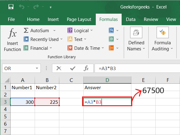
Highlight an empty cell in an Excel spreadsheet to multiply two or more values. Then, in the format =A1*B1…, enter the values or cells you want to multiply together. The asterisk effectively multiplies each value in the formula.
To return your desired product, press Enter. Take a look at the screenshot above to see how this looks.
4. DIVISION:
To use the division formula in Excel, enter the dividing cells in the format =A3/B3. This formula divides cell A3 by cell B3 with a forward slash, “/.”
For example, if A3 was 300 and B3 was 225, =A3/B3 would return a decimal value of 1.333333333.
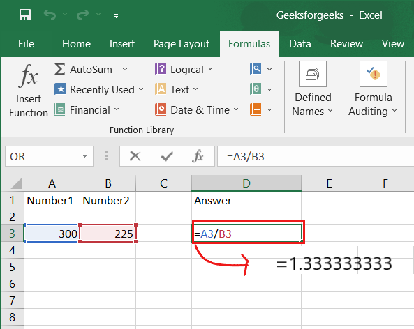
Division in Excel is one of the most basic functions available. To do so, highlight an empty cell, enter an equals sign, “=,” and then the two (or more) values you want to divide, separated by a forward slash, “/.” The output should look like this: =A3/B3, as shown in the screenshot above.
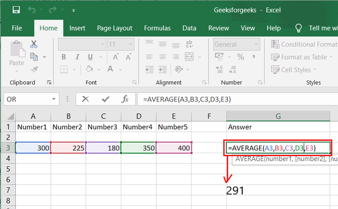
5. AVERAGE:
The AVERAGE function finds an average or arithmetic mean of numbers. to find the average of the numbers type = AVERAGE(A3.B3,C3….) and press ‘Enter’ it will produce average of the numbers in the cell.
For example, if A3 was 300, B3 was 225, C3 was 180, D3 was 350, E3 is 400 then =AVERAGE(A3,B3,C3,D3,E3) will produce 291.
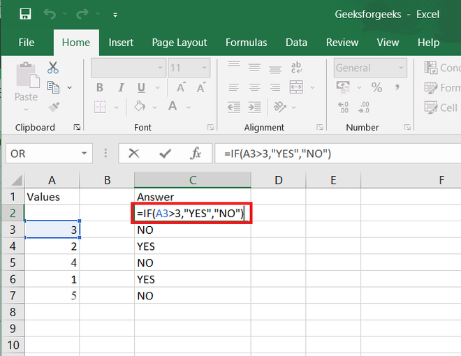
6. IF formula:
In Excel, the IF formula is denoted as =IF(logical test, value if true, value if false). This lets you enter a text value into a cell “if” something else in your spreadsheet is true or false.
For example, You may need to know which values in column A are greater than three. Using the =IF formula, you can quickly have Excel auto-populate a “yes” for each cell with a value greater than 3 and a “no” for each cell with a value less than 3.
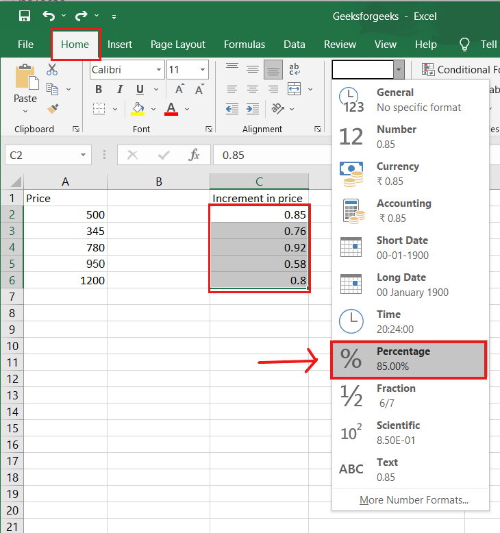
7. PERCENTAGE:
To use the percentage formula in Excel, enter the cells you want to calculate the percentage for in the format =A1/B1. To convert the decimal value to a percentage, select the cell, click the Home tab, and then select “Percentage” from the numbers dropdown.
There isn’t a specific Excel “formula” for percentages, but Excel makes it simple to convert the value of any cell into a percentage so you don’t have to calculate and reenter the numbers yourself.
The basic setting for converting a cell’s value to a percentage is found on the Home tab of Excel. Select this tab, highlight the cell(s) you want to convert to a percentage, and then select Conditional Formatting from the dropdown menu (this menu button might say “General” at first). Then, from the list of options that appears, choose “Percentage.” This will convert the value of each highlighted cell into a percentage. This feature can be found further down.
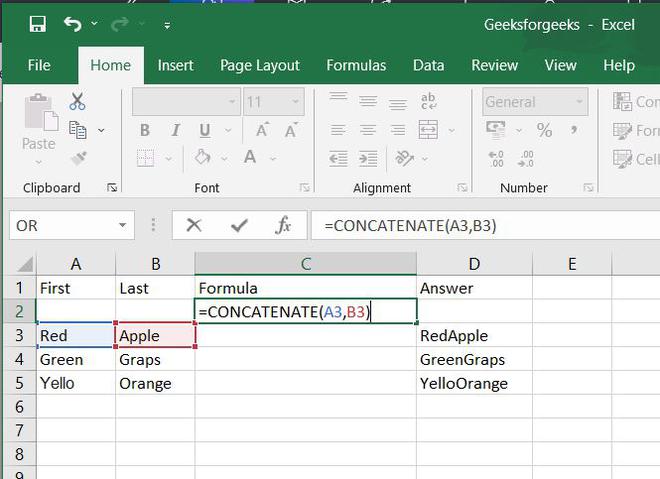
8. CONCATENATE:
CONCATENATE is a useful formula that combines values from multiple cells into the same cell.
For example , =CONCATENATE(A3,B3) will combine Red and Apple to produce RedApple.
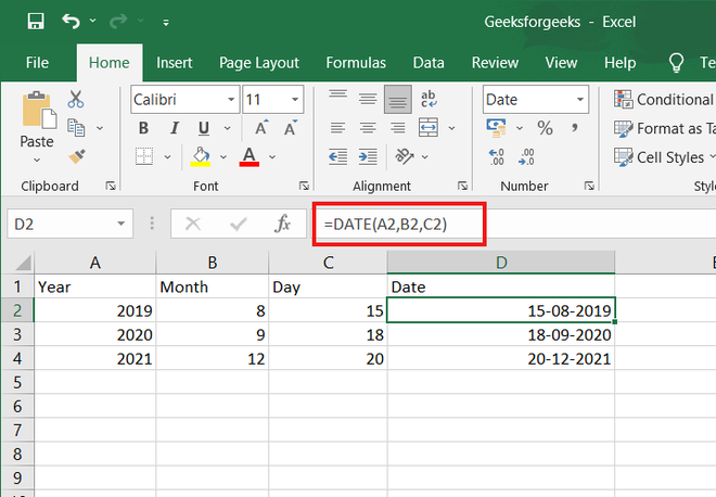
9. DATE:
DATE is the Excel DATE formula =DATE(year, month, day). This formula will return a date corresponding to the values entered in the parentheses, including values referred to from other cells.. For example, if A2 was 2019, B2 was 8, and C1 was 15, =DATE(A1,B1,C1) would return 15-08-2019.
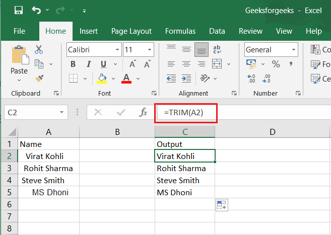
10. TRIM:
The TRIM formula in Excel is denoted =TRIM(text). This formula will remove any spaces that have been entered before and after the text in the cell. For example, if A2 includes the name ” Virat Kohli” with unwanted spaces before the first name, =TRIM(A2) would return “Virat Kohli” with no spaces in a new cell.
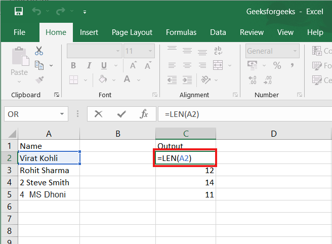
11. LEN:
LEN is the function to count the number of characters in a specific cell when you want to know the number of characters in that cell. =LEN(text) is the formula for this. Please keep in mind that the LEN function in Excel counts all characters, including spaces:
For example,=LEN(A2), returns the total length of the character in cell A2 including spaces.
Formulas
A formula in Excel is used to do mathematical calculations. Formulas always start with the equal sign (=) typed in the cell, followed by your calculation.
Formulas can be used for calculations such as:
=1+1=2*2=4/2=2
It can also be used to calculate values using cells as input.
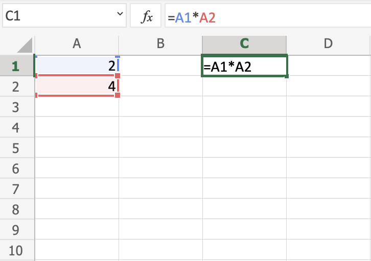
Let’s have a look at an example.
Type or copy the following values:
Now we want to do a calculation with those values.
Step by step:
- Select
C1and type (=) - Right click
A1 - Type (
+) - Right click
A2 - Press enter
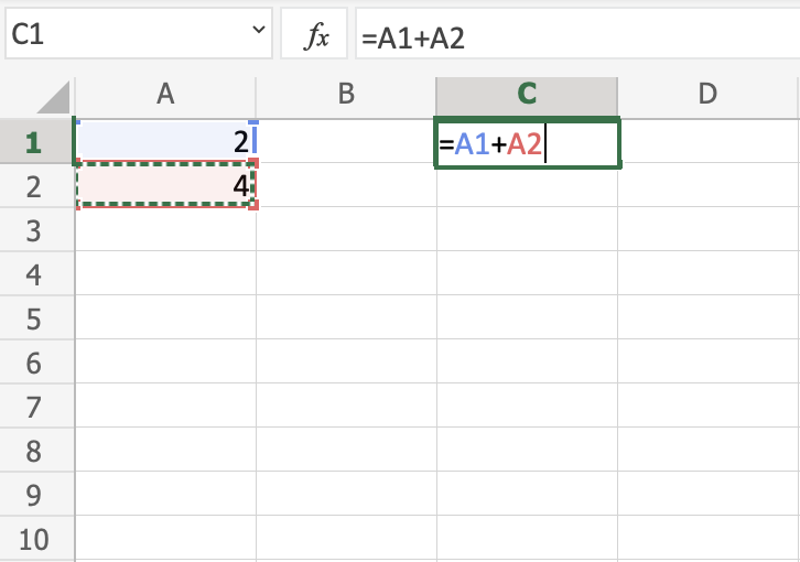
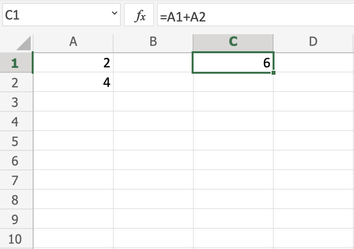
You got it! You have successfully calculated A1(2) + A2(4) = C1(6).
Note: Using cells to make calculations is an important part of Excel and you will use this alot as you learn.
Lets change from addition to multiplication, by replacing the (+) with a (*). It should now be =A1*A2, press enter to see what happens.
You got C1(8), right? Well done!
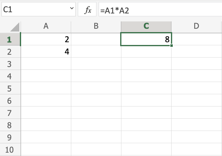
Excel is great in this way. It allows you to add values to cells and make you do calculations on them.
Now, try to change the multiplication (*) to subtraction (-) and dividing (/).
Delete all values in the sheet after you have tried the different combinations.
Let’s add new data for the next example, where we will help the Pokemon trainers to count their Pokeballs.
Type or copy the following values:
The data explained:
- Column
A: Pokemon Trainers - Row
1: Types of Pokeballs - Range
B2:D4: Amount of Pokeballs, Great balls and Ultra balls
Note: It is important to practice reading data to understand its context. In this example you should focus on the trainers and their Pokeballs, which have three different types: Pokeball, Great ball and Ultra ball.
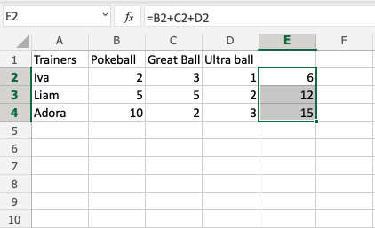
Let’s help Iva to count her Pokeballs. You find Iva in A2(Iva). The values in row 2 B2(2), C2(3), D2(1) belong to her.
Count the Pokeballs, step by step:
- Select cell
E2and type (=) - Right click
B2 - Type (
+) - Right click
C2 - Type (
+) - Right click
D2 - Hit enter
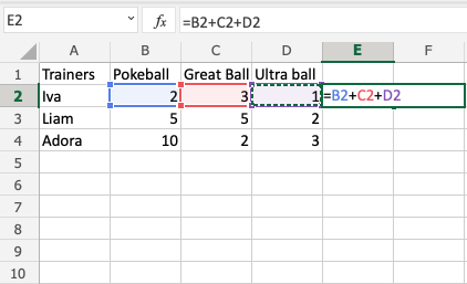
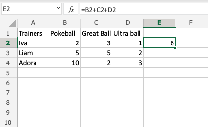
Did you get the value E2(6)? Good job! You have helped Iva to count her Pokeballs.
Now, let’s help Liam and Adora with counting theirs.
Do you remember the fill function that we learned about earlier? It can be used to continue calculations sidewards, downwards and upwards. Let’s try it!
Lets use the fill function to continue the formula, step by step:
- Select
E2 - Fill
E2:E4
That is cool, right? The fill function continued the calculation that you used for Iva and was able to understand that you wanted to count the cells in the next rows as well.
Now we have counted the Pokeballs for all three; Iva(6), Liam(12) and Adora(15).
Let’s see how many Pokeballs Iva, Liam and Adora have in total.
The total is called SUM in Excel.
There are two ways to calculate the SUM.
- Adding cells
- SUM function
Excel has many pre-made functions available for you to use. The SUM
function is one of the most used ones. You will learn more about functions in a later chapter.
Let’s try both approaches.
Note: You can navigate to the cells with your keyboard arrows instead of right clicking them. Try it!
Sum by adding cells, step by step:
- Select cell E5, and type
= - Left click
E2 - Type (
+) - Left click
E3 - Type (
+) - Left click
E4 - Hit enter

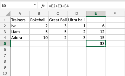
The result is E5(33).
Let’s try the SUM function.
Remember to delete the values that you currently have in E5.
SUM function, step by step:
- Type
E5(=) - Write SUM
- Double click SUM in the menu
- Mark the range
E2:E4 - Hit enter
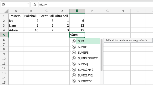
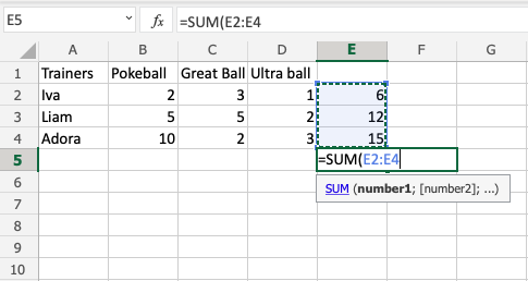

Great job! You have successfully calculated the SUM using the SUM function.
Iva, Liam and Adora have 33 Pokeballs in total.
Let’s change a value to see what happens. Type B2(7):

The value in cell B2 was changed from 2 to 7. Notice that the formulas are doing calculations when we change the value in the cells, and the SUM is updated from 33 to 38. It allows us to change values that are used by the formulas, and the calculations remain.
Chapter Summary
Values used in formulas can be typed directly and by using cells. The formula updates the result if you change the value of cells, which is used in the formula. The fill function can be used to continue your formulas upwards, downwards and sidewards. Excel has pre-built functions, such as SUM.
In the next chapter you will learn about relative and absolute references.
Test Yourself With Exercises
You may be familiar with Microsoft Excel. This application made by Microsoft Corporation is the application with the most users in the world in 140+ countries. This application has a myriad of Excel formulas that can accurately present numbers and data.
The primary function of Microsoft Excel is calculation, which is why it has been used by many users, both students and office workers. Despite other spreadsheet programs (competitors), Excel maintained its dominance and even became an industry standard.
Apparently, Excel seems too good to be true. All you have to do is enter an Excel formula, and almost everything you need to do manually can be done automatically. Use the best accounting software to do the cash flow forecast appropriately and analyze financial statements more optimally.
If you need to combine two sheets with the same data, Excel can do this. Do you need help with mathematics? Excel can do this. Are you using data from multiple cells? Excel can do this too.
In this article, you will understand the function of Excel in different professional fields. Then you’ll understand what formulas you need to know. Later, you will be able to apply automatic calculations to be used according to your needs.
Table Of Content
- The Uses of Excel in Professional Fields
- Complete Excel Formulas with Their Functions
- Conclusion
Also Read: 5 Common Bookkeeping Mistakes on Small Businesses
The Uses of Excel in Professional Fields
Many job openings require candidates to master Excel. Not surprisingly, excel is needed by a wide variety of fields of work that require data collection.
To that end, we will present the following professions, which can benefit from the use of Excel, among others:
Accountancy
It is widespread for accountants to be able to use Excel. The field of accounting benefits from using Microsoft Excel in several ways, including making it easier to calculate corporate profit and loss, identify large profits over a period, calculate employee salaries, and more.
An accountant can facilitate his work by using the accounting system as a tool he worked. The system can provide convenience in managing the company’s financial circulation and calculating it optimally and accurately.
Also Read: Salary Slip: Understanding, Benefits, Format, Example
Mathematical calculations
The next advantage of using Microsoft Excel is mathematical calculations. Use calculations to find data from numbers, subtractions, multiplications, and divisions, as well as various other variations such as calculating the slope.
Data processing
In data management, there are helpful excel formulas, including managing statistical databases, calculating data, searching for median values, and averages, and searching for the maximum and minimum values of data sets.
Graphic creation
Excel allows you to create graphics. Such as graphing population development data for one year, the graph of student library visits for one year, the student graduation graph for six years, the graph of student number development for three years, and others.
Table operations
The last application is to be able to operate the table. With a total of 1,084,576 rows and 16,384 columns in Microsoft Excel, it will make it easier for you to enter data that requires a large number of columns and rows.
Complete Excel Formulas with Their Functions
In addition to the functionality and use of Microsoft Excel mentioned earlier, operating this Excel program requires Excel formulas. Each formula has a different function that you can use for a specific need.
Here are the Excel formulas you need to know, among others:
| Formulas | Functional Description |
| SUM | Summing |
| AVERAGE | Looking for Average Values |
| AND | Finding Value by comparison and |
| NOT | Finding Value with Exceptions |
| OR | Finding Value by Comparison or |
| SINGLE IF | Looking for Values If Conditions ARE RIGHT/WRONG |
| MULTI IF | Finding Values If Conditions ARE RIGHT/WRONG With Many Comparisons |
| AREAS | View The Number of Areas (Range or Cells) |
| CHOOSE | View Selection Results Based on Index Numbers |
| HLOOKUP | Search for Data from a table organized in a horizontal format |
| VLOOKUP | Search for Data from a table arranged in an upright format |
| MATCH | Displays the position of a specific cell address |
| COUNTIF | Counting the Number of Cells in a Range with specific criteria |
| COUNTA | Counting the Number of Filled Cells |
| CEILING | Round the number up |
| FLOOR | Rounds numbers down |
| DAY | Looking for The Value of the Day |
| MONTH | Searching for the Value of the Moon |
| YEAR | Looking for Year Value |
| DATE | Get a Date Value |
| LOWER | Change text letters to lowercase |
| UPPER | Change Text Letters to UpperCase |
| PROPER | Change the Initial Character of the Text To UpperCase |
For more information about how to use the excel function formulas mentioned above, here is a detailed description, along with examples:
SUM
This Excel summation formula has the primary function of summing numbers in specific cells. However, it is also often used to complete a job or task quickly.
To use SUM, first create a summation table and enter the summation formula below. For example, =SUM(G8:H8), or as shown in the image below:
Then, if the SUM formula has been entered, press enters to specify the amount. As shown in the picture below:
AVERAGE
The primary function of the AVERAGE formula or the average formula in Excel is to find the average value of a variable. The trick is to create a table for grades and then enter the AVERAGE formula to determine the student’s grade point average. For example, =AVERAGE(D2:F2), as in the following image:
If you enter the AVERAGE formula, press enters to see the result, shown in the image below.
AND
The AND formula function generates a TRUE value if all previously tested arguments are correct or can return a FALSE value if all arguments or answers are incorrect.
To determine TRUE or FALSE, you must create a table and enter THE FORMULA AND. For example, =AND(G7>I7).
This technique is usually used to help fill out questionnaires or answer question columns to speed up the value-setting process.
NOT
The NOT formula has the opposite function of the AND formula because it produces TRUE if the condition tested is FALSE and FALSE if the condition tested is TRUE.
The first step is to create a table and enter the FORMULA NOT to find out the results. For example, as shown in the diagram below, =NOT(G7>J7).
OR
The OR is the following excel formula that will produce TRUE data if some given argument is correct. If all of the arguments presented are incorrect, the answer is FALSE.
A student’s average test score result is an example of how OR can use it in Excel. If it is less than 70, he must repeat the course; if it is greater than 70, the student graduates.
SINGLE IF
The IF function is to return a value that, when examined, is TRUE and another value that is visible as FALSE.
Not much different from the technique of using formulas in OR. It just seems more straightforward.
For example, when a student’s average grade is less than 75, that student does not graduate, and vice versa. How to create an IF formula is =IF(J8<75;” NOT GRADUATING”;” PASS”). To be clear, take a look at the following image:
After entering the formula, press enters, and the result will match what you ordered.
MULTI IF
This formula is a further lesson from SINGLE IF, but if SINGLE IF only uses only one condition with two options, The MULTI IF uses two terms and three options.
A Double/Multi FORMULA is a type of logic-IF formula consisting of 2 or more IF in formula writing. If a single IF only needs 1 IF, for example, =IF(B2=>=70;” Graduated”;” Failed”) then Double IF requires more than 1 IF, for example, =IF(B2>=70;” Good”;IF(B2>=50;” Enough”;” Less”)).
So that the full Excel formula will provide Syntax on Double / Multi IF, among others:
=IF(Logical_Test; Value_If_True;IF(Logical_Test; Value_If_True; Value_If_False))
AREAS
You can use the usability of AREAS if you want to calculate the number of areas you want to select. The AREAS formula can use the formula =AREAS(G6:K8).
The result is one area. The results are based on the example in the image of selecting only one range of cells.
CHOOSE
The primary function of a CHOOSE formula is to display selection results based on index numbers or sequences in reference (VALUE) that contain text, numeric, formula, or range names. The image below shows an example of how to write the CHOOSE formula.
Meanwhile, the results of the CHOOSE formula are shown in the image below.
HLOOKUP
The HLOOKUP function displays data from tables arranged horizontally. However, The arrangement of tables or data in the first row should be based on small to large sequences or raising them.
For example, the number 1,2,3,4… Or the letter A-Z. Sort by ascending the menu if you previously typed randomly. Cases like the ones listed below are examples.
=HLOOKUP(Cells that contain packet types; Range cell table details costs; The location of the data column you want to retrieve;0).
VLOOKUP
The primary function of the VLOOKUP formula is almost identical to the HLOOKUP formula; The difference is that the VLOOKUP formula displays data from tables arranged in an upright or vertical format. The requirement is that the first row of the data table is prepared in small to large order or up.
For example 1,2,3,4… Or the letter A-Z. For example 1,2,3,4… Or the letter A-Z. Sort through the Ascending menu if you previously typed randomly.
MATCH
The MATCH function is one of the components of an Excel formula that you can use to perform lookups or reference data searches.
The MATCH function works by finding the relative position of a value in a range or array and generating a number that is the index of the cell’s relative position that contains the value it is looking for.
The use of the Excel MATCH function must follow the syntax rules, namely MATCH(lookup_value, lookup_array, [match_type])
To better understand, understand the image below:
COUNTIF
COUNTIF is a helpful formula for counting the number of cells that have the same criteria. As a result, you no longer have to struggle with data sorting.
Assume you’re doing a survey. You want to know how many civil servants there are out of 20 respondents. As a result, you can use the following formulas:
To get started, all you need to do is enter the range of cells you want to identify into the COUNTIF formula (B2:B21)
Then, enter the cell calculation criteria, namely “PNS” (must be in quotation marks).
This formula produces a result of 7. So, out of 20 respondents, seven were civil servants.
COUNTA
COUNTA has the function of counting the number of cells that contain numbers and the number of cells that contain anything. As a result, you can determine the number of cells that are not empty.
Assume that cells A1 through D1 are words and cells G1 through I1 number. Therefore the use of the formula is =COUNTA(A1:I1)
That results in 7 because the empty cells are only E1 and F1.
CEILING
The CEILING formula can round the number UP at the multiple values of a specific number. The formula is CEILING (CELLS number; Multiples).
Misalnya, CEILING(G9;100). Then the number on Cells G9 will be rounded up with a multiple of 100.
FLOOR
If the previous use of the formula is to round to the nearest integer and above, the FLOOR formula is used to round to the nearest integer. The formula is almost identical to the one for CEILING, but with the addition of FLOOR.
The FLOOR formula is FLOOR (Number cell; Multiples).
DAY
The DAY formula is used to find the date type data’s day (in the numbers 1-31). Consider the DAY function (column B). The date data in column A will be extracted and converted into numbers 1-31, following the explanation through the image:
After entering the formula =DAY(NUMBER), press enters and see the results below:
MONTH
Almost similar to the DAY formula, the use of the MONTH formula to search for months (in numbers 1-12) from date type data. For example, the use of the MONTH function (column K) of a column I date data, after extracting it, produces the numbers 1-12 as in the figure below:
YEAR
Meanwhile, there is a YEAR formula. The way you use this formula is similar to the way the previous two formulas were. The use of the YEAR formula takes years (in the range of 1900-9999) from date-type data.
DATE
The DATE formula has a function that allows you to get date data types by entering years, months, and days. The DATE function is the opposite of the DAY, MONTH, and YEAR functions, which describe month and year-type data from their respective dates.
Year, month, and day data in the form of numbers combined with the DATE function generate data with data types, as shown in the figure below. Date formula writing image, namely:
LOWER
The lower formula function converts all uppercase letters in the text to lowercase. To use the formula, type the LOWER command, and texts will convert the desired writing to lowercase.
For example, when implementing the LOWER formula with the formula =LOWER (Don’t Forget to Use HashMicro Software), the result is “don’t forget to use has micro software.”
UPPER
In addition to lower formulas, Microsoft Excel includes upper formulas. The use of UPPER is to convert all text containing lowercase letters into uppercase, the opposite of the LOWER function.
For example, if you type UPPER (hashmicro), your writing will be entirely in capital letters.
PROPER
Sometimes you forget to write sentences in all lowercase letters and no capital letters. So with the PROPER formula, you can capitalize on the first character in each word while keeping the rest. The formula is APPROPRIATE (text).
Conclusion
Although understanding Excel entirely takes time, you will be familiar with all the correct formulas and applications.
In a company, the use of Excel is overwhelming, especially in presenting data, statistics, and company finances such as salaries. The digital world is bringing corporate transformation to provide information and payroll more easily with automated systems. You can use HashMicro accounting software as a tool to calculate financial circulation optimally and accurately.
Moreover, HashMicro has a system that helps with all your human resource and employee administration tasks. With HashMicro’s HRM Software, calculates salaries, and manages leave and attendance lists, reimbursement processes, timesheets, and other operational activities in just seconds.
Produce reports accurately and comprehensively like thousands of large companies that have joined HashMicro. To check out more, click here.
List of Basic Formulas and Functions
-
- SUM in Excel
- MAX Formula in Excel
- MIN Formula in Excel
- AVERAGE in Excel
- COUNT in Excel
- COUNTA in Excel
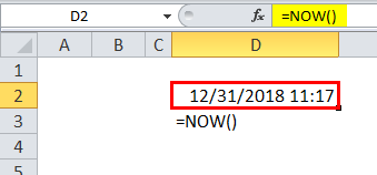
- NOW in Excel
- LEN in Excel
- ABS in Excel
- RAND in Excel
- RANDBETWEEN in Excel
- UPPER in Excel
- LOWER in Excel
- PROPER Function in Excel
What is Excel Formula?
Now, what do you mean by the Excel formula? It sounds like big jargon! But don’t worry! Excel formulas make life simple. You can use Excel formulas if you want to calculate numbers with a very dynamic passion. Excel formulas will calculate numbers or values for you so that you don’t have to spend much time calculating large numbers manually and risk making mistakes.
“A formula is an instruction given by the user to carry out some activity within spreadsheet, generally its calculation.”
This is the formal definition of an Excel formula. Our main concern is to learn basic Excel formulas in Excel so let’s look at How to enter a formula in Excel? When you enter an Excel formula, you have to be clear about your ideas or what you want to do in Excel. Let’s say you are in one cell and you want to enter the formula then; First, you have to start by typing the = (equals) sign, then the remaining of your formula. Here Excel provides another option for you. You can start a formula with either a plus (+) sign or a minus (-) sign. Excel will assume that you’re typing a formula, and after pressing enter, you will get your desired Excel formulas result. If you don’t type the equals sign first, then Excel will assume you are typing either a number or a text.
Following are some steps that you need to follow for entering a formula into Excel.
- Go to the cell in which you want to enter a formula.
- Either type the equal sign (=) or (+) or (-) sign to tell Excel that you’re entering a formula.
- Type the remaining formula in the cell.
- Lastly, press Enter to confirm the formula.
Take a simple Excel formula with the example; if you want to calculate the sum of two numbers, i.e. 5 & 6 in cell A2, then how do you calculate? Let’s follow the above steps:
- Go to the “A2” cell
- Type “=”sign in cell A2
- Then enter the formula, Here you have do the sum of 5 & 6, so the formula will be “= 5 + 6”
- Once you complete your formula, then press “Enter”. You will get your desired result, i.e. 11
Many times, instead of getting your desired Excel formulas result, you will encounter an error in Excel. Following are some Excel formula errors faced by many Excel users.
How to Use Basic Formulas in Excel? (Examples)
Excel Basic Formulas is very simple and easy to use. Let’s understand the different Basic Formulas in Excel with some examples.
Formula #1 – SUM Function
I don’t think there is anybody in the university who does not know the summation of numbers. Be it an educated or uneducated, adding numbers skill reached everybody. In order to make the process easy, Excel has a built-in function called SUM.
We can do the summation in two ways; we need not apply the SUM function; rather, we can apply the calculator technique here.
# Examples
Look at the below data. I have a few numbers from cell A2 to A5. I want to do the summation of a number in cell A6.
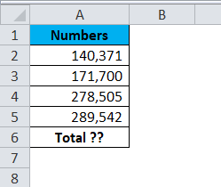
To get the total of the cells A2 to A5. I am going to apply the simple calculator method here. So the result will be:
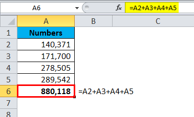
Firstly I selected the first number, cell A2; then I mentioned the addition symbol +, then I selected the second cell and again the + sign, and so on. This is as easy as you like.
The problem with this manual formula is that it will take a lot of time to apply in the case of many cells. I had only 4 cells to add in the above example, but what if there are 100 cells to add? It will be almost impossible to select one by one. That is why we have an inbuilt function called SUM function to deal with it.
The SUM function requires many parameters it the each is selected independently. If the range of cells is selected, it requires only one argument.
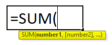
Number 1 is the first parameter. This is enough if the range of cells is selected, or else we need to keep mentioning the cells individually.
#Examples
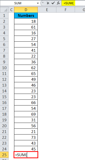
Look at the below example; it has data for 23 cells.
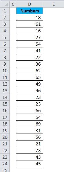
Now open the equal sign in cell D25 and type SUM.
Select the range of cells by holding the shift key.
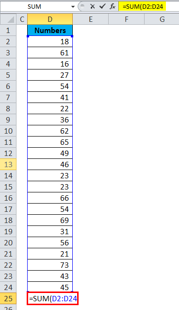
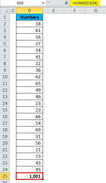
After selecting the range of cells to close the bracket and hit the enter button, it will give the summation for the numbers from D2 to D24.
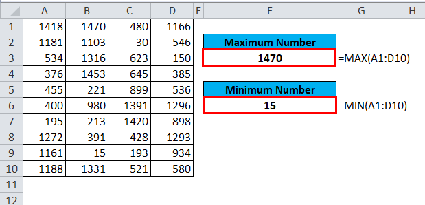
Formula #2 – MAX & MIN Function
If you are working with numbers, there are instances where you need to find the maximum number and the minimum number in the list. Look at the below data. I have few numbers from A1 to D10.
#Examples
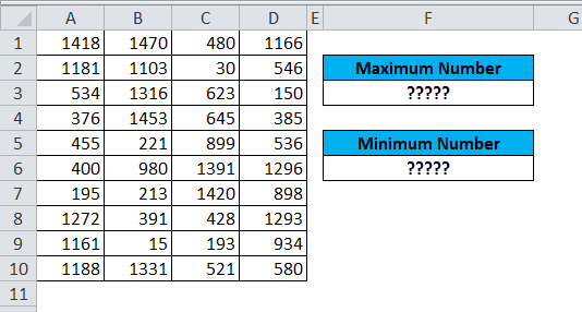
In cell F3, I want to know the maximum number in the list, and in cell F6, I want to know the minimum number. To find the maximum value, we have the MAX function; to find the minimum value, we have the MIN function.
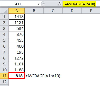
Formula #3 – AVERAGE Function
Finding the average of the list is easy in excel. Finding the average value can be done by using an AVERAGE function. Look at the below data. I have numbers from A1 to A10.
#Examples
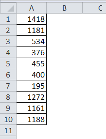
I am applying the AVERAGE function in the A11 cell. So the result will be:
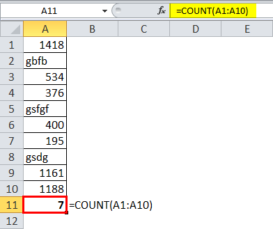
Formula #4 – COUNT Function
COUNT function will count the values in the supplied range. It will ignore text values in the range and count only numerical values.
Examples
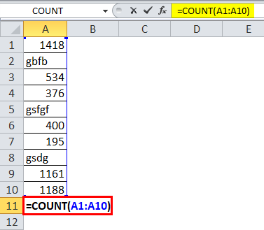
So the result will be:
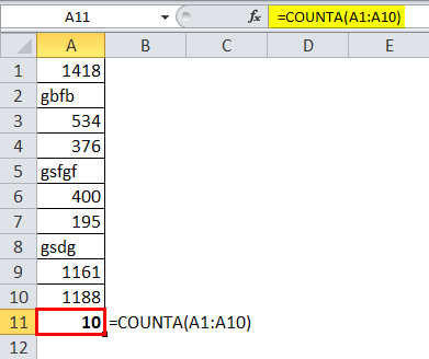
Formula #5 – COUNTA Function
COUNTA function counts all the things in the supplied range.
Examples
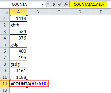
So the result will be:
Formula #6 – NOW Function
If you want to insert the current date and time, you can use the NOW function to do the task for you.
Examples
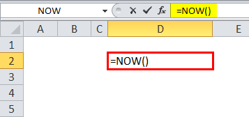
So the result will be:
Formula #7 – LEN Function
If you want to know how many characters are there in a cell, you can use the LEN function.
Examples
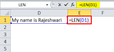
LEN function returns the length of the cell.
In the above image, I have applied the LEN function in cell E1 to find how many characters are there in cell D1. LEN function returns 21 as a result.
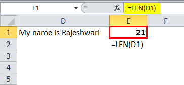
That means in cell D1 total of 21 characters are there, including space.
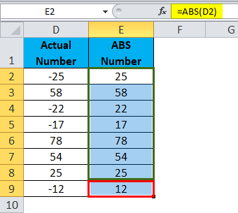
Formula #8 – ABS Function
You can use the ABS function to convert all the negative numbers to positive ones. ABS means absolute.
Examples
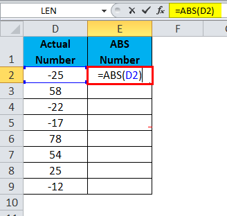
So the result will be:
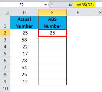
So the final output will occur by dragging cell E2.
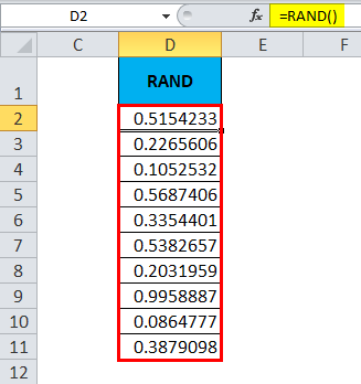
Formula #9 – RAND Function
RAND means random. You can use the RAND function to insert random numbers from 0 to less than 1. It is a volatile function.
Examples
Formula #10 – RANDBETWEEN Function
RAND function inserts the numbers from 0 to less than 1, but RANDBETWEEN inserts numbers based on the numbers we supply. We need to mention the bottom and top values to tell the function to insert random numbers between these two.
Examples
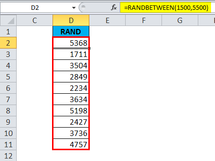
Look at the above image. I have mentioned the bottom value as 1500 and the top value as 5500. Formula inserted numbers between these two numbers.
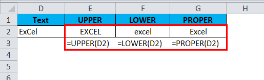
Formula #11 – UPPER, LOWER & PROPER Function
When you are dealing with the text values, we care about their appearances. If we want to convert the text to UPPERCASE, we can use an UPPER function, we want to convert the text to LOWERCASE, we can use the LOWER function, and if we want to make the text proper appearance, we can use the PROPER function.
Examples
Errors in excel formulas
How many times have you encountered Excel errors? It’s a frustrating experience when Excel gives an error. Mostly two kinds of Excel formulas error occurs in Excel first is #VALUE And #NAME. This will happen if the formula you’ve typed is invalid.
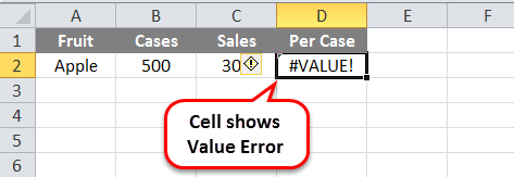
#VALUE Error
This means that you have entered a formula that was valued, but Excel could not calculate a valid result from your formula.
Look at the following picture carefully; there are two columns consist of the Department and the number of students. Now #VALUE error occurs when you try to calculate Excel formulas to add cells containing the non-numerical value. If you are trying to Add values Cell A2 and B2, then Excel gives you the #VALUE error because Cell A2 contains the non-numerical value.
Reasons for #VALUE Error
- Adding cells that contain a non-numerical value.
- Error with formula
- Non-numerical value
This Excel formula error is commonly encountered when the formula isn’t formatted correctly or contains other errors, as seen in the example below.
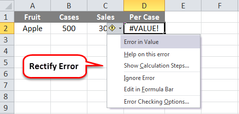
How to Correct #VALUE Error
Instead of using arithmetic operators, use a function, such as SUM, PRODUCT, or QUOTIENT, to perform an arithmetic operation. Ensure that adding cell does not contain a non-numerical value. The following picture shows how to correct the #VALUE error. In the above example, we have seen why a #VALUE error occurs. Now We are trying to Add cells, including numerical values only. In short, we can say that avoid addition, subtraction, division, or multiplication of non-numerical values with numerical values.
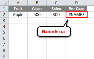
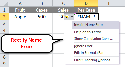
#NAME Error
#NAME error occurs when Excel doesn’t recognize text in a formula. Look at the following picture. If we want to calculate Excel formulas for the sum of a number of students, then what do we do? We insert the SUM formula, then select range and press enter. But if you enter formula SUM and select range, then press enter. Excel gives an #NAME error. Because you enter the wrong formula.
How to Correct #NAME Error
- Ensure the formula is correctly entered.
- Make sure quotation marks are added and balanced from left and right.
- Replacing a colon (:) in a range reference. For e.g. SUM(A1A10) should be COUNT(A1: A10)
Some Basic Arithmetic Excel Formulas
Arithmetic formulas are by far the most common type of formula. It generally includes mathematical operators like Addition, Subtraction, Multiplication, Division, etc., to perform calculations. Look at the following table.
The Arithmetic Operators
| Operator | Name | Example | Result |
|---|---|---|---|
| + | Addition | =5+5 | 10 |
| – | Subtraction | =10-5 | 5 |
| – | Negation | =-10 | -10 |
| * | Multiplication | =10*5 | 50 |
| / | Division | =10/5 | 2 |
| % | Percentage | =10% | 0.1 |
| ^ | Exponentiation | =10^5 | 100000 |
Top 10 Basic Excel Formulas That You Should Know
Don’t waste any more hours in Microsoft Excel doing things manually. Excel formulas decrease the amount of time you spend in Excel and increase the accuracy of your data and your reports.
| Name of Formulas | Formula | Description |
|---|---|---|
| SUM | =SUM ( Number1, Number2, … ) | Add all numbers within range resulted into the sum of all numbers |
| AVERAGE | =AVERAGE(number1, [number2],…) | Calculate average numbers in a range |
| MAX | =MAX( Number1, Number2, … ) | Calculate or find the largest number in a specific range |
| MIN | =MIN( Number1, Number2, … ) | Calculate or find the smallest number in a specific range |
| TODAY | =TODAY() | Returns the current date |
| UPPER | =UPPER(text) | Converts text to uppercase. |
| LOWER | =LOWER(text) | Converts text into lowercase. |
| Countif | =COUNTIF(range, criteria) | This function counts the number of cells within a range that meet a single criterion that you specify. |
| counta | = COUNTA(value1, [value2], …) | This function counts the number of cells that are not empty in a range. |
| ABS | = ABS(number) | ABS function returns a value of the same type that is passed to it, specifying the absolute value of a number. |
Recommended Free Formulas Training:
If you simply search on Google for free Excel courses, you may get a long list of free Excel training courses. However, you might get confused by referring to so many Excel resources. I suggest you go for EduCBA’s free online training on Excel. Online courses are much better than some of the expensive classroom training courses because they provide time flexibility and cost-effectiveness. The Excel formulas learning materials are freely available on the EduCBA website, and the videos include in the course are short and very easy to understand, planned especially for beginners. Also, for your convenience, the spreadsheets explained in the videos are available for download. This way, you can immediately practice what you have just seen and learned.
Free Demo Excel:-
Recommended Articles
Here are some articles that will help you to get more detail about the Excel Formulas Useful For Any Professionals, so go through the link.
- Benefits of Microsoft Excel Tips and Tricks (Spreadsheet)
- Popular Things About Excel VBA Macro
- Excel Use formulas with Conditional Formatting (Examples)
- Top 25 Useful Advanced Excel Formulas and Functions
- 8 Awesome & Useful Features of 2016 Excel Workbook