
In PivotTables, you can use summary functions in value fields to combine values from the underlying source data. If summary functions and custom calculations do not provide the results that you want, you can create your own formulas in calculated fields and calculated items. For example, you could add a calculated item with the formula for the sales commission, which could be different for each region. The PivotTable would then automatically include the commission in the subtotals and grand totals.
Another way to calculate is to use Measures in Power Pivot, which you create using a Data Analysis Expressions (DAX) formula. For more information, see Create a Measure in Power Pivot.
PivotTables provide ways to calculate data. Learn about the calculation methods that are available, how calculations are affected by the type of source data, and how to use formulas in PivotTables and PivotCharts.
To calculate values in a PivotTable, you can use any or all of the following types of calculation methods:
-
Summary functions in value fields The data in the values area summarize the underlying source data in the PivotTable. For example, the following source data:

-
Produces the following PivotTables and PivotCharts. If you create a PivotChart from the data in a PivotTable, the values in that PivotChart reflect the calculations in the associated PivotTable report.
-
In the PivotTable, the Month column field provides the items March and April. The Region row field provides the items North, South, East, and West. The value at the intersection of the April column and the North row is the total sales revenue from the records in the source data that have Month values of April and Region values of North.
-
In a PivotChart, the Region field might be a category field that shows North, South, East, and West as categories. The Month field could be a series field that shows the items March, April, and May as series represented in the legend. A Values field named Sum of Sales could contain data markers that represent the total revenue in each region for each month. For example, one data marker would represent, by its position on the vertical (value) axis, the total sales for April in the North region.
-
To calculate the value fields, the following summary functions are available for all types of source data except Online Analytical Processing (OLAP) source data.
Function
Summarizes
Sum
The sum of the values. This is the default function for numeric data.
Count
The number of data values. The Count summary function works the same as the COUNTA function. Count is the default function for data other than numbers.
Average
The average of the values.
Max
The largest value.
Min
The smallest value.
Product
The product of the values.
Count Nums
The number of data values that are numbers. The Count Nums summary function works the same as the COUNT function.
StDev
An estimate of the standard deviation of a population, where the sample is a subset of the entire population.
StDevp
The standard deviation of a population, where the population is all of the data to be summarized.
Var
An estimate of the variance of a population, where the sample is a subset of the entire population.
Varp
The variance of a population, where the population is all of the data to be summarized.
-
Custom calculations A custom calculation shows values based on other items or cells in the data area. For example, you could display values in the Sum of Sales data field as a percentage of March sales, or as a running total of the items in the Month field.
The following functions are available for custom calculations in value fields.
Function
Result
No Calculation
Displays the value that is entered in the field.
% of Grand Total
Displays values as a percentage of the grand total of all of the values or data points in the report.
% of Column Total
Displays all of the values in each column or series as a percentage of the total for the column or series.
% of Row Total
Displays the value in each row or category as a percentage of the total for the row or category.
% Of
Displays values as a percentage of the value of the Base item in the Base field.
% of Parent Row Total
Calculates values as follows:
(value for the item) / (value for the parent item on rows)
% of Parent Column Total
Calculates values as follows:
(value for the item) / (value for the parent item on columns)
% of Parent Total
Calculates values as follows:
(value for the item) / (value for the parent item of the selected Base field)
Difference From
Displays values as the difference from the value of the Base item in the Base field.
% Difference From
Displays values as the percentage difference from the value of the Base item in the Base field.
Running Total in
Displays the value for successive items in the Base field as a running total.
% Running Total in
Calculates the value for successive items in the Base field that are displayed as a running total as a percentage.
Rank Smallest to Largest
Displays the rank of selected values in a specific field, listing the smallest item in the field as 1, and each larger value will have a higher rank value.
Rank Largest to Smallest
Displays the rank of selected values in a specific field, listing the largest item in the field as 1, and each smaller value will have a higher rank value.
Index
Calculates values as follows:
((value in cell) x (Grand Total of Grand Totals)) / ((Grand Row Total) x (Grand Column Total))
-
Formulas If summary functions and custom calculations do not provide the results that you want, you can create your own formulas in calculated fields and calculated items. For example, you could add a calculated item with the formula for the sales commission, which could be different for each region. The report would then automatically include the commission in the subtotals and grand totals.
Calculations and options that are available in a report depend on whether the source data came from an OLAP database or a non-OLAP data source.
-
Calculations based on OLAP source data For PivotTables that are created from OLAP cubes, the summarized values are precalculated on the OLAP server before Excel displays the results. You cannot change how these precalculated values are calculated in the PivotTable. For example, you cannot change the summary function that is used to calculate data fields or subtotals, or add calculated fields or calculated items.
Also, if the OLAP server provides calculated fields, known as calculated members, you will see these fields in the PivotTable Field List. You will also see any calculated fields and calculated items that are created by macros that were written in Visual Basic for Applications (VBA) and stored in your workbook, but you won’t be able to change these fields or items. If you need additional types of calculations, contact your OLAP database administrator.
For OLAP source data, you can include or exclude the values for hidden items when calculating subtotals and grand totals.
-
Calculations based on non-OLAP source data In PivotTables that are based on other types of external data or on worksheet data, Excel uses the Sum summary function to calculate value fields that contain numeric data, and the Count summary function to calculate data fields that contain text. You can choose a different summary function, such as, Average, Max, or Min, to further analyze and customize your data. You can also create your own formulas that use elements of the report or other worksheet data by creating a calculated field or a calculated item within a field.
You can create formulas only in reports that are based on a non-OLAP source data. You cannot use formulas in reports that are based on an OLAP database. When you use formulas in PivotTables, you should know about the following formula syntax rules and formula behavior:
-
PivotTable formula elements In formulas that you create for calculated fields and calculated items, you can use operators and expressions as you do in other worksheet formulas. You can use constants and refer to data from the report, but you cannot use cell references or defined names. You cannot use worksheet functions that require cell references or defined names as arguments, and you cannot use array functions.
-
Field and item names Excel uses field and item names to identify those elements of a report in your formulas. In the following example, the data in range C3:C9 is using the field name Dairy. A calculated item in the Type field that estimates sales for a new product based on Dairy sales could use a formula such as =Dairy * 115%.
Note: In a PivotChart, the field names are displayed in the PivotTable field list, and item names can be seen in each field drop-down list. Don’t confuse these names with those you see in chart tips, which reflect series and data point names instead.
-
Formulas operate on sum totals, not individual records Formulas for calculated fields operate on the sum of the underlying data for any fields in the formula. For example, the calculated field formula =Sales * 1.2 multiplies the sum of the sales for each type and region by 1.2; it does not multiply each individual sale by 1.2 and then sum the multiplied amounts.
Formulas for calculated items operate on the individual records. For example, the calculated item formula =Dairy *115% multiplies each individual sale of Dairy times 115%, after which the multiplied amounts are summarized together in the Values area.
-
Spaces, numbers, and symbols in names In a name that includes more than one field, the fields can be in any order. In the example above, cells C6:D6 can be ‘April North’ or ‘North April’. Use single quotation marks around names that are more than one word or that include numbers or symbols.
-
Totals Formulas cannot refer to totals (such as, March Total, April Total, and Grand Total in the example).
-
Field names in item references You can include the field name in a reference to an item. The item name must be in square brackets — for example, Region[North]. Use this format to avoid #NAME? errors when two items in two different fields in a report have the same name. For example, if a report has an item named Meat in the Type field and another item named Meat in the Category field, you can prevent #NAME? errors by referring to the items as Type[Meat] and Category[Meat].
-
Referring to items by position You can refer to an item by its position in the report as currently sorted and displayed. Type[1] is Dairy, and Type[2] is Seafood. The item referred to in this way can change whenever the positions of items change or different items are displayed or hidden. Hidden items are not counted in this index.
You can use relative positions to refer to items. The positions are determined relative to the calculated item that contains the formula. If South is the current region, Region[-1] is North; if North is the current region, Region[+1] is South. For example, a calculated item could use the formula =Region[-1] * 3%. If the position that you give is before the first item or after the last item in the field, the formula results in a #REF! error.
To use formulas in a PivotChart, you create the formulas in the associated PivotTable, where you can see the individual values that make up your data, and then you can view the results graphically in the PivotChart.
For example, the following PivotChart shows sales for each salesperson per region:
To see what sales would look like if they were increased by 10 percent, you could create a calculated field in the associated PivotTable that uses a formula such as =Sales * 110%.
The result immediately appears in the PivotChart, as shown in the following chart:
To see a separate data marker for sales in the North region minus a transportation cost of 8 percent, you could create a calculated item in the Region field with a formula such as =North – (North * 8%).
The resulting chart would look like this:
However, a calculated item that is created in the Salesperson field would appear as a series represented in the legend and appear in the chart as a data point in each category.
Important: You cannot create formulas in a PivotTable that is connected to an Online Analytical Processing (OLAP) data source.
Before you start, decide whether you want a calculated field or a calculated item within a field. Use a calculated field when you want to use the data from another field in your formula. Use a calculated item when you want your formula to use data from one or more specific items within a field.
For calculated items, you can enter different formulas cell by cell. For example, if a calculated item named OrangeCounty has a formula of =Oranges * .25 across all months, you can change the formula to =Oranges *.5 for June, July, and August.
If you have multiple calculated items or formulas, you can adjust the order of calculation.
Add a calculated field
-
Click the PivotTable.
This displays the PivotTable Tools, adding the Analyze and Design tabs.
-
On the Analyze tab, in the Calculations group, click Fields, Items, & Sets, and then click Calculated Field.
-
In the Name box, type a name for the field.
-
In the Formula box, enter the formula for the field.
To use the data from another field in the formula, click the field in the Fields box, and then click Insert Field. For example, to calculate a 15% commission on each value in the Sales field, you could enter = Sales * 15%.
-
Click Add.
Add a calculated item to a field
-
Click the PivotTable.
This displays the PivotTable Tools, adding the Analyze and Design tabs.
-
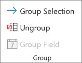
If items in the field are grouped, on the Analyze tab, in the Group group, click Ungroup.
-
Click the field where you want to add the calculated item.
-
On the Analyze tab, in the Calculations group, click Fields, Items, & Sets, and then click Calculated Item.
-
In the Name box, type a name for the calculated item.
-
In the Formula box, enter the formula for the item.
To use the data from an item in the formula, click the item in the Items list, and then click Insert Item (the item must be from the same field as the calculated item).
-
Click Add.
Enter different formulas cell by cell for calculated items
-
Click a cell for which you want to change the formula.
To change the formula for several cells, hold down CTRL and click the additional cells.
-
In the formula bar, type the changes to the formula.
Adjust the order of calculation for multiple calculated items or formulas
-
Click the PivotTable.
This displays the PivotTable Tools, adding the Analyze and Design tabs.
-
On the Analyze tab, in the Calculations group, click Fields, Items, & Sets, and then click Solve Order.
-
Click a formula, and then click Move Up or Move Down.
-
Continue until the formulas are in the order that you want them to be calculated.
You can display a list of all the formulas that are used in the current PivotTable.
-
Click the PivotTable.
This displays the PivotTable Tools, adding the Analyze and Design tabs.
-
On theAnalyze tab, in the Calculations group, click Fields, Items, & Sets, and then click List Formulas.
Before you edit a formula, determine whether that formula is in a calculated field or a calculated item. If the formula is in a calculated item, also determine whether the formula is the only one for the calculated item.
For calculated items, you can edit individual formulas for specific cells of a calculated item. For example, if a calculated item named OrangeCalc has a formula of =Oranges * .25 across all months, you can change the formula to =Oranges *.5 for June, July, and August.
Determine whether a formula is in a calculated field or a calculated item
-
Click the PivotTable.
This displays the PivotTable Tools, adding the Analyze and Design tabs.
-
On the Analyze tab, in the Calculations group, click Fields, Items, & Sets, and then click List Formulas.
-
In the list of formulas, find the formula that you want to change listed under Calculated Field or Calculated Item.
When there are multiple formulas for a calculated item, the default formula that was entered when the item was created has the calculated item name in column B. For additional formulas for a calculated item, column B contains both the calculated item name and the names of intersecting items.
For example, you might have a default formula for a calculated item named MyItem, and another formula for this item identified as MyItem January Sales. In the PivotTable, you would find this formula in the Sales cell for the MyItem row and January column.
-
Continue by using one of the following editing methods.
Edit a calculated field formula
-
Click the PivotTable.
This displays the PivotTable Tools, adding the Analyze and Design tabs.
-
On the Analyze tab, in the Calculations group, click Fields, Items, & Sets, and then click Calculated Field.
-
In the Name box, select the calculated field for which you want to change the formula.
-
In the Formula box, edit the formula.
-
Click Modify.
Edit a single formula for a calculated item
-
Click the field that contains the calculated item.
-
On the Analyze tab, in the Calculations group, click Fields, Items, & Sets, and then click Calculated Item.
-
In the Name box, select the calculated item.
-
In the Formula box, edit the formula.
-
Click Modify.
Edit an individual formula for a specific cell of a calculated item
-
Click a cell for which you want to change the formula.
To change the formula for several cells, hold down CTRL and click the additional cells.
-
In the formula bar, type the changes to the formula.
Tip: If you have multiple calculated items or formulas, you can adjust the order of calculation. For more information, see Adjust the order of calculation for multiple calculated items or formulas.
Note: Deleting a PivotTable formula removes it permanently. If you do not want to remove a formula permanently, you can hide the field or item instead by dragging it out of the PivotTable.
-
Determine whether the formula is in a calculated field or a calculated item.
Calculated fields appear in the PivotTable Field List. Calculated items appear as items within other fields.
-
Do one of the following:
-
To delete a calculated field, click anywhere in the PivotTable.
-
To delete a calculated item, in the PivotTable, click the field that contains the item that you want to delete.
This displays the PivotTable Tools, adding the Analyze and Design tabs.
-
-
On the Analyze tab, in the Calculations group, click Fields, Items, & Sets, and then click Calculated Field or Calculated Item.
-
In the Name box, select the field or item that you want to delete.
-
Click Delete.
To summarize values in a PivotTable in Excel for the web, you can use summary functions like Sum, Count, and Average. The Sum function is used by default for numeric values in value fields. You can view and edit a PivotTable based on an OLAP data source, but you can’t create one in Excel for the web.
Here’s how to choose a different summary function:
-
Click anywhere on the PivotTable, and then select PivotTable > Field List. You can also right-click the PivotTable and then select Show Field List.
-
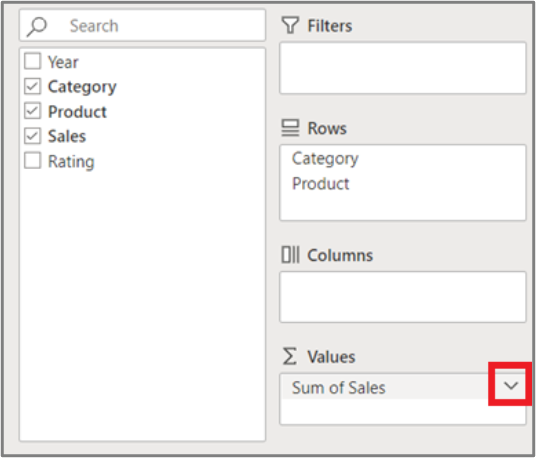
In the PivotTable Fields list, under Values, click the arrow next to the value field.
-
Click Value Field Settings.
-
Pick the summary function you want and then click OK.
Note: Summary functions aren’t available in PivotTables that are based on Online Analytical Processing (OLAP) source data.
Use this summary function
To calculate
Sum
The sum of the values. It’s used by default for value fields that have numeric values.
Count
The number of nonempty values. The Count summary function works the same as the COUNTA function. Count is used by default for value fields that have nonnumeric values or blanks.
Average
The average of the values.
Max
The largest value.
Min
The smallest value.
Product
The product of the values.
Count Numbers
The number of values that contain numbers (not the same as Count, which includes nonempty values).
StDev
An estimate of the standard deviation of a population, where the sample is a subset of the entire population.
StDevp
The standard deviation of a population, where the population is all of the data to be summarized.
Var
An estimate of the variance of a population, where the sample is a subset of the entire population.
Varp
The variance of a population, where the population is all of the data to be summarized.
Need more help?
You can always ask an expert in the Excel Tech Community or get support in the Answers community.
Often, once you create a Pivot table, there is a need you to expand your analysis and include more data/calculations as a part of it.
If you need a new data point that can be obtained by using existing data points in the Pivot Table, you don’t need to go back and add it in the source data. Instead, you can use a Pivot Table Calculated Field to do this.
Download the dataset and follow along.
What is a Pivot Table Calculated Field?
Let’s start with a basic example of a Pivot Table.
Suppose you have a dataset of retailers and you create a Pivot Table as shown below:
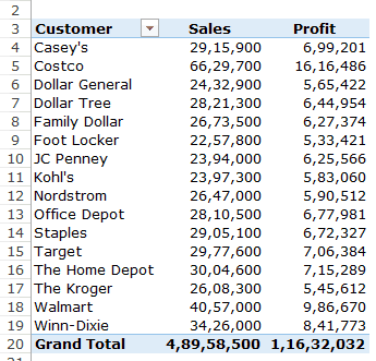
The above Pivot Table summarizes the sales and profit values for the retailers.
Now, what if you also want to know what was the profit margin of these retailers (where the profit margin is ‘Profit’ divided by ‘Sales’).
There are a couple of ways to do this:
- Go back to the original data set and add this new data point. So you can insert a new column in the source data and calculate the profit margin in it. Once you do this, you need to update the source data of the Pivot Table to get this new column as a part of it.
- While this method is a possibility, you would need to manually go back to the data set and make the calculations. For example, you may need to add another column to calculate the average sale per unit (Sales/Quantity). Again you will have to add this column to your source data and then update the pivot table.
- This method also bloats your Pivot Table as you’re adding new data to it.
- Add calculations outside the Pivot Table. This can be an option if your Pivot Table structure is unlikely to change. But if you change the Pivot table, the calculation may not update accordingly and might give you the wrong results or errors. As shown below, I calculated the Profit Margin when there were retailers in the row. But when I changed it from customers to regions, the formula gave an error.

- Using a Pivot Table Calculated Field. This is the most efficient way to use existing Pivot Table data and calculate the desired metric. Consider Calculated Field as a virtual column that you have added using the existing columns from the Pivot Table. There are a lot of benefits of using a Pivot Table Calculated Field (as we will see in a minute):
- It doesn’t require you to handle formulas or update source data.
- It’s scalable as it will automatically account for any new data that you may add to your Pivot Table. Once you add a Calculate Field, you can use it like any other field in your Pivot Table.
- It easy to update and manage. For example, if the metrics change or you need to change the calculation, you can easily do that from the Pivot Table itself.

Adding a Calculated Field to the Pivot Table
Let’s see how to add a Pivot Table Calculated Field in an existing Pivot Table.
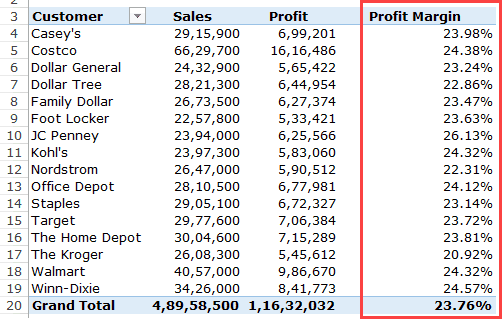
Suppose you have a Pivot Table as shown below and you want to calculate the profit margin for each retailer:
Here are the steps to add a Pivot Table Calculated Field:
As soon as you add the Calculated Field, it will appear as one of the fields in PivotTable Fields list.

Now you can use this calculated field as any other Pivot Table field (note that you can not use Pivot Table Calculated Field as a report filter or slicer).
As I mentioned before, the benefit of using a Pivot Table Calculated Field is that you can change the structure of the Pivot Table and it will automatically adjust.
For example, if I drag and drop region in the rows area, you will get the result as shown below, where Profit Margin value is reported for retailers as well as the region.
 In the above example, I have used a simple formula (=Profit/Sales) to insert a calculated field. However, you can also use some advanced formulas.
Before I show you an example of using an advanced formula to create a Pivot Table Calculate Field, here are some things you must know:
- You CAN NOT use references or named ranges while creating a Pivot Table Calculated Field. That would rule out a lot of formulas such as VLOOKUP, INDEX, OFFSET, and so on. However, you can use formulas that can work without references (such SUM, IF, COUNT, and so on..).
- You can use a constant in the formula. For example, if you want to know the forecasted sales where it is forecasted to grow by 10%, you can use the formula =Sales*1.1 (where 1.1 is constant).
- The order of precedence is followed in the formula that makes the calculated field. As a best practice, use parenthesis to make sure you don’t have to remember the order of precedence.
Now, let’s see an example of using an advanced formula to create a Calculated Field.
Suppose you have the dataset as shown below and you need to show the forecasted sales value in the Pivot Table.
For forecasted value, you need to use a 5% sales increase for large retailers (sales above 3 million) and a 10% sales increase for small and medium retailers (sales below 3 million).
Note: The sales numbers here are fake and have been used to illustrate the examples in this tutorial.
Here is how to do this:
This adds a new column to the pivot table with the sales forecast value.
Click here to Download the dataset.
An Issue With Pivot Table Calculated Fields
Calculated Field is an amazing feature that really enhances the value of your Pivot Table with field calculations, while still keep everything scalable and manageable.
There is, however, an issue with Pivot Table Calculated Fields that you must know before using it.
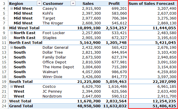
Suppose, I have a Pivot Table as shown below where I used the calculated field to get the forecast sales numbers.
Note that the subtotal and grand totals are not correct.
While these should add the individual sales forecast value for each retailer, in reality, it follows the same calculated field formula that we created.
So for South Total, while the value should be 22,824,000, the South Total wrongly reports it as 22,287,000. This happens as it uses the formula 21,225,800*1.05 to get the value.

Unfortunately, there is no way you can correct this.
The best way to handle this would be to remove subtotals and Grand Totals from your Pivot Table.
You can also go through some innovative workarounds Debra has shown to handle this issue.
How to Modify or Delete a Pivot Table Calculated Field?
Once you have created a Pivot Table Calculated Field, you can modify the formula or delete it using the following steps:
How to Get a List of All the Calculated Field Formulas?
If you create a lot of Pivot Table Calculated field, don’t worry about keeping track of the formula used in each one of it.
Excel allows you to quickly create a list of all the formulas used in creating Calculated Fields.
Here are the steps to quickly get the list of All Calculated Fields formulas:
- Select any cell in the Pivot Table.
- Go to Pivot Table Tools –> Analyze –> Fields, Items, & Sets –> List Formulas.

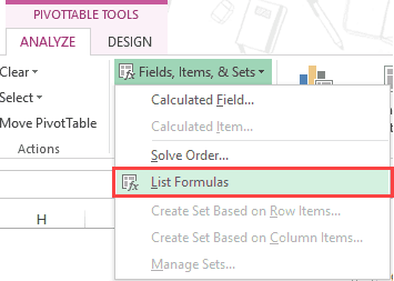
As soon as you click on List Formulas, Excel would automatically insert a new worksheet that will have the details of all the calculated fields/items that you have used in the Pivot Table.
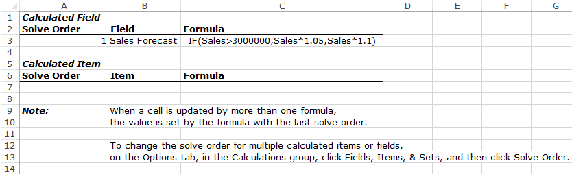
This can be a really useful tool if you have to send your work to the client or share it with your team.
You May Also Find the following Pivot Table Tutorials Useful:
- Preparing Source Data For Pivot Table.
- Using Slicers in Excel Pivot Table: A Beginner’s Guide.
- How to Group Dates in Pivot Tables in Excel.
- How to Group Numbers in Pivot Table in Excel.
- How to Filter Data in a Pivot Table in Excel.
- How to Replace Blank Cells with Zeros in Excel Pivot Tables.
- How to Apply Conditional Formatting in a Pivot Table in Excel.
- Pivot Cache in Excel – What Is It and How to Best Use It?
- How to Delete a Pivot Table in Excel
- How to Show Pivot Table Fields List? (Get Pivot Table Menu Back)
Home / Pivot Table / Formulas in a Pivot Table (Calculated Fields & Items)
One of the best ways to become an advanced pivot table user and use Excel for data analysis is by using calculated items and calculated fields in a pivot table.
Using formulas in a pivot table or custom calculation which don’t exist in the source data but work like other fields.
In simple words, these are the calculations within the pivot table. In the below example, you can see a pivot table with a calculated field which is calculating the average selling price. On the other hand, source data doesn’t have any type of field like this.

Pivot Tables are one of the INTERMEDIATE EXCEL SKILLS.
In the Excel pivot table, the calculated field is like all other fields of your pivot table, but they don’t exist in the source data. But, they are created by using formulas in the pivot table. Follow these simple steps to insert the calculated field in a pivot table.
- First of all, you need a simple pivot table to add a Calculated Field.
- Just click on any of the fields in your pivot table. You will see a pivot table option in your ribbon which further having further two options (Analyze & Design) Click on the analyze option, then on Fields, Items, & Sets. You will further get a list of options, just click on the calculated field.
- After clicking the calculated field, you will get a pop-up menu, just like below. This popup menu comes with two input options (name & formula) & a selection option.
- Name: Name of the calculated Field which will show in your pivot table.
- Formula: An input option to insert formula for calculated field.
- Fields: A drop down option to select other fields from source data to calculate a new field.


Calculated Items in a Pivot Table
Calculated items are like all other items of your pivot table, but the difference is that they are not in existence in your source data. They are just created by using a formula. You can edit, change or delete calculated Items as per your requirement.
- Just click on any of the items in your pivot table. You will see a pivot table option on your ribbon having further two options (Analyze & Design).
- Click on the Analyze, then on Fields, Items, & Sets.
- You will further get a list of options, just click on Calculated Item.
- After clicking the calculated item, you will get a pop-up menu, just like above. This popup menu comes with two input options (Name & Formula) & two selection options (Field & Items).
- We had already discussed “Name, Formula & Fields” in calculated fields.
- Items: To select the items for calculation.
- In this example, we are going to calculate the average selling price and, the formula will be = amount/quantity.
- In Fields option, select Amount & click on insert, then insert “/” division operator & insert quantity after that.
- Press OK.
- Now a new Field appears in your Pivot Table.
- Your new calculated field is created without any number format.


In this example, we are going to calculate the average for the first half of the year & for the 2nd half of the year. We just have to add the formula.
=average(jan, feb, mar, apr, may, jun)Now you have to calculate items in your pivot, showing an average of the first six months and the second six months of the year.

But wait a minute. What is this? Grand total is changed from 1506 & $311820 to 1746 & $361600.

The reason behind this is, pivot table totals & subtotals include your calculated fields while the calculation of total and sub-total. So you need to filter your calculated items if you want to show the actual picture.
Things To Remember
- Don’t forget to remove 0 from the formula input option while inserting a formula for calculation
- You can only able to use formulas that don’t require cell references.
- You have to check whether calculated items are affecting your pivot results (Sub Totals and Grand Totals).
- Adjust the solve order are per your calculation requirement.
How To Add A Calculated Field In Pivot Table?
Below are the examples of the PivotTable calculated field and how to insert formulas on other Pivot fields.
Table of contents
- How To Add A Calculated Field In Pivot Table?
- Using Manual Reference of Cell in the Pivot Table Formula
- Using GetPivotTable Function to give Reference of a Cell to a Formula
- Switching off the “GetPivot” table Function in a Pivot Table to have a Clean Formula
- Things to Remember
- Recommended Articles
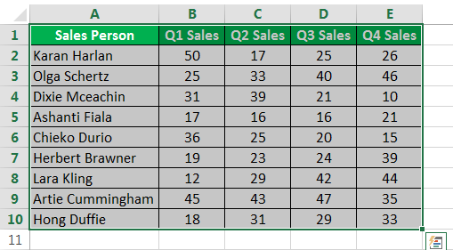
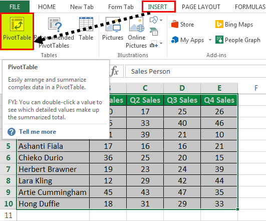
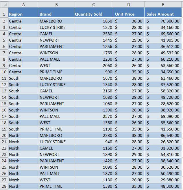
- Select the data that is to be used in a PivotTable.

- Go to the ribbon and select the “Insert” tab. From the “Insert” tab, choose to insert a “PivotTable.”

- Select the “PivotTable Fields” such as “Sales Person” to the “ROWS” and Q1, Q2, Q3, and Q4 sales to the “Values.”

Now, the PivotTable is ready.

- After the PivotTable is inserted, go to the “Analyze” tab that will only be present if the PivotTable is selected.

- From the “PivotTable Analyze” tab, choose the option of “Fields, Items Sets” and select the “Calculated Field” of the PivotTable.

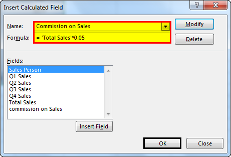
- In the option of “Insert Calculated Field” in the Pivot Table, insert the formula as required in the case.

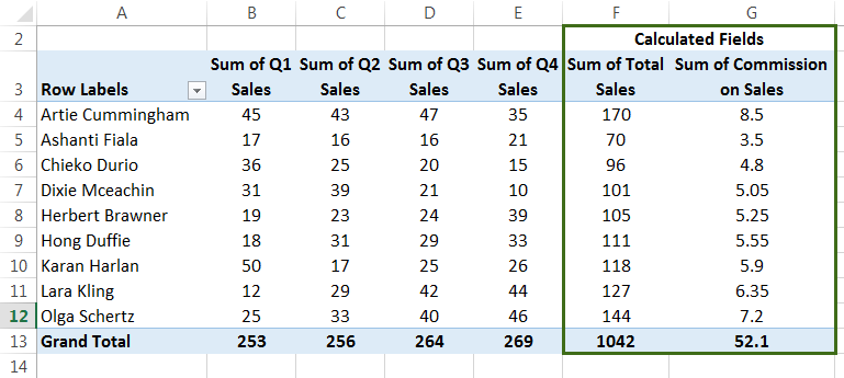
Here, we have formulated a formula to calculate the 0.05% commission on sales.


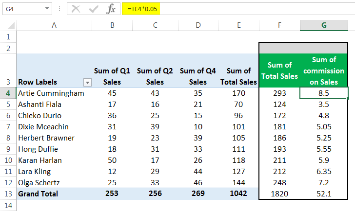
Using Manual Reference of Cell in the Pivot Table Formula
If we have to give a cell reference in a formula, we can type the location as shown below.
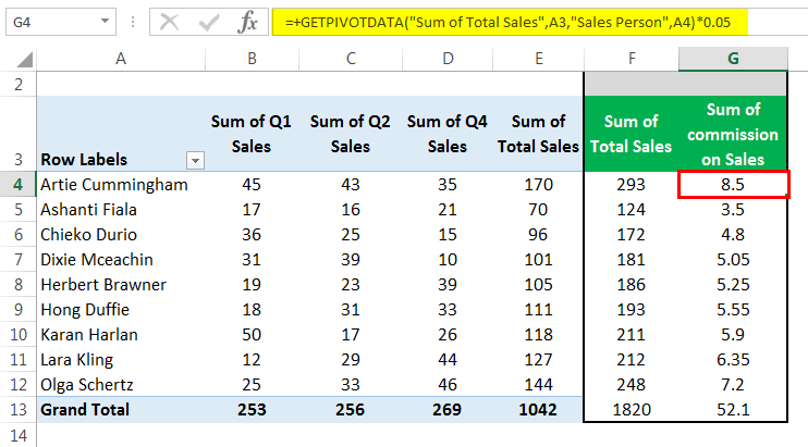
Using GetPivotTable Function to give Reference of a Cell to a Formula
We can also choose not to enter the cell’s location manually. In this case, we can choose to insert the location by using the keyboard instead of a mouse.
This type of location (GetpivotDataThe GetPivotData function in Excel is a query function that fetches values from a pivot table based on specific criteria such as the pivot table’s structure or the reference provided to the function.read more) is inserted if we select the location instead of manually typing the cell’s location.
Switching off the “GetPivot” table Function in a Pivot Table to have a Clean Formula
We can always switch off the “Getpivotdata” function by selecting the “Analyze” tab and selecting the dropdown.

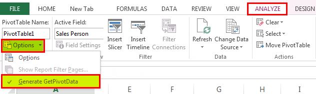
Here, we need to turn off the “Generate GetPivotData” option, and we can use the formulas in the PivotTable as we do in the case of a simple range.
You can download this Pivot Table Calculated Field Excel template here – Pivot Table Calculated Field Excel template
Things to Remember
- We can use some basic mathematical operations inside the calculated fields in the Pivot TableA Pivot Table is an Excel tool that allows you to extract data in a preferred format (dashboard/reports) from large data sets contained within a worksheet. It can summarize, sort, group, and reorganize data, as well as execute other complex calculations on it.read more. However, we cannot use the logical and other thread functions.
- A Cell referenceCell reference in excel is referring the other cells to a cell to use its values or properties. For instance, if we have data in cell A2 and want to use that in cell A1, use =A2 in cell A1, and this will copy the A2 value in A1.read more will not change if the reference is generated via the GETPIVOTDATA function.
- The calculated field formulas are also a part of a PivotTable.
- If there is a change in the source data, then the formulas will be unchanged until the pivot table is refreshedTo refresh pivot tables, you may use the following methods — refresh pivot table by changing data source, refresh pivot table using right click option, auto-refresh pivot table using VBA Code, refresh pivot table when you open the workbook.read more.
Recommended Articles
This article is a guide to PivotTable Calculated Field. Here we discuss formulas in the PivotTable using calculated fields, practical examples, and a downloadable Excel template. You may learn more about Excel from the following articles: –
- Pivot Table From Multiple SheetsPivot Table is a basic data analysis tool that calculates, summarizes, & analyses the data of a more extensive table. To create a Pivot Table from Multiple Sheets, you can use a few shortcuts & features as per the specified conditions. read more
- Filter in Pivot TableBy right-clicking on the pivot table, we can access the pivot table filter option. Another approach is to use the filter options available in the pivot table fields.read more
- Pivot Chart in ExcelIn Excel, a pivot chart is a built-in feature that allows you to summarize selected rows and columns of data in a spreadsheet. It is a visual representation of a pivot table that helps in the summarization and analysis of datasets, patterns, and trends.read more
- Moving Average in ExcelMoving average means we calculate the average of the averages of the data set we have, in excel we have an inbuilt feature for the calculation of moving average which is available in the data analysis tab in the analysis section, it takes an input range and output range with intervals as an output, calculations based on mere formulas in excel to calculate moving average is hard but we have an inbuilt function in excel to do so.read more
Reader Interactions
In Excel, Pivot table Calculated Fields can be added as new fields in a Pivot table. These contain values based on calculations performed on data from Pivot table field(s). Calculated Fields do not contain any data themselves, but these fields derive data based on formula calculations on Pivot table field(s).
Calculated fields in Excel Pivot Tables
Calculated Fields use all the data of certain Pivot Table’s Field(s) and execute the calculation based on the supplied formula. Calculated Fields can add/ subtract/multiply/divide the values of already present data fields. In this article, you will learn how to create, modify and delete a Calculated Field in a Pivot table.
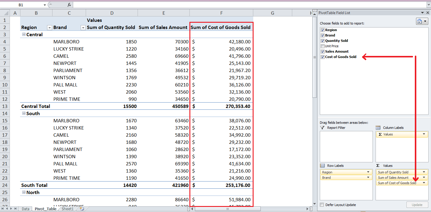
Let’s assume you are working in a company who sells different brands of cigarettes in different regions. You have a dataset of Sales that contains data fields of Region, Brand, Quantity Sold, Unit Price and Sales Amount.
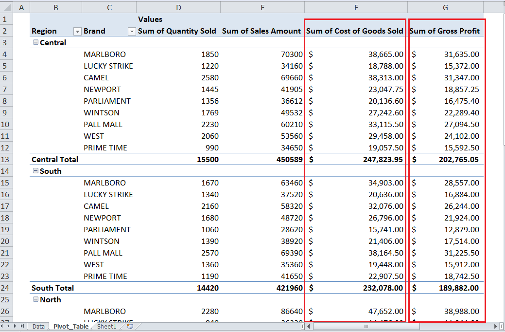
Using a Pivot table, you can easily summarize sales data of region and brand fields by quantity sold and sales amount by placing Region and Brand fields in Row area, and Quantity Sold and Sales Amount fields in Values area as shown below.
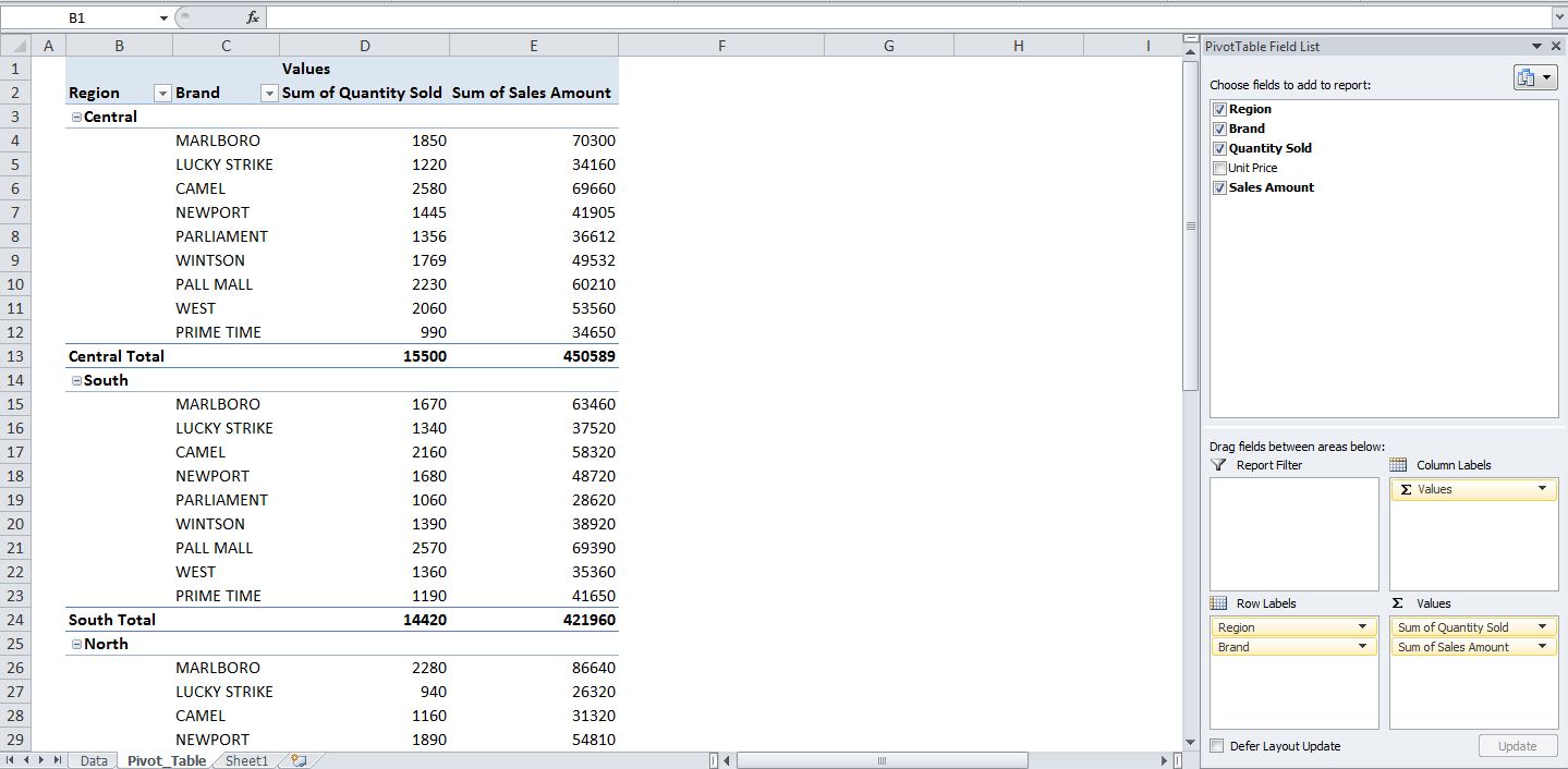
Now you want to calculate and summarize Cost of Goods Sold and Gross Profit in a Pivot table. In this example, you will learn how to create/add these new Calculated Fields by using the data of other fields in a Pivot table based on a formula.
You can calculate Cost of Goods Sold and Gross Profit by applying the following formulas;
Cost of Goods Sold= Sales Amount * 60%
You can calculate values of Cost of Goods Sold by multiplying values of Sales Amount field by a constant of 60%.
Gross Profit= Sales Amount – Cost of Goods Sold
You can calculate the values of Gross Profit field by subtracting the values of Cost of Goods Sold field from values of Sales Amount field.
How to create a Calculated Field in a Pivot Table
Now you will learn how to create these Calculated Fields one by one by following these steps. To insert a Calculated Field, execute the following steps.
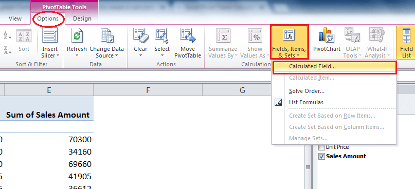
- Click any cell inside the pivot table.
- On Options or Analyze tab, in the Calculations group, click Fields, Items & Sets and click Calculated Field.
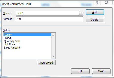
- The Insert Calculated Field dialog box appears.
- Enter Name of Calculated Field
- Type the formula
- Click Add button
- Click OK button
Now, by following the above steps, you will learn to create your desired two Calculated Fields as discussed above.
Cost of Goods Sold Calculated Field
This calculated field uses the following Pivot table field in the below formula;
Formula = ‘Sales Amount’ * 60%
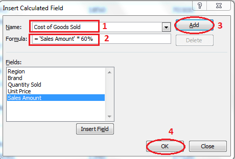
Excel automatically creates this Calculated Field and adds in Values area of Pivot Table Fields List panel. As this field contains numbers, so Pivot table by default SUM the values, as shown below;
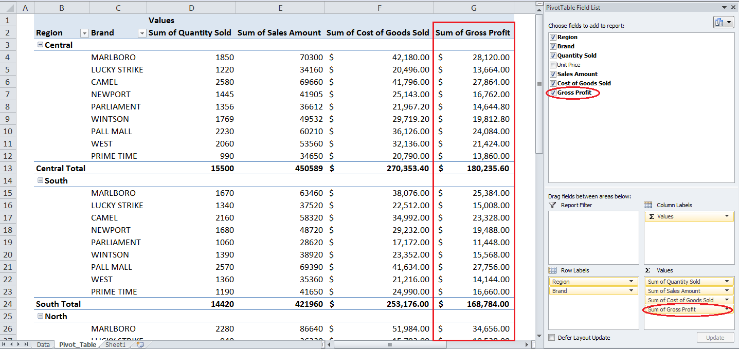
Gross Profit Calculated Field
This calculated field uses the following fields in the below formula;
Formula = ‘Sales Amount’ – ‘Cost of Goods Sold’
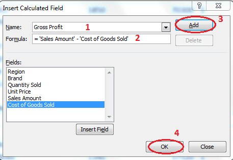
Calculated Field is created automatically and added to Pivot table Fields list’s Values area, and resulting values are summarized by SUM.
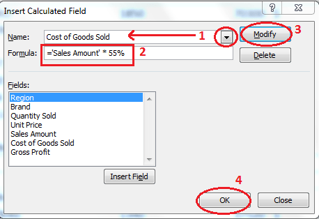
How to modify Calculated Fields in a Pivot Table
You can modify an existing Calculated Field by editing its formula in Insert Calculated Field dialog box by following these steps;
- Click drop down the list of Name, select Calculated Field name you want to modify
- Edit the formula
- Click on Modify button
- Click OK button
Now suppose you want to modify the Cost of Goods Sold calculated field by editing the percentage in formula from 60% to 55%. By following the above steps, you can modify this existing Calculated Field, and its values will be updated automatically. This change will show the impact on calculations of other Calculated Fields, where this Calculated Field is used, such as in Gross Profit.
How to delete a Calculated Fields in Pivot Table
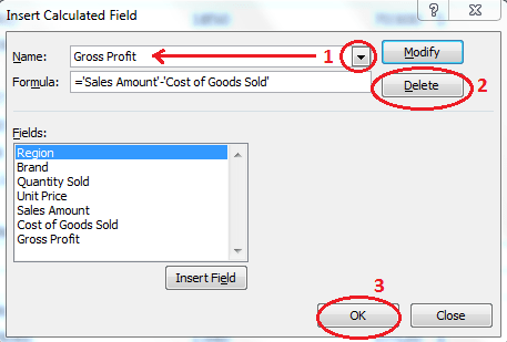
You can delete a Calculated Field from Pivot table by performing the following steps on Insert Calculated Field dialog box;
- Click drop down the list of Name, select Calculated Field name you want to delete
- Click on Delete button
- Click OK button
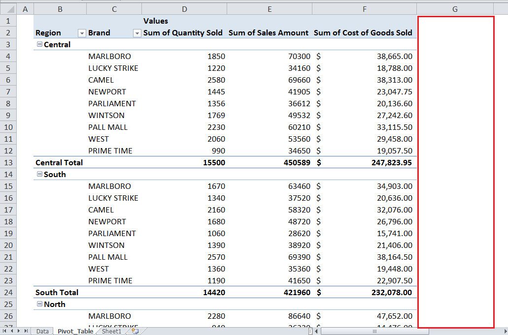
Suppose you want to delete Gross Profit Calculated Field from Pivot table, so you can do it by following the above steps, as shown below.
Still need some help with Excel formatting or have other questions about Excel? Connect with a live Excel expert here for some 1 on 1 help. Your first session is always free.