Calculated column in excel

Calculated columns in Excel tables are a fantastic tool for entering formulas efficiently. They allow you to enter a single formula in one cell, and then that formula will automatically expand to the rest of the column by itself. There’s no need to use the Fill or Copy commands. This can be incredibly time saving, especially if you have a lot of rows. And the same thing happens when you change a formula; the change will also expand to the rest of the calculated column.

Note: The screen shots in this article were taken in Excel 2016. If you have a different version your view might be slightly different, but unless otherwise noted, the functionality is the same.

Create a calculated column

1. Create a table. If you’re not familiar with Excel tables, you can learn more at: Overview of Excel tables.

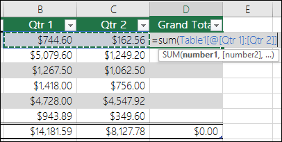
2. Insert a new column into the table. You can do this by typing in the column immediately to the right of the table, and Excel will automatically extend the table for you. In this example, we created a new column by typing «Grand Total» into cell D1.

   

   Tips: 

   • You can also add a table column from the Home tab. Just click on the arrow for Insert > Insert Table Columns to the Left.

   • 

3. Type the formula that you want to use, and press Enter.

   

   In this case we entered =sum(, then selected the Qtr 1 and Qtr 2 columns. As a result, Excel built the formula: =SUM(Table1[@[Qtr 1]:[Qtr 2]]). This is called a structured reference formula, which is unique to Excel tables. The structured reference format is what allows the table to use the same formula for each row. A regular Excel formula for this would be =SUM(B2:C2), which you would then need to copy or fill down to the rest of the cells in your column

   To learn more about structured references, see: Using structured references with Excel tables.

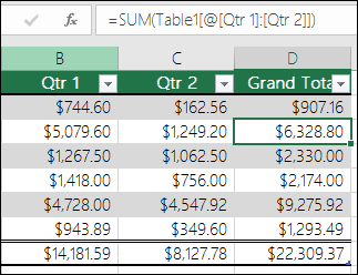
4. When you press Enter, the formula is automatically filled into all cells of the column — above as well as below the cell where you entered the formula. The formula is the same for each row, but since it’s a structured reference, Excel knows internally which row is which.

   

Notes: 

• Copying or filling a formula into all cells of a blank table column also creates a calculated column.

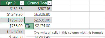
• If you type or move a formula in a table column that already contains data, a calculated column is not automatically created. However, the AutoCorrect Options button is displayed to provide you with the option to overwrite the data so that a calculated column can be created.

  

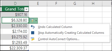
• If you input a new formula that is different from existing formulas in a calculated column, the column will automatically update with the new formula. You can choose to undo the update, and only keep the single new formula from the AutoCorrect Options button. This is generally not recommended though, because it can prevent your column from automatically updating in the future, since it won’t know which formula to extend when new rows are added.

  

• If you typed or copied a formula into a cell of a blank column and don’t want to keep the new calculated column, click Undo twice. You can also press Ctrl + Z twice

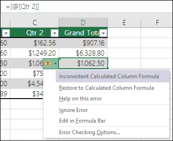
A calculated column can include a cell that has a different formula from the rest. This creates an exception that will be clearly marked in the table. This way, inadvertent inconsistencies can easily be detected and resolved.

Note: Calculated column exceptions are created when you do any of the following:

• Type data other than a formula in a calculated column cell.

• Type a formula in a calculated column cell, and then click Undo on the Quick Access Toolbar.

• Type a new formula in a calculated column that already contains one or more exceptions.

• Copy data into the calculated column that does not match the calculated column formula.

  Note: If the copied data contains a formula, this formula will overwrite the data in the calculated column.

• Delete a formula from one or more cells in the calculated column.

  Note: This exception is not marked.

• Move or delete a cell on another worksheet area that is referenced by one of the rows in a calculated column.

Error notification will only appear if you have the background error checking option enabled. If you don’t see the error, then go to File > Options > Formulas > make sure the Enable background error checking box is checked.

• If you’re using Excel 2007, click the Office button , then Excel Options > Formulas.

• If you’re using a Mac, go to Excel on the menu bar, and then click Preferences > Formulas & Lists > Error Checking.

The option to automatically fill formulas to create calculated columns in an Excel table is on by default. If you don’t want Excel to create calculated columns when you enter formulas in table columns, you can turn the option to fill formulas off. If you don’t want to turn the option off, but don’t always want to create calculated columns as you work in a table, you can stop calculated columns from being created automatically.

• Turn calculated columns on or off

  1. On the File tab, click Options.

     If you’re using Excel 2007, click the Office button , then Excel Options.

  2. Click Proofing.

  3. Under AutoCorrect options, click AutoCorrect Options.

  4. Click the AutoFormat As You Type tab.

  5. Under Automatically as you work, select or clear the Fill formulas in tables to create calculated columns check box to turn this option on or off.

     

     Tip: You can also click the AutoCorrect Options button that is displayed in the table column after you enter a formula. Click Control AutoCorrect Options, and then clear the Fill formulas in tables to create calculated columns check box to turn this option off.

  If you’re using a Mac, goto Excel on the main menu, then Preferences > Formulas and Lists > Tables & Filters > Automatically fill formulas.

• Stop creating calculated columns automatically

  After entering the first formula in a table column, click the AutoCorrect Options button that is displayed, and then click Stop Automatically Creating Calculated Columns.

You can also create custom calculated fields with PivotTables, where you create one formula and Excel then applies it to an entire column. Learn more about Calculating values in a PivotTable.

Need more help?

You can always ask an expert in the Excel Tech Community or get support in the Answers community.

See Also

Overview of Excel tables

Format an Excel table

Resize a table by adding or removing rows and columns

Total the data in an Excel table

Excel Tables are very useful in managing and analyzing data in tabular format. An Excel Table provides the data in a special structure, which comes with filtering, formatting, and sizing, and can also auto populate formulas dynamically. In this guide, we’re going to show you how to create calculated columns in Excel tables.

How to Create Calculated Columns in Excel Tables

Follow the steps below to add calculated columns into your Excel Tables. Since you want to add a formula, you may already have an Excel Table. If you don’t have your table yet, please see How to insert an Excel table for more details.

1.      Select a cell inside the column

Begin by selecting a cell inside the column you want to add your formulas. It doesn’t matter which row you click on, as long as it is not in the header row.

2.      Enter the formulas

Enter your formulas and press Enter to populate the entire column with your formula. Excel will automatically match the formatting, aggregate calculations, and add or remove any fields as necessary.

3.      (Optional) Update the header of the new column

If you add a brand new column without setting a header, Excel will give it a generic name like Column1. Simply click on the header cell and type in the header name you want. This step obviously won’t be necessary if you’re using an existing column for adding formulas.

4.      (Optional) Customization

You can now customize your table however you’d like. For more information, please see Tips for Excel Tables

In this article, we will learn How to Create Calculated Column(s) in Excel.

Scenario

If you want to get the sum of a column by just using the column name, you can do this in 3 easy ways in Excel. Let’s explore these ways.

Unlike other articles, let’s see with different scenarios first.

How to create a calculated column in a Table:

1. Select a cell in one of the columns of a Table or a blank cell right to the last column, in the example below the selected cell is G2.
2. Insert the formula that calculates sales per unit, type the equal (=) symbol, select cell F2, type the divide (/) symbol, and then select cell E2, and press Enter.

The formula is automatically copied to all the cells in the column.

Example :

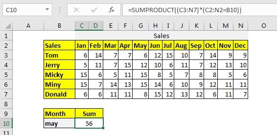
Here I have a table of sales done by different salesmen in different months.

Now the task is to get the sum of given month’s sales in Cell C10. If we change the month in B10, the sum should change and return that month’s sum, without changing anything in the formula.

Method 1: Sum Whole Column in Table Using SUMPRODUCT function.

The syntax of the SUMPRODUCT method to sum matching column is:

Columns: It is the 2-dimensional range of the columns that you want to sum. It should not contain headers. In the table above it is C3:N7.

Headers: It is the header range of columns that you want to sum. In the above data, it is C2:N2.

Heading: It is the heading that you want to match. In the example above, it is in B10.

Without further delay let’s use the formula.

and this will return:

How does it work?

It is simple. In the formula, the statement C2:N2=B10 returns an array that contains all FALSE values except one that matches B10. Now the formula is

=SUMPRODUCT((C3:N7)*{FALSE,FALSE,FALSE,FALSE,TRUE,FALSE,FALSE,FALSE,FALSE,FALSE,FALSE,FALSE})

Now C3:N7 is multiplied to each value of this array. Every column becomes zero except the column that is multiplied by TRUE. Now the formula becomes:

=SUMPRODUCT({0,0,0,0,6,0,0,0,0,0,0,0;0,0,0,0,12,0,0,0,0,0,0,0;0,0,0,0,15,0,0,0,0,0,0,0;0,0,0,0,15,0,0,0,0,0,0,0;0,0,0,0,8,0,0,0,0,0,0,0})

Now this array is summed up, and we get the sum of the column that matches the column in the cell B10.

Method 2: Sum Whole Column in Table Using INDEX-MATCH function.

The syntax of the method to sum the matching column heading in excel is:

All the variables in this method are the same as the SUMPRODUCT method. Let’s just implement it to solve the problem. Write this formula in C10.

This returns:

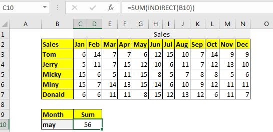
Method 3: Sum Whole Column in Table Using Named Range and INDIRECT function

Everything get’s simple if you name your ranges as column headings. In this method, we first need to name the columns as their heading names.

Select the table including the headings and press CTRL+SHIFT+F3. It will open a dialog to create a name from the ranges. Check the top row and hit the OK button.

It will name all the data columns as their headings.

Now the generic formula to sum the matching column will be:

Heading: It is the name of the column that you want to sum. In this example, it is B10 that contains may as of now.

To implement this generic formula, write this formula in cell C10.

This returns the sum of May month:

Another method is similar to this. In this method, we use excel tables and it’s structured naming. Let’s say if you have named the above table as table1. Then this formula will work the same as the above formula.

=SUM(INDIRECT(«Table1[«&B10&»]»))

Hope this article about How to Create Calculated Column(s) in Excel is explanatory. Find more articles on calculating values and related Excel formulas here. If you liked our blogs, share it with your friends on Facebook. And also you can follow us on Twitter and Facebook. We would love to hear from you, do let us know how we can improve, complement or innovate our work and make it better for you. Write to us at info@exceltip.com.

Related Articles :

How to Sum by Matching Row and Column in Excel : The SUMPRODUCT is the most versatile function when it comes to sum and count values with tricky criteria. The generic function to sum by matching column and row is…

SUMIF with 3D Reference in Excel : The fun fact is that the normal Excel 3D referencing does not work with conditional functions, like SUMIF function. In this article, we will learn how to get 3D referencing working with SUMIF function.

Relative and Absolute Reference in Excel : Referencing in excel is an important topic for every beginner. Even experienced excel users make mistakes in referencing.

Dynamic Worksheet Reference : Give reference sheets dynamically using the INDIRECT function of excel. This is simple…

Expanding References in Excel : The expanding reference expands when copied down or rightwards. We use the $ sign before the column and row number to do so. Here is one example…

All About Absolute Reference : The default reference type in excel is relative but if you want the reference of cells and ranges to be absolute use the $ sign. Here are all the aspects of absolute referencing in Excel.

Popular Articles :

How to use the IF Function in Excel : The IF statement in Excel checks the condition and returns a specific value if the condition is TRUE or returns another specific value if FALSE.

How to use the VLOOKUP Function in Excel : This is one of the most used and popular functions of excel that is used to lookup value from different ranges and sheets.

How to use the SUMIF Function in Excel : This is another dashboard essential function. This helps you sum up values on specific conditions.

How to use the COUNTIF Function in Excel : Count values with conditions using this amazing function. You don’t need to filter your data to count specific values. Countif function is essential to prepare your dashboard.

---

A calculated column is a column that you add to an existing table in the Data Model of your workbook by means of a DAX formula that defines the column values. Instead of importing the values in the column, you create the calculated column.

You can use the calculated column in a PivotTable, PivotChart, Power PivotTable, Power PivotChart or Power View report just like any other table column.

Understanding Calculated Columns

The DAX formula used to create a calculated column is like an Excel formula. However, in DAX formula, you cannot create different formulas for different rows in a table. The DAX formula is automatically applied to the entire column.

For example, you can create one calculated column to extract Year from the existing column – Date, with the DAX formula −

= YEAR ([Date]) 

YEAR is a DAX function and Date is an existing column in the table. As seen, the table name is enclosed in brackets. You will learn more about this in the chapter – DAX Syntax.

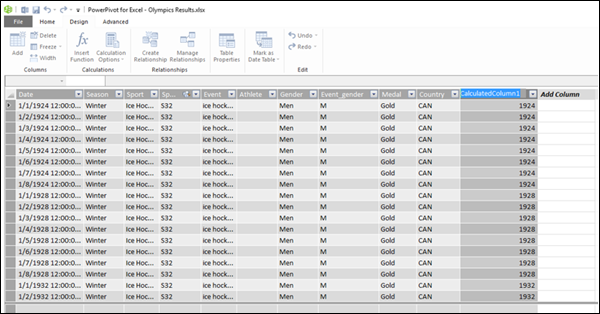
When you add a column to a table with this DAX formula, the column values are computed as soon as you create the formula. A new column with the header CalculatedColumn1 filled with Year values will get created.

Column values are recalculated as necessary, such as when the underlying data is refreshed. You can create calculated columns based on existing columns, calculated fields (measures), and other calculated columns.

Creating a Calculated Column

Consider the Data Model with the Olympics Results as shown in the following screenshot.

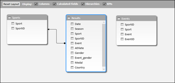
• Click the Data View.
• Click the Results tab.

You will be viewing the Results table.

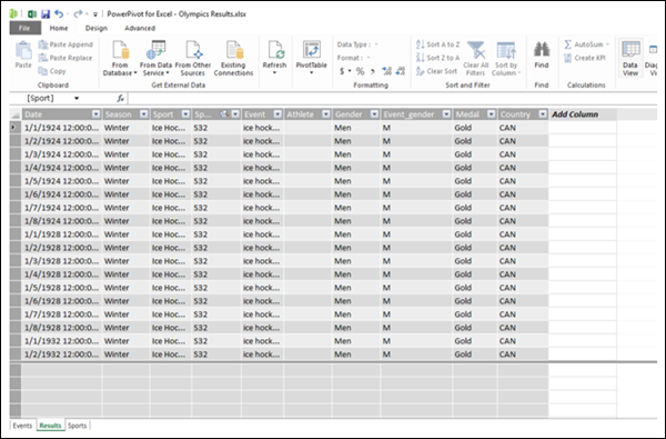
As seen in the above screenshot, the rightmost column has the header – Add Column.

• Click the Design tab on the Ribbon.
• Click Add in the Columns group.

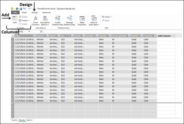
The pointer will appear in the formula bar. That means you are adding a column with a DAX formula.

• Type =YEAR ([Date]) in the formula bar.

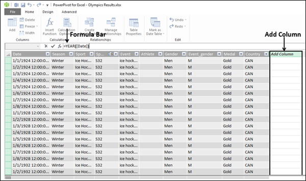
As can be seen in the above screenshot, the rightmost column with the header – Add Column is highlighted.

• Press Enter.

It will take a while (few seconds) for the calculations to be done. Please wait.

The new calculated column will get inserted to the left of the rightmost Add Column.

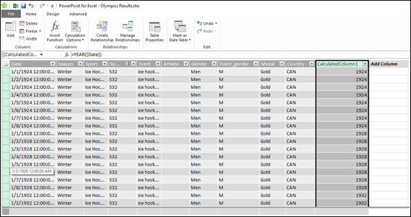
As shown in the above screenshot, the newly inserted calculated column is highlighted. Values in the entire column appear as per the DAX formula used. The column header is CalculatedColumn1.

Renaming the Calculated Column

To rename the calculated column to a meaningful name, do the following −

• Double-click on the column header. The column name will be highlighted.

• Select the column name.
• Type Year (the new name).

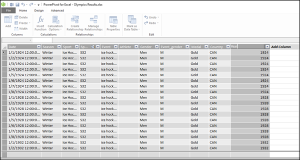
As seen in the above screenshot, the name of the calculated column got changed.

You can also rename a calculated column by right-clicking on the column and then clicking on Rename in the dropdown list.

Just make sure that the new name does not conflict with an existing name in the table.

Checking the Data Type of the Calculated Column

You can check the data type of the calculated column as follows −

• Click the Home tab on the Ribbon.
• Click the Data Type.

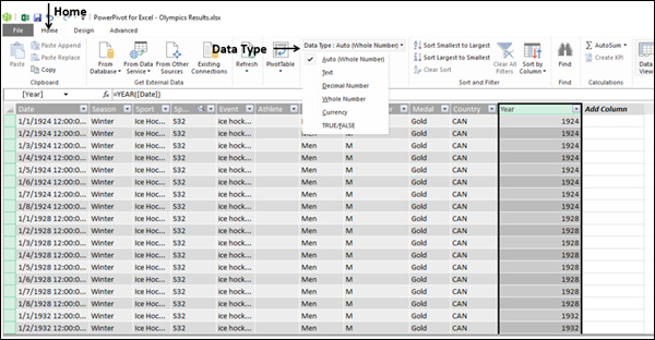
As you can see in the above screenshot, the dropdown list has the possible data types for the columns. In this example, the default (Auto) data type, i.e. the Whole Number is selected.

Errors in Calculated Columns

Errors can occur in the calculated columns for the following reasons −

• Changing or deleting relationships between the tables. This is because the formulas that use columns in those tables will become invalid.

• The formula contains a circular or self-referencing dependency.

Performance Issues

As seen earlier in the example of Olympics results, the Results table has about 35000 rows of data. Hence, when you created a column with a DAX formula, it had calculated all the 35000+ values in the column at once, for which it took a little while. The Data Model and the tables are meant to handle millions of rows of data. Hence, it can affect the performance when the DAX formula has too many references. You can avoid the performance issues doing the following −

• If your DAX formula contains many complex dependencies, then create it in steps saving the results in new calculated columns, instead of creating a single big formula at once. This enables you to validate the results and assess the performance.

• Calculated columns need to be recalculated when data modifications occur. You can set the recalculation mode to manual, thus saving frequent recalculations. However, if any values in the calculated column are incorrect, the column will be grayed out, until you refresh and recalculate the data.