Calculate total in excel

SUM function

The SUM function adds values. You can add individual values, cell references or ranges or a mix of all three.

For example:

=SUM(A2:A10) Adds the values in cells A2:10.
=SUM(A2:A10, C2:C10) Adds the values in cells A2:10, as well as cells C2:C10.

SUM(number1,[number2],…)

Argument name	Description
number1 Required	The first number you want to add. The number can be like 4, a cell reference like B6, or a cell range like B2:B8.
number2-255 Optional	This is the second number you want to add. You can specify up to 255 numbers in this way.

Argument name

Description

number1

Required

The first number you want to add. The number can be like 4, a cell reference like B6, or a cell range like B2:B8.

number2-255

Optional

This is the second number you want to add. You can specify up to 255 numbers in this way.

This section will discuss some best practices for working with the SUM function. Much of this can be applied to working with other functions as well.

The =1+2 or =A+B Method – While you can enter =1+2+3 or =A1+B1+C2 and get fully accurate results, these methods are error prone for several reasons:

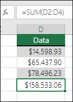
Typos – Imagine trying to enter more and/or much larger values like this:
- =14598.93+65437.90+78496.23
Then try to validate that your entries are correct. It’s much easier to put these values in individual cells and use a SUM formula. In addition, you can format the values when they’re in cells, making them much more readable then when they’re in a formula.
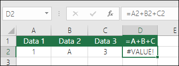
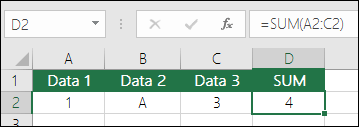
#VALUE! errors from referencing text instead of numbers

If you use a formula like:
- =A1+B1+C1 or =A1+A2+A3
Your formula can break if there are any non-numeric (text) values in the referenced cells, which will return a #VALUE! error. SUM will ignore text values and give you the sum of just the numeric values.
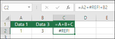
#REF! error from deleting rows or columns

If you delete a row or column, the formula will not update to exclude the deleted row and it will return a #REF! error, where a SUM function will automatically update.
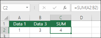
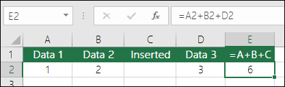
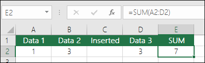
Formulas won’t update references when inserting rows or columns

If you insert a row or column, the formula will not update to include the added row, where a SUM function will automatically update (as long as you’re not outside of the range referenced in the formula). This is especially important if you expect your formula to update and it doesn’t, as it will leave you with incomplete results that you might not catch.
SUM with individual Cell References vs. Ranges

Using a formula like:
- =SUM(A1,A2,A3,B1,B2,B3)
Is equally error prone when inserting or deleting rows within the referenced range for the same reasons. It’s much better to use individual ranges, like:
- =SUM(A1:A3,B1:B3)
Which will update when adding or deleting rows.

I just want to Add/Subtract/Multiply/Divide numbers See this video series on Basic Math in Excel, or Use Excel as your calculator.
How do I show more/less decimal places? You can change your number format. Select the cell or range in question and use Ctrl+1 to bring up the Format Cells Dialog, then click the Number tab and select the format you want, making sure to indicate the number of decimal places you want.
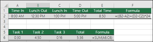
How do I add or subtract Times? You can add and subtract times in a few different ways. For example, to get the difference between 8:00 AM — 12:00 PM for payroll purposes you would use: =(«12:00 PM»-«8:00 AM»)*24, taking the end time minus the start time. Note that Excel calculates times as a fraction of a day, so you need to multiply by 24 to get the total hours. In the first example we’re using =((B2-A2)+(D2-C2))*24 to get the sum of hours from start to finish, less a lunch break (8.50 hours total).

If you’re simply adding hours and minutes and want to display that way, then you can sum and don’t need to multiply by 24, so in the second example we’re using =SUM(A6:C6) since we just need the total number of hours and minutes for assigned tasks (5:36, or 5 hours, 36 minutes).

For more information, see: Add or subtract time.
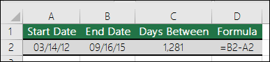
How do I get the difference between dates? As with times, you can add and subtract dates. Here’s a very common example of counting the number of days between two dates. It’s as simple as =B2-A2. The key to working with both Dates and Times is that you start with the End Date/Time and subtract the Start Date/Time.

For more ways to work with dates see: Calculate the difference between two dates.
How do I sum just visible cells? Sometimes, when you manually hide rows or use AutoFilter to display only certain data you also only want to sum the visible cells. You can use the SUBTOTAL function. If you’re using a total row in an Excel table, any function you select from the Total drop-down will automatically be entered as a subtotal. See more about how to Total the data in an Excel table.

Need more help?

You can always ask an expert in the Excel Tech Community or get support in the Answers community.

Calculating Running Total with Tabular Data

If you have tabular data (i.e., a table in Excel which is not converted into an Excel table), you can use some simple formulas to calculate the running totals.

Using the Addition Operator

Suppose you have date-wise sales data and you want to calculate the running total in column C.

Below are the steps to do this.

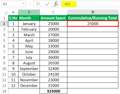
Step 1 – In cell C2, which is the first cell where you want the running total, enter

=B2

This will simply get the same sale values in cell B2.

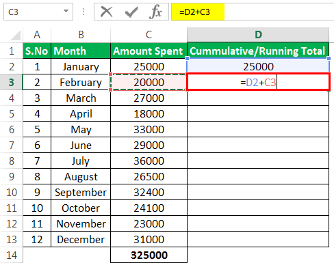
Step 2 – In cell C3, enter the below formula:

=C2+B3

Step 3 – Apply the formula to the entire column. You can use the Fill handle to select and drag it, or simply and copy-paste the cell C3 to all the remaining cells (which would automatically adjust the reference and give the right result).

This will give you the result as shown below.

It’s a really simple method and works well in most cases.

The logic is simple – every cell picks up the value above it (which is the cumulative sum till the date before) and adds the value in the cell adjacent to it (which is the sale value for that day).

There is only one drawback – in case you delete any of the existing rows in this data set, all the cells below that would return a reference error (#REF!)

If that’s a possibility with your data set, use the next method that uses the SUM formula

Using SUM with Partially Locked Cell Reference

Suppose you have date-wise sales data and you want to calculate the running total in column C.

Below is the SUM formula that will give you the running total.

=SUM($B$2:B2)

Let me explain how this formula works.

In the above SUM formula, I have used the reference to add as $B$2:B2

$B$2 – this is an absolute reference, which means that when I copy the same formula in the cells below, this reference is not going to change. So when copying the formula in the cell below, the formula would change to SUM($B$2:B3)
B2 – this is the second part of the reference which is a relative reference, which means that this would adjust as I copy the formula down or to the right. So when copying the formula in the cell below, this value will become B3

Also read: Absolute, Relative, and Mixed Cell References in Excel

The great thing about this method is that in case you delete any of the rows in the data set, this formula would adjust and still give you the right running totals.

Calculating Running Total in Excel Table

When working with tabular data in Excel it’s a good idea to convert it into an Excel table. It makes it a lot easier to manage the data and also allows makes it easy to use tools such as Power Query and Power Pivot.

Working the Excel tables comes with benefits such as structured references (which makes it really easy to refer to the data in the table and use it in formulas), and automatic adjustment of references in case you add or delete data from the table.

While you can still use the above formula that I have shown you in an Excel table, let me show you some better methods to do this.

Suppose you have an Excel table as shown below and you want to calculate the running total in column C.

Below is the formula that will do this:

=SUM(SalesData[[#Headers],[Sale]]:[@Sale])

The above formula may look a bit long, but you don’t have to write it yourself. what you see within the sum formula are called structured references, which is Excel’s efficient way to refer to specific data points in an Excel table.

For example, SalesData[[#Headers],[Sale]] refers to the Sale header in the SalesData table (SalesData is the name of the Excel table that I gave when I created the table)

And [@Sale] refers to the value in the cell in the same row in the Sale column.

I just explained this here for your understanding, but even if you know nothing about structured references, you can still easily create this formula.

Below are the steps to do this:

In cell C2, enter =SUM(
Select cell B1, which is the header of the column that has the sale value. You can use the mouse or use the arrow keys. You will notice that Excel automatically enters the structured reference for that cell
Add a : (colon symbol)
Select cell B2. Excel would again automatically insert the structured reference for the cell
Close the bracket and hit enter

You will also notice that you don’t have to copy the formula in the entire column, an Excel table automatically does it for you.

Another great thing about this method is that in case you add a new record in this data set, the Excel table would automatically calculate the running total for all the new records.

While we have included the header of the column in our formula, remember that the formula would ignore the header text and only consider the data in the column

Calculating Running Total Using Power Query

Power Query is an amazing tool when it comes to connecting with databases, extracting the data from multiple sources, and transforming it before putting it into Excel.

If you are already working with Power Query, it would be more efficient to add running totals while you are transforming the data within the Power Query editor itself (instead of 1st getting the data in Excel and then adding the running totals using any of the above methods covered above).

While there is no inbuilt feature in Power Query to add running totals (which I wish there was), you can still do that using a simple formula.

Suppose you have an Excel table as shown below and you want to add the running totals to this data:

Below are the steps to do this:

Select any cell in the Excel table
Click on Data
In the Get & Transform tab, click on the from Table/Range icon. This will open the table in the Power Query editor
[Optional] In case your Date column is not already sorted, click on the filter icon in the Date column, and then click on Sort ascending
Click the Add Column tab in the Power Query editor
In the General group, click on the Index Column dropdown (do not click on the Index Column icon, but on the small black tilted arrow right next to it to show more options)
Click on the ‘From 1’ option. Doing this will add a new index column that would start from one and enter numbers incrementing by 1 in the entire column
Click on the ‘Custom Column’ icon (which is also in the Add Column tab)
In the custom column dialog box that opens up, enter a name for the new column. in this example, I will use the name ‘Running Total’
In the Custom column formula field, enter the below formula: List.Sum(List.Range(#”Added Index”[Sale],0,[Index]))
Make sure there’s a checkbox at the bottom of the dialog box that says – ‘No syntax errors have been detected’
Click OK. This would add a new running total column
Remove the Index Column
Click on the File tab and then click on ‘Close and Load’

The above steps would insert a new sheet in your workbook with a table that has the running totals.

Now if you’re thinking that these are just too many steps as compared to the previous methods of using simple formulas, you’re right.

If you already have a data set and all you need to do is add running totals, it’s better not to use Power Query.

Using Power Query makes sense where you have to extract data from a database or combine data from multiple different workbooks and in the process also add running totals to it.

Also, once you do this automation using Power Query, the next time your data set changes you do not have to do it again you can simply refresh the query and it would give you the result based on the new data set.

How does this work?

Now let me quickly explain what happens in this method.

The first thing we do in the Power Query editor is to insert an index column starting from one and incrementing by one as it goes down the cells.

We do this because we need to use this column while we calculate the running total in another column that we insert in the next step.

Then we insert a custom column and use the below formula

List.Sum(List.Range(#"Added Index"[Sale],0,[Index]))

This is a List.Sum formula that would give you the sum of the range that is specified within it.

And that range is specified using the List.Range function.

The List.Range function gives the specified range in the sale column as the output and this range changes based on the Index value. For example, for the first record, the range would simply be the first sale value. And as you go down the cells, this range would expand.

So, for the first cell. List.Sum would only give you the sum of the first sale value, and for the second cell, it would give you the sum for the first two sale values and so on.

While this method works well, gets really slow with large datasets – thousands of rows. If you’re dealing with a large data set and want to add running totals to it, have a look at this tutorial that shows other methods that are faster.

Calculating Running Total Based on Criteria

So far, we have seen examples where we have calculated the running total for all the values in a column.

But there could be cases where you want to calculate the running total for specific records.

For example, below I have a data set and I want to calculate the running total for Printers and Scanners separately in two different columns.

This can be done using a SUMIF formula that calculates the running total while making sure the specified condition is met.

Below is the formula that will do this for the Printer columns:

=SUMIF($C$2:C2,$D$1,$B$2:B2)

Similarly, to calculate the running total for Scanners, use the below formula:

=SUMIF($C$2:C2,$E$1,$B$2:B2)

In the above formulas, I have used SUMIF, which would give me the sum in a range when the specified criteria are met.

The formula takes three arguments:

range: this is the criteria range that would be checked against the specified criteria
criteria: this is the criteria that would be checked in only if this criterion is met then the values in the third argument, which is the sum range, would be added
[sum_range]: this is the sum range from which the values would be added if the criteria are met

Also, in the range and sum_range argument, I have locked the second part of the reference, so that as we go down the cells, the range would keep expanding. This allows us to only consider and add values till that range (hence running totals).

In this formula, I have used the header column (Printer and Scanner) as the criteria. you can also hardcode the criteria if your column headers are not exactly the same as the criteria text.

In case you have multiple conditions that you need to check, then you can use the SUMIFS formula.

Running Total in Pivot Tables

If you want to add running totals in a Pivot Table result, you can easily do that using an inbuilt functionality in Pivot tables.

Suppose you have a Pivot Table as shown below where I have the date in one column and the sale value in the other column.

Below are the steps to add an additional column that will show the running total of the sales by date:

Drag the Sale field and put it in the Value area.
This will add another column with the Sales values
Click on the Sum of Sale2 option in the Value area
Click on the ‘Value Field Settings’ option
In the Value Field Settings dialog box, change the Custom Name to ‘Running Totals’
Click on the ‘Show Value As’ tab
In the Show value as drop-down, select the ‘Running Total in’ option
In the Base field options, make sure Date is selected
Click Ok

The above steps would change the second sale column into the Running Total column.

So these are some of the ways you can use to calculate the running total in Excel. If you have data in tabular format, you can use simple formulas, and if you have an Excel table, then you can use formulas that make use of structured references.

I’ve also covered how to calculate running total using Power Query and in Pivot Tables.

I hope you found this tutorial useful.

Other Excel tutorials you may also like:

How to Sum a Column in Excel
Calculating Moving Average in Excel [Simple, Weighted, & Exponential]
Excel Quick Analysis Tool – How to Best Use it? 10 Examples!

Источник

A running total in Excel, also called “cumulative sum,” is the summation of numbers increasing or growing in quantity, degree, or force by successive additions. It is the total that gets updated when there is a new entry in the data. In Excel, the normal function to calculate the total is the SUM function, so if we have to calculate the running total to see how the data changes with every new entry, then the first-row reference will be absolute. In contrast, others change, calculating the running total in Excel.

Excel Running Total
- How to Calculate Running Total (Cumulative Sum) in Excel?
  - Example #1 – Performing “Running Total or Cumulative” with Simple Formula
  - Example #2 – Performing “Running Total or Cumulative” with “SUM” Formula
  - Example #3 – Performing “Running Total or Cumulative” with a Pivot Table
  - Example #4 – Performing “Running Total or Cumulative” with a Relative Named Range
- Things to Remember
- Recommended Articles

How to Calculate Running Total (Cumulative Sum) in Excel?

You can download this Running Total Calculation Excel Template here – Running Total Calculation Excel Template

Example #1 – Performing “Running Total or Cumulative” with Simple Formula

Let us start.

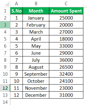
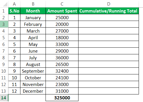
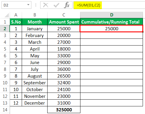
Let us assume that we have the data on our expenses every month as follows:
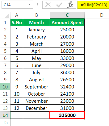
From this data, we can observe that we spent 3,25,000 in total from January to December.
Now, let us see how much of my total expenses were made by the end of the month. We will use a simple formula in Excel to calculate as required.
First, we should consider the amount spent in a particular month, January, as we contemplate our spent calculation from January.
Now, calculate the money spent for the rest of the months as follows:

February – D2+C3
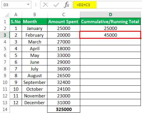
The running total for February month is 45,000.

For the next month onwards we have to consider the money spent till the previous month and money spent in the current month:

March – C4+D3
Similarly, for the rest of the months, the result would be as follows:

From the above result, we can observe that by the end of the year in December, we had spent 3,25,000, which is the total amount from the start of the year. Therefore, this running total will tell us how much we had spent on a particular month.
Until July, we had spent 1,88,000. Till November, we had spent 2,94,000.

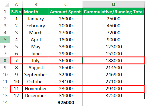
We can also use this data (running total) for certain analyses.

Q1) If we want to know by which month we had spent 90,000?

A) April – We can see the “Cumulative/Running Total” column from the table. It shows that the cumulative spending till April month is 90,000.

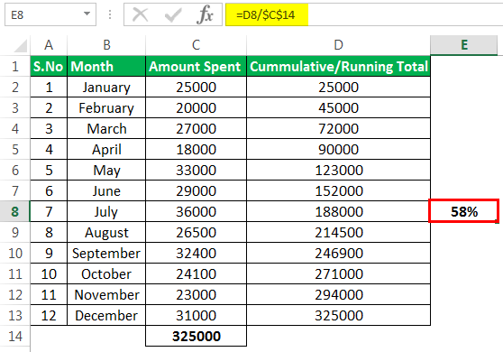
Q2) Suppose we want to know the % of money spent that we had spent till July?

A) 58% – We can take the amount spent till July and divide it by the total amount spent as follows.

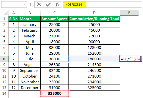
We had spent 58% of the money until July.

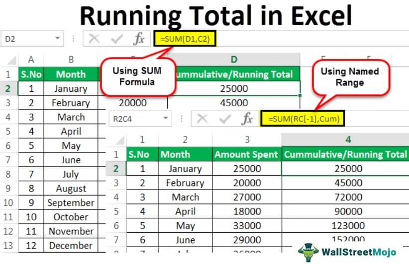
Example #2 – Performing “Running Total or Cumulative” with “SUM” Formula

In this example, we will use the SUM in excelThe SUM function in excel adds the numerical values in a range of cells. Being categorized under the Math and Trigonometry function, it is entered by typing “=SUM” followed by the values to be summed. The values supplied to the function can be numbers, cell references or ranges.read more instead of the “+” operator to calculate the cumulative in Excel.

But, first, apply the SUM Formula in excel.

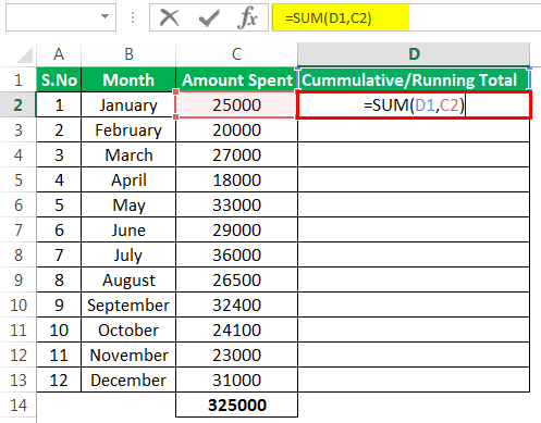
While using the SUM function, we should consider summing the earlier month spent and the current month spent. But for the first month, we should add earlier cells, i.e.cumulative, which will be regarded as zero.

Then, drag the formula to other cells.

Example #3 – Performing “Running Total or Cumulative” with a PivotTable

To perform running total using a PivotTable in Excel, we should create a PivotTable first. Create a pivot tableA Pivot Table is an Excel tool that allows you to extract data in a preferred format (dashboard/reports) from large data sets contained within a worksheet. It can summarize, sort, group, and reorganize data, as well as execute other complex calculations on it.read more by selecting the table and clicking on the PivotTable from the “Insert” tab.

We can see the PivotTable is created now. Drag the “Month” column into the “Rows” field and the “Amount Spent” column into the “Values” field. The table would be as follows:

Again, drag the “Amount Spent” column into the “Values” field to create a total running value. Then, right-click on the column as follows:

Click on “Show Value As,” and you will get an option of “Running Total In.”

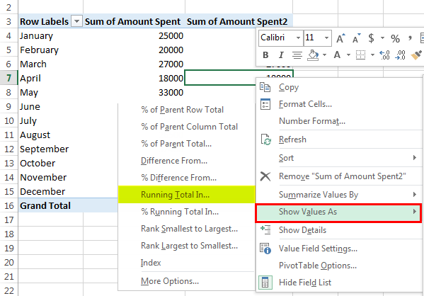
Now, we can see the table with a column having cumulative values as follows:

We can change the table’s name by editing the cell with a “Sum of Amount Spent2.”

Example #4 – Performing “Running Total or Cumulative” with a Relative Named Range

We need to make temporary changes in the Excel options to perform running total with a relative named range.

Change Excel referenceCell reference in excel is referring the other cells to a cell to use its values or properties. For instance, if we have data in cell A2 and want to use that in cell A1, use =A2 in cell A1, and this will copy the A2 value in A1.read more style from A1 to R1C1 from Excel options as below:

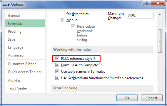
“Reference style R1C1” refers to “Row 1” and “Column 1.” This style can find positive and negative signs used for a reason.

In Rows: –

The +(positive) sign refers to a “Downward” direction.
The – (negative) sign refers to an “Upward” direction.

Ex- R[3] connects the cell 3 rows below the current cell. R[-5] connects the cell 5 rows above the current cell

In Columns: –

The +(positive) sign refers to the “Right” direction.
The – (negative) sign refers to the “Left” direction.

Ex- C[2] refers to connecting the cell, which is 2 columns right to the current cell, and C[-4] refers to connecting the cell, which is 4 columns left to the current cell.

To use the reference style to calculate the running total, we must define a name with certain criteria.

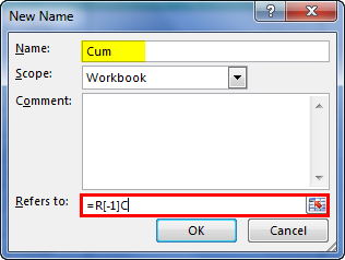
In our example, we have to define the name by “R[-1]C” because we are calculating the cumulative sum of the cell’s previous row and column with every month’s expense. Define a name in Excel with “Cum”(You can define it as per your wish) as follows:

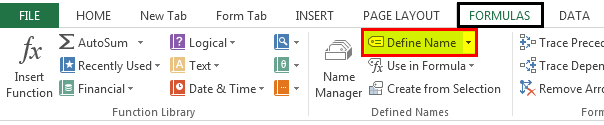
Go to the “Formulas” tab and select the “Define Name.”

Then, the “New Name” window will pop out and give the name per your wish and the condition you want to perform for the name you defined. Here, we take R[-1]C because we will sum the previous row of the cell and column with every month’s expense.

Once the name is defined, then go to the column of “Cumulative/Running Total” and use the defined name in the SUM function as follows:

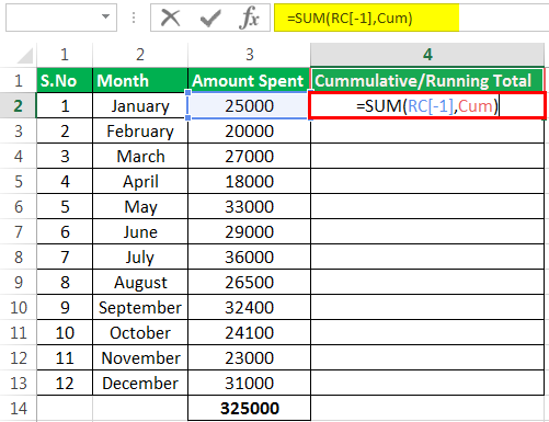
It tells us to perform SUM with the cell “RC[-1}” and “Cum” (Which is already defined), and in the first cell, we get the same expense incurred in January.

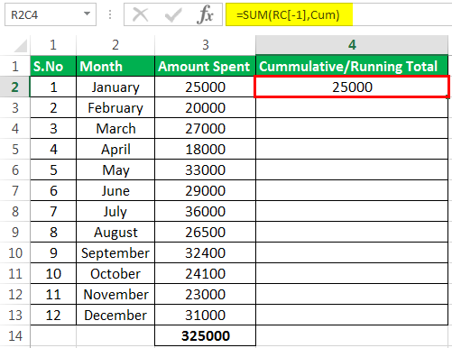
Then, drag down the formula to the end of the table. We can see the cumulative results will be out as below:

Things to Remember

The running total/cumulative will help analyze the data’s information for decision-making purposes.
A relatively named range running total is performed to avoid the problems with inserting and deleting rows from the data. This operation will refer to the cell as per the condition given though we insert or delete rows or columns.
Cumulative in Excel is mostly used in financial modelingFinancial modeling refers to the use of excel-based models to reflect a company’s projected financial performance. Such models represent the financial situation by taking into account risks and future assumptions, which are critical for making significant decisions in the future, such as raising capital or valuing a business, and interpreting their impact.read more, and the final cumulative value will be the same as the “Total Sum.”
The “Total Sum” and “Running Total” are different. The key difference is the computation we do. The “Total Sum” will perform the sum of each number in the data series. At the same time, the “Running Total” will sum the previous value with the current value from the data.

Video Tutorial

Watch on Youtube & Subscribe to our Channel

Download the Excel File

You can download the Excel file to follow along and practice writing your own formulas for running totals.

Paul, a member of our Elevate Excel Training Program, posted a great question in the Community Forum. He wanted to know the best way to create running totals in Excel Tables, since there are multiple ways to go about it.

The running total calculation sums all of the values in a column from the current row the formula is in to the first row in the data set.

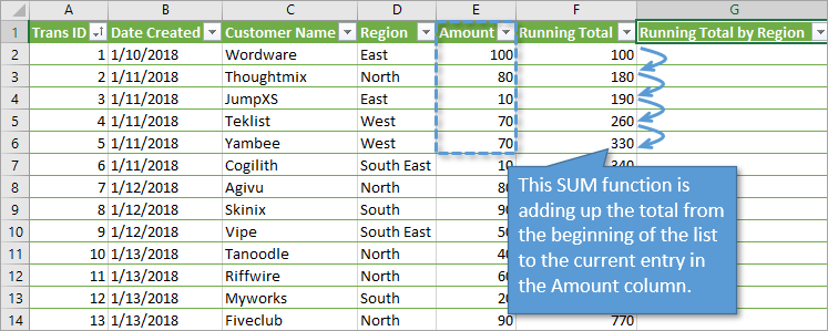
Therefore, we need to create a range reference that always starts at the first row in the column, down to the current row the formula is in.

When using Excel Tables, it’s best to use structured references (references to the table and column names) for running totals. Using regular cell references like ($A$2:A3) can cause errors in your formulas, more on that below.

Unfortunately, there is no straightforward way to create this reference with Table formulas. There are still many ways to solve this problem and I’ll share three methods in this post.

Method #1: Reference the Header Cell

My preferred method is to reference the header cell to create the absolute reference for the first cell in the range. Then reference the cell in the row that the formula is in for the last cell in the range. Here is an example.

=SUM(tblSales[[#Headers],[Amount]]:[@Amount]])

The reason I reference the header cell (tblSales[[#Headers],[Amount]]) is because the reference will NOT change as the formula is copied down. This makes it an absolute reference.

The ending reference [@Amount] creates a relative reference to the row that the formula is in.

In everyday terms, you’ve just told Excel to add up everything from the beginning of the Amount column (including the header row) down to the row the formula is in, and to return that value in the Running Total column.

Because we are using an Excel Table, the formula will automatically be copied down the entire column. You can see how each cell adds the current amount to the existing total to give a running total.

Tips for Writing the Formula

When writing this formula you can click the header cell to create the reference (tblSales[[#Headers],[Amount]]). You do NOT have to type out the entire reference.
After clicking the header cell, click into the end of the formula to edit it and type a : colon. Then select the cell in the row the formula is in to create the ending reference [@Amount].

A Few Notes About the References

There are a few good things to know about this running total formula with structured references.

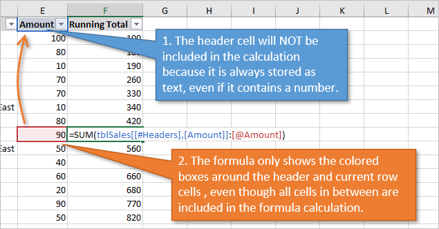
The header cell always contains the text data type. Therefore, the value in the header cell is NOT included in the SUM formula calculation. Even if the header cell contains a number, that number is stored as text and will not be included in the calculation.
When looking at the formula in Edit mode, only the cells in the header row and current row are selected. Excel does put a colored border around the entire range. This does not impact the results of the formula. All of the cells between the header cell and current row are included in the calculation. It is just a visual nuance to be aware of.

Why Use Structured References?

You may be wondering why I use structured references (tblSales[[#Headers],[Amount]]:[@Amount]]) instead of regular range references ($A$2:A2) in the SUM formula.

A formula with regular range references is probably easier to create and read in this scenario. However, the formulas don’t always get copied down properly. If you add new rows to the bottom of the table, the running total formula will not create a relative reference to the row the formula is in. Instead, it will likely keep a reference to the last row in the table BEFORE rows were added. This leaves us with incorrect results.

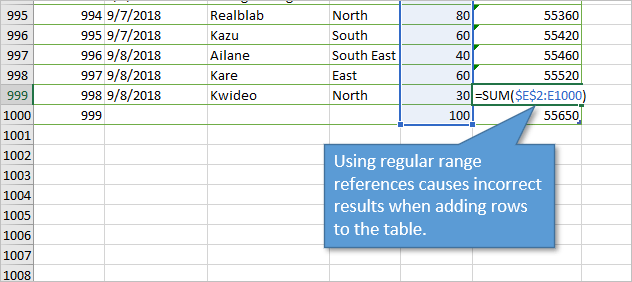
This happens because Excel remembers ONE formula for the entire column and copies it down. When using structured references, the formula text is the SAME in every cell of the running total column. Every cell contains: =SUM(tblSales[[#Headers],[Amount]]:[@Amount]])

Method #2: Mixed References

Another option is to create an absolute reference to the first cell in the column, combined with a structured reference for the last cell.

=SUM($E$2:[@Amount])

This method seems to work as well as the referencing the header row. I believe I’ve had issues with it in older versions of Excel, but can’t seem to break it in the current version of Microsoft 365. Therefore, my preference is to use full structured references.

Please leave a comment below if you use this method and/or have issues with it.

Method #3: SUM & INDEX

Another popular alternative uses the INDEX function within SUM.

=SUM(INDEX([Amount],1):[@Amount])

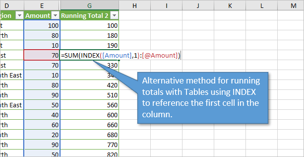
The INDEX function is used to create a reference to the first cell in the column because we reference a 1 for the row_num argument. INDEX([Amount],1)

This method works just as well, but there are two drawbacks that make me not love it as much:

The formula is more difficult to read and understand for users of your file that are not familiar with the INDEX function.
The entire column is referenced in the array argument of INDEX. This creates a colored border around the entire column when in formula edit mode, even though the function evaluates to create a reference to just the first cell. To me, this is a bit more confusing than the reference the to first and current cells that the first method uses.

Which Method is Best?

Honestly, none of these solutions are perfect. Each has their pros & cons. I just find method #1 easier to read, write, and understand.

It would be great if structured references had a better way to reference other cells in the column like the first cell, last cell, cell above, cell below, etc. I know we can create these with nested functions, but it makes it more challenging for other users of our files to understand.

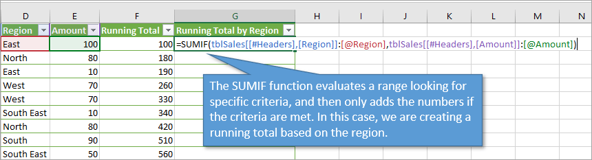
Running Total with Conditions

We can also use these any of these running range references in the SUMIF(S) function to create running totals based on a condition or criteria. In this example I create a running total by region. Here is an example of the formula.

=SUMIF(tblSales[[#Headers],[Region]]:[@Region],[@Region],tblSales[[#Headers],[Amount]]:[@Amount])

Click to enlarge

Here is an explanation of each component of the formula:

The first argument in SUMIF is the range we want to evaluate (tblSales[[#Headers],[Region]]:[@Region]). This uses the same running range reference method.
The second argument is the criteria or condition that we want to filter the range for ([@Region]). This is the value in the same row the formula is in from the Region column.
The third argument is the sum range which contains the values we want to sum with the criteria is True (tblSales[[#Headers],[Amount]]:[@Amount]).

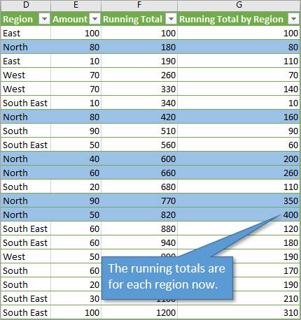
Now the running total column reflects running totals for each region. I’ve highlighted one of the regions (North) in the image below so you can see how the running totals are region-specific.

Conclusion

The running total is especially useful if we are making additions to the list over time and want to track our progression. Using structured references in the formula prevents errors when adding new rows to the table.

Unfortunately, there isn’t a straightforward way to create the running range reference with table formulas. The three methods presented in this post should help you create the formulas. I prefer method #1, but it’s good to know them all since you will probably come across them in your Excel journey.

The running range reference can also be used with other functions like AVERAGE, AVERAGEIFS, COUNT, COUNTIFS, MIN, MINIFS, MAX, MAXIFS, etc. to calculate different running metrics.

Please let us know if you have any questions, suggestions, or alternative methods in the comments below.

Источник

The Excel spreadsheet can be used to create presentable tables and diagrams based on them, and also to carry out simple and complex mathematical calculations. You can calculate results of ordinary formulas as well as specific functions. The latter are particularly advantageous if the calculation is extensive and includes many values. The Excel SUM function allows the fast addition of several cell values, which the software does by immediately adjusting the total when the numbers in the affected cells change. This article explains how to use the SUM function in Excel and what to keep in mind.

Excel with Microsoft 365 and IONOS!

Use Excel to create spreadsheets and organize your data — included in all Microsoft 365 packages!

Office Online

OneDrive with 1TB

24/7 support

Contents

Excel SUM Function: The Most Important Key Data at a Glance
Excel: Calculating the Sum via Function
1. Example Scenario 1: Calculate the Total Expenditure of Individual Customers (Data in the Same Row)
2. Example Scenario 2: Calculate the Total Expenditure of All Customers for a Specific Month (Data in the Same Column)
3. Example Scenario 3: Calculate the Total of All Expenditures (Multi-Column and Row Data)
4. Example Scenario 4: Sum of Total Expenditures for a Specific Customer Group (Data in Non-Adjoining Cells)

Excel SUM Function: The Most Important Key Data at a Glance

Before we illustrate the functionality of the Excel SUM function by means of a specific example, first the conditions linked to its use need to be clarified – above all, the syntactic rules, without which the use of the function is not possible. However, these are not too complicated in the case of the Excel SUM function, as Excel is only informed of the relevant values and has to add these together to provide the appropriate return value. The syntax looks like this:

=SUM(Parameter1;Parameter2;…)

SUM requires at least one parameter. “Parameter1” is mandatory, while “Parameter2” and all others are optional. Overall, the function can process up to 255 individual parameters, whereby a parameter can refer to the following:

a value like “4”
a cell reference like “D4”
a cell range like “D4:F8”

The important thing is always the separation by semicolon which signals to Excel the start of a new parameter.

Note

With the preceding equals sign, Excel recognizes that there is a formula in the cell itself. It must be used for Excel functions such as “SUM” to work.

Excel: Calculating the Sum via Function

As already mentioned, the use of the Excel SUM function is particularly practical if you want to add up several values. The only requirement is that you have already stored these values in separate cells in an Excel document. In the following, we will use a data set as the basis for the following instructions, which contains the monthly expenditure in the period from April to June of six different customers as an example:

Excel 2016: Table with a sample data set

The above table is a formatted Excel spreadsheet, but it does not matter if the data set is formatted in order to use the SUM function.

Example Scenario 1: Calculate the Total Expenditure of Individual Customers (Data in the Same Row)

A first possible application case for the Excel SUM function is the addition of the monthly purchases that a single customer has made in the three months. To do this, first select the cell in which the return value of the function should be shown – i.e. the total expenditure of the desired customer. Then paste the following content into that cell:

Press Enter to confirm the function. If you work with a data set that is not formatted as a table, you will get the return value for the expenditures of Customer 1 that are behind the distinguished cell range «B2:D2». In the case of a formatted table, Excel transfers the SUM function to the entire column, so that it also presents the monthly expenditures of the other customers:

If the automatic transfer of the function to the entire column is not desired, it can be easily undone: Click on the button “AutoCorrect feature” on the original cell and select “Undo Calculated Column”. Here, you can also disable the automatic creation of such “calculated” columns completely.

Tip

You can also select the fields that should be processed by the Excel SUM function by mouse, after opening the bracket in the formula. Simply click on the first Excel cell, keep the left mouse button pressed, and then move the cursor over all other fields that should be included in the calculation.

Example Scenario 2: Calculate the Total Expenditure of All Customers for a Specific Month (Data in the Same Column)

Just as the Excel SUM function can be applied to all values in a row, it can also be applied to a specific column. With the example data set, this means that you can receive the total value of common expenditures of all six customers in April, May or June. Initially, you again have to select a free cell – then the total for April is calculated by, for example, the following formula:

With a formatted table, the result, which you can get after confirming the formula using the Enter key, can optionally be incorporated as part of the table result row, as an ordinarytable row or in an independent row under the table – without its own formatting. Click on the already covered AutoCorrect function and select the desired option:

Example Scenario 3: Calculate the Total of All Expenditures (Multi-Column and Row Data)

The Excel SUM function can not only be applied to a single row or column, but also to add up the values of cells across many rows and columns. This way you can easily get an overview of the total expenditures of the six customers of the example data set in the three months listed:

In this case, press Enter again to activate the formula.

Example Scenario 4: Sum of Total Expenditures for a Specific Customer Group (Data in Non-Adjoining Cells)

In the previous examples of the Excel SUM function, only one parameter was needed at a time, as the relevant cells were adjoining in all cases. As already mentioned, however, you can use up to 255 different parameters in SUM formulas in principle which allows Excel to solve calculations related to cells or ranges of cells that are not adjacent. For example, in the tutorial spreadsheet, we can segment customers and determine how much Customer 2, Customer 4, and Customer 6 have jointly spent from April to June:

The formula becomes even more complex if the expenditures in May are disregarded and only the months of April and June should be evaluated. In this case, instead of three cell range parameters, six cell reference parameters are needed:

Tip

Even with non-adjoining cells, you can select the fields to be processed by mouse. In this case you have to press the [Ctrl] key instead of the left mouse button. When holding down the key, simply click on the desired cells in sequence by left clicking, and Excel will add them to the SUM formula.

Excel with Microsoft 365 and IONOS!

Use Excel to create spreadsheets and organize your data — included in all Microsoft 365 packages!

Office Online

OneDrive with 1TB

24/7 support

Related articles

Practical functions in Excel: COUNTIF explained

What is COUNTIF? With Excel, Microsoft provides a helpful spreadsheet program. The application combines numerous functions – most of which many users are unaware of. It therefore makes all the more sense to learn more about it and use the program for more than just creating tables. The COUNTIF function helps you create statistics, for example. We explain clearly how to use COUNTIF correctly in…

Practical functions in Excel: COUNTIF explained

Excel if-then: how the IF function works

Excel’s if-then statement is one of its most helpful formulas. In many situations, you can create a logical comparison: if A is true, then B, otherwise C. To use this useful if-then formula in Excel, you first need to understand how it works and precisely how to use it. For example, which syntax rules does the IF function follow, and how can you extend the formula?

Excel if-then: how the IF function works

Deleting Duplicates in Excel: How it Works

The Microsoft program Excel makes storing and processing data a piece of cake. But the more entries are added to a table, the greater the chance that some values are duplicated in the process. Excel offers a function for removing duplicates to solve this problem with ease. This allows you to delete redundant double entries with just a few clicks.

Deleting Duplicates in Excel: How it Works

How to calculate time in Excel quickly and easily

You can use the SUM function to quickly add up several values. But if you want to calculate hours in Excel, you first have to adjust the format of the cells. The format has to be correct, otherwise you’ll encounter problems when you add up more than 24 hours. In that case, your total could be missing an entire day. We’ll teach you how to add hours in Excel and avoid common mistakes.

How to calculate time in Excel quickly and easily

Excel: The CONCATENATE function explained

Excel usually displays a single result in each cell. Because each cell contains only a single value, the contents can easily be transferred to other functions. However, sometimes you want to combine multiple elements. The Excel CONCATENATE function lets you combine text, numbers, and functions in a single cell.

Excel: The CONCATENATE function explained

Источник

SUM function

Need more help?

See Also

Need more help?

Calculating Running Total with Tabular Data

Using the Addition Operator

Using SUM with Partially Locked Cell Reference

Calculating Running Total in Excel Table

Calculating Running Total Using Power Query

Calculating Running Total Based on Criteria

Running Total in Pivot Tables

Table of contents

How to Calculate Running Total (Cumulative Sum) in Excel?

Example #1 – Performing “Running Total or Cumulative” with Simple Formula

Example #2 – Performing “Running Total or Cumulative” with “SUM” Formula

Example #3 – Performing “Running Total or Cumulative” with a PivotTable

Example #4 – Performing “Running Total or Cumulative” with a Relative Named Range

Things to Remember

Recommended Articles

Video Tutorial

Download the Excel File

Method #1: Reference the Header Cell

Tips for Writing the Formula

A Few Notes About the References

Why Use Structured References?

Method #2: Mixed References

Method #3: SUM & INDEX

Which Method is Best?

Running Total with Conditions

Conclusion

Excel SUM Function: The Most Important Key Data at a Glance

Excel: Calculating the Sum via Function

Example Scenario 1: Calculate the Total Expenditure of Individual Customers (Data in the Same Row)

Example Scenario 2: Calculate the Total Expenditure of All Customers for a Specific Month (Data in the Same Column)

Example Scenario 3: Calculate the Total of All Expenditures (Multi-Column and Row Data)

Example Scenario 4: Sum of Total Expenditures for a Specific Customer Group (Data in Non-Adjoining Cells)