
A data table is a range of cells in which you can change values in some of the cells and come up with different answers to a problem. A good example of a data table employs the PMT function with different loan amounts and interest rates to calculate the affordable amount on a home mortgage loan. Experimenting with different values to observe the corresponding variation in results is a common task in data analysis.
In Microsoft Excel, data tables are part of a suite of commands known as What-If analysis tools. When you construct and analyze data tables, you are doing what-if analysis.
What-if analysis is the process of changing the values in cells to see how those changes will affect the outcome of formulas on the worksheet. For example, you can use a data table to vary the interest rate and term length for a loan—to evaluate potential monthly payment amounts.
Types of what-if analysis
There are three types of what-if analysis tools in Excel: scenarios, data tables, and goal-seek. Scenarios and data tables use sets of input values to calculates possible results. Goal-seek is distinctly different, it uses a single result and calculates possible input values that would produce that result.
Like scenarios, data tables help you explore a set of possible outcomes. Unlike scenarios, data tables show you all the outcomes in one table on one worksheet. Using data tables makes it easy to examine a range of possibilities at a glance. Because you focus on only one or two variables, results are easy to read and share in tabular form.
A data table cannot accommodate more than two variables. If you want to analyze more than two variables, you should instead use scenarios. Although it is limited to only one or two variables (one for the row input cell and one for the column input cell), a data table can include as many different variable values as you want. A scenario can have a maximum of 32 different values, but you can create as many scenarios as you want.
Learn more in the article, Introduction to What-If Analysis.
Create either one-variable or two-variable data tables, depending on the number of variables and formulas that you need to test.
One-variable data tables
Use a one-variable data table if you want to see how different values of one variable in one or more formulas will change the results of those formulas. For example, you can use a one-variable data table to see how different interest rates affect a monthly mortgage payment by using the PMT function. You enter the variable values in one column or row, and the outcomes are displayed in an adjacent column or row.
In the following illustration, cell D2 contains the payment formula, =PMT(B3/12,B4,-B5), which refers to the input cell B3.
Two-variable data tables
Use a two-variable data table to see how different values of two variables in one formula will change the results of that formula. For example, you can use a two-variable data table to see how different combinations of interest rates and loan terms will affect a monthly mortgage payment.
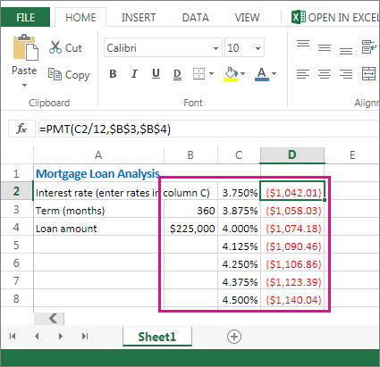
In the following illustration, cell C2 contains the payment formula, =PMT(B3/12,B4,-B5), which uses two input cells, B3 and B4.
Data table calculations
Whenever a worksheet recalculates, any data tables will also recalculate—even if there has been no change to the data. To speed up calculation of a worksheet that contains a data table, you can change the Calculation options to automatically recalculate the worksheet but not the data tables. To learn more, see the section Speed up calculation in a worksheet that contains data tables.
A one-variable data table contain its input values either in a single column (column-oriented), or across a row (row-oriented). Any formula in a one-variable data table must refer to only one input cell.
Follow these steps:
-
Type the list of values that you want to substitute in the input cell—either down one column or across one row. Leave a few empty rows and columns on either side of the values.
-
Do one of the following:
-
If the data table is column-oriented (your variable values are in a column), type the formula in the cell one row above and one cell to the right of the column of values. This one-variable data table is column-oriented, and the formula is contained in cell D2.

If you want to examine the effects of various values on other formulas, enter the additional formulas in cells to the right of the first formula.
-
If the data table is row-oriented (your variable values are in a row), type the formula in the cell one column to the left of the first value and one cell below the row of values.
If you want to examine the effects of various values on other formulas, enter the additional formulas in cells below the first formula.
-
-
Select the range of cells that contains the formulas and values that you want to substitute. In the figure above, this range is C2:D5.
-
On the Data tab, click What-If Analysis > Data Table (in the Data Tools group or Forecast group of Excel 2016).
-
Do one of the following:
-
If the data table is column-oriented, enter the cell reference for the input cell in the Column input cell field. In the figure above, the input cell is B3.
-
If the data table is row-oriented, enter the cell reference for the input cell in the Row input cell field.
Note: After you create your data table, you might want to change the format of the result cells. In the figure, the result cells are formatted as currency.
-
Formulas that are used in a one-variable data table must refer to the same input cell.
Follow these steps
-
Do either of these:
-
If the data table is column-oriented, enter the new formula in a blank cell to the right of an existing formula in the top row of the data table.
-
If the data table is row-oriented, enter the new formula in a empty cell below an existing formula in the first column of the data table.
-
-
Select the range of cells that contains the data table and the new formula.
-
On the Data tab, click What-If Analysis > Data Table (in the Data Tools group or Forecast group of Excel 2016).
-
Do either of the following:
-
If the data table is column-oriented, enter the cell reference for the input cell in the Column input cell box.
-
If the data table is row-oriented, enter the cell reference for the input cell in the Row input cell box.
-
A two-variable data table uses a formula that contains two lists of input values. The formula must refer to two different input cells.
Follow these steps:
-
In a cell on the worksheet, enter the formula that refers to the two input cells.
In the following example—in which the formula starting values are entered in cells B3, B4, and B5, you type the formula =PMT(B3/12,B4,-B5) in cell C2.
-
Type one list of input values in the same column, below the formula.
In this case, type the different interest rates in cells C3, C4, and C5.
-
Enter the second list in the same row as the formula—to its right.
Type the loan terms (in months) in cells D2 and E2.
-
Select the range of cells that contains the formula (C2), both the row and column of values (C3:C5 and D2:E2), and the cells in which you want the calculated values (D3:E5).
In this case, select the range C2:E5.
-
On the Data tab, in the Data Tools group or Forecast group (in Excel 2016), click What-If Analysis > Data Table (in the Data Tools group or Forecast group of Excel 2016).
-
In the Row input cell field, enter the reference to the input cell for the input values in the row.
Type cell B4 in the Row input cell box. -
In the Column input cell field, enter the reference to the input cell for the input values in the column.
Type B3 in the Column input cell box. -
Click OK.
Example of a two-variable data table
A two-variable data table can show how different combinations of interest rates and loan terms will affect a monthly mortgage payment. In the figure here, cell C2 contains the payment formula, =PMT(B3/12,B4,-B5), which uses two input cells, B3 and B4.
When you set this calculation option, no data-table calculations occur when a recalculation is done on the entire workbook. To manually recalculate your data table, select its formulas and then press F9.
Follow these steps to improve calculation performance:
-
Click File > Options > Formulas.
-
In the Calculation options section, under Calculate, click Automatic except for data tables.
Tip: Optionally, on the Formulas tab, click the arrow on Calculation Options, then click Automatic Except Data Tables (in the Calculation group).
You can use a few other Excel tools to perform what-if analysis if you have specific goals or larger sets of variable data.
Goal Seek
If you know the result to expect from a formula, but don’t know precisely what input value the formula needs to get that result, use the Goal-Seek feature. See the article Use Goal Seek to find the result you want by adjusting an input value.
Excel Solver
You can use the Excel Solver add-in to find the optimal value for a set of input variables. Solver works with a group of cells (called decision variables, or simply variable cells) that are used in computing the formulas in the objective and constraint cells. Solver adjusts the values in the decision variable cells to satisfy the limits on constraint cells and produce the result you want for the objective cell. Learn more in this article: Define and solve a problem by using Solver.
By plugging different numbers into a cell, you can quickly come up with different answers to a problem. A great example is using the PMT function with different interest rates and loan periods (in months) to figure out how much of a loan you can afford for a home or a car. You enter your numbers into a range of cells called a data table.
Here, the data table is the range of cells B2:D8. You can change the value in B4, the loan amount, and the monthly payments in column D automatically update. Using a 3.75% interest rate, D2 returns a monthly payment of $1,042.01 using this formula: =PMT(C2/12,$B$3,$B$4).
You can use one or two variables, depending on the number of variables and formulas you want to test.
Use a one-variable test to see how different values of one variable in a formula will change the results. For example, you can change the interest rate for a monthly mortgage payment by using the PMT function. You enter the variable values (the interest rates) in one column or row, and the outcomes are displayed in a nearby column or row.
In this live workbook, cell D2 contains the payment formula =PMT(C2/12,$B$3,$B$4). Cell B3 is the variable cell, where you can plug in a different term length (number of monthly payment periods). In cell D2, the PMT function plugs in the interest rate 3.75%/12, 360 months, and a $225,000 loan, and calculates a $1,042.01 monthly payment.
Use a two-variable test to see how different values of two variables in a formula will change the results. For example, you can test different combinations of interest rates and number of monthly payment periods to calculate a mortgage payment.
In this live workbook, cell C3 contains the payment formula, =PMT($B$3/12,$B$2,B4), which uses two variable cells, B2 and B3. In cell C2, the PMT function plugs in the interest rate 3.875%/12, 360 months, and a $225,000 loan, and calculates a $1,058.03 monthly payment.
Need more help?
You can always ask an expert in the Excel Tech Community or get support in the Answers community.
I have multiple tables in Excel 2016 data model. These tables come from data maintained in other excel worksheets and are imported through Excel Query to populate a data model to take advantage of superior data management features that are available (e.g., DAX, date tables, relational joins, etc.)
However, I would like to be able to create «calculated tables» (with DAX expressions) by applying filters, unions, etc. to target and transform the existing data elements. The goal to use the «calculated tables» in the Data Model for pivot tables, etc. Is this possible within Excel 2016? If not, what complementary tools (apart from SQL) are necessary? TIA.
asked Dec 16, 2017 at 17:25
![]()
JMKõJMKõ
511 silver badge7 bronze badges
2
As of now (August 2019), Excel does not support generation of calculated tables using DAX. I personally believe Microsoft should consider this, given that DAX is efficient in data aggregation and analysis.
Get and Transform
Until having the feature implemented by Microsoft, there is a good alternative within Excel (versions from 2010 onward) by utilizing Get and Transform (called also PowerQuery in older versions).
Using this tool, you will be able to load the same data set (table or other data source) and transform it as a separate table into the data model.
Advantages:
- It is powerful in terms of source data conversion, which extends beyond simple filtering and can deal with importing raw data extracts.
I personally used this approach, and has saved me tremendous time.
Disadvantage:
- Get and Transform is a slower and indirect solution compared to DAX.
- You need to refresh the query sources, whenever there is change of the source data.
Where is it located
- In Excel 2016, to Get and Transform Tool is available Data/New Query.
Please let me know if you need any further explanation to my answer.
answered Aug 22, 2019 at 11:43
![]()
Yes, it is possible to add DAX tables to data model in Excel.

- Use Existing Connection to get whatever table to Excel sheet.

Right click on a table and select Edit DAX. Then shape your DAX code after EVALUATE command.

Add this new DAX shaped table from Excel sheet to your data model.
answered Jan 12, 2022 at 13:17
![]()
Przemyslaw ReminPrzemyslaw Remin
6,09624 gold badges108 silver badges186 bronze badges
0
I don’t think so.
Here (Though i note the article is old):
Unfortunately, calculated tables are not available in Excel 2016. If
you need a similar solution with Excel 2016, you can rely on linked
back tables (i.e. queries over the data model materialized in Excel
tables and then loaded back in the model). The only limitation is that
the size of linked back tables cannot exceed the physical limit of 1M
rows of Excel, whereas DAX calculated tables have no limit in size and
can work in many more scenarios, resulting in a very elegant and neat
model.
I think it is for Power BI particularly using the «New Table» feature and SSAS tabular using new calculated table:
Uses for the New Table Feature in Power BI
This is only available in Power BI Desktop and not in any of the Excel
versions or SSAS Tabular. This feature is essentially a “Calculated
Table” function. You can pass any valid DAX measure that returns a
table of values, and the table will be materialised and loaded into
the data model.
And with SSAS calculated table.
How to create a calculated table
First, verify the tabular model has a compatibility level of 1200 or
higher. You can check the Compatibility Level property on the model in
SSDT.Switch to the Data View. You can’t create a calculated table in
Diagram View.Select Table > New calculated table.
Type or paste a DAX expression (see below for some ideas).
Name the table.
Create relationships to other tables in the model. See Create a
Relationship Between Two Tables (SSAS Tabular) if you need help with
this step.Reference the table in calculations or expressions in your model or
use Analyze in Excel for ad hoc data exploration.
answered Dec 17, 2017 at 13:49
![]()
QHarrQHarr
82.9k11 gold badges55 silver badges99 bronze badges
5
How to Calculate in Excel (Table of Contents)
- Introduction to Calculations in Excel
- Examples of Calculations in Excel
Introduction to Calculations in Excel
The following article provides an outline for Calculations in Excel. MS Excel is the most preferred option for calculation; most investment bankers and financial analysts use it to do data crunching, prepare presentations, or model data.
There are two ways to perform the Excel calculation: Formula and the second is Function. Where formula is the normal arithmetic operation like summation, multiplication, subtraction, etc. Function is the inbuilt formula like SUM (), COUNT (), COUNTA (), COUNTIF (), SQRT () etc.
Operator Precedence: It will use default order to calculate; if there is some operation in parentheses, then it will calculate that part first, then multiplication or division after that addition or subtraction. It is the same as the BODMAS rule.
Examples of Calculations in Excel
Here are some examples of How to Use Excel to Calculate Basic calculations.
You can download this Calculations Excel Template here – Calculations Excel Template
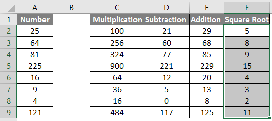
Example #1 – Basic Calculations like Multiplication, Summation, Subtraction, and Square Root
Here we are going to learn how to do basic calculations like multiplication, summation, subtraction, and square root in Excel.
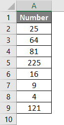
Let’s assume a user wants to perform calculations like multiplication, summation, subtraction by 4 and find out the square root of all numbers in Excel.
Let’s see how we can do this with the help of calculations.
Step 1: Open an Excel sheet. Go to sheet 1 and insert the data as shown below.
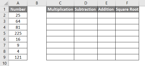
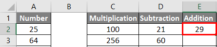
Step 2: Now create headers for Multiplication, Summation, Subtraction, and Square Root in row one.
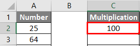
Step 3: Now calculate the multiplication by 4. Use the equal sign to calculate. Write in cell C2 and use asterisk symbol (*) to multiply “=A2*4“

Step 4: Now press on the Enter key; multiplication will be calculated.
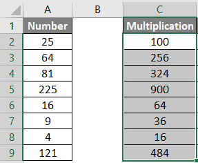
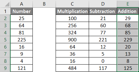
Step 5: Drag the same formula to the C9 cell to apply to the remaining cells.
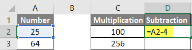
Step 6: Now calculate subtraction by 4. Use an equal sign to calculate. Write in cell D2 “=A2-4“
Step 7: Now click on the Enter key, the subtraction will be calculated.
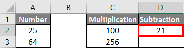
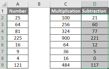
Step 8: Drag the same formula till cell D9 to apply to the remaining cells.
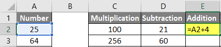
Step 9: Now calculate the addition by 4, use an equal sign to calculate. Write in E2 Cell “=A2+4“
Step 10: Now press on the Enter key, the addition will be calculated.
Step 11: Drag the same formula to the E9 cell to apply to the remaining cells.
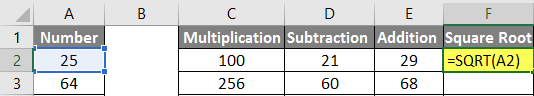
Step 12: Now calculate the square root>> use equal sign to calculate >> Write in F2 Cell >> “=SQRT (A2“
Step 13: Now, press on the Enter key >> square root will be calculated.
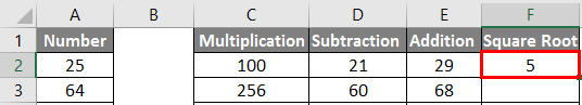
Step 14: Drag the same formula till the F9 cell to apply the remaining cell.
Summary of Example 1: As the user wants to perform calculations like multiplication, summation, subtraction by 4 and find out the square root of all numbers in MS Excel.
Example #2 – Basic Calculations like Summation, Average, and Counting
Here we are going to learn how to use Excel to calculate basic calculations like summation, average, and counting.
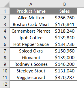
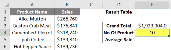
Let’s assume a user wants to find out total sales, average sales, and the total number of products available in his stock for sale.
Let’s see how we can do this with the help of calculations.
Step 1: Open an Excel sheet. Go to Sheet1 and insert the data as shown below.
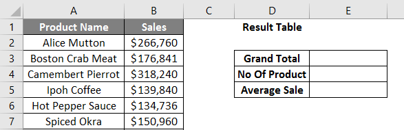
Step 2: Now create headers for Result table, Grand Total, Number of Product and an Average Sale of his product in column D.
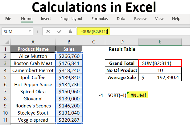
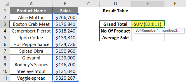
Step 3: Now calculate grand total sales. Use the SUM function to calculate the grand total. Write in cell E3. “=SUM (“
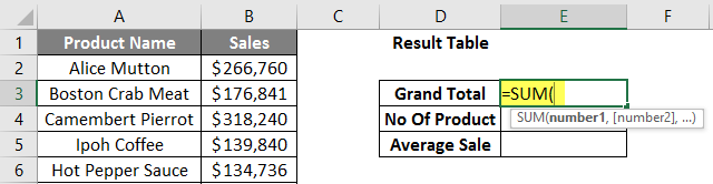
Step 4: Now, it will ask for the numbers, so give the data range, which is available in column B. Write in cell E3. “=SUM (B2:B11) “
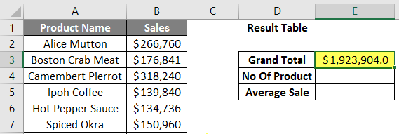
Step 5: Now press on the Enter key. Grand total sales will be calculated.
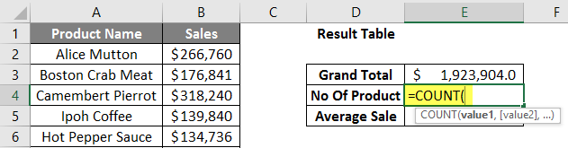
Step 6: Now calculate the total number of products in the stock, use the COUNT function to calculate the grand total. Write in cell E4 “=COUNT (“
Step 7: Now, it will ask for the values, so give the data range, which is available in column B. Write in cell E4. “=COUNT (B2:B11) “
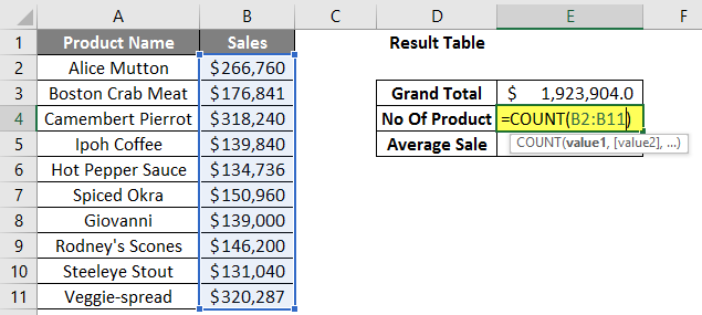
Step 8: Now press on the Enter key. The total number of products will be calculated.
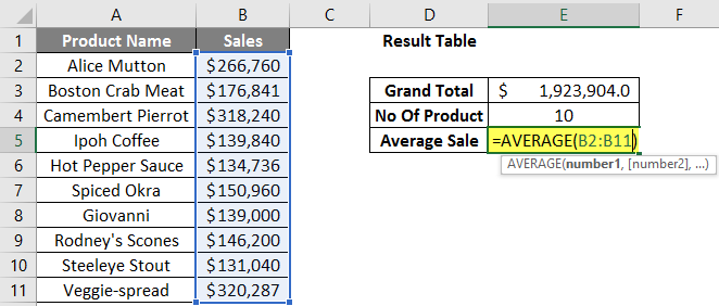
Step 9: Now calculate the average sale of products in the stock, use the AVERAGE function to calculate the average sale. Write in cell E5. “=AVERAGE (“
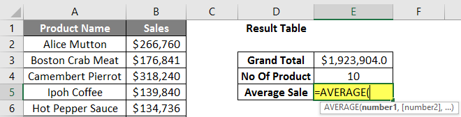
Step 10: Now, it will ask for the numbers, so give the data range which is available in column B. Write in cell E5. “=AVERAGE (B2:B11) “
Step 11: Now click on the Enter key. The average sale of products will be calculated.
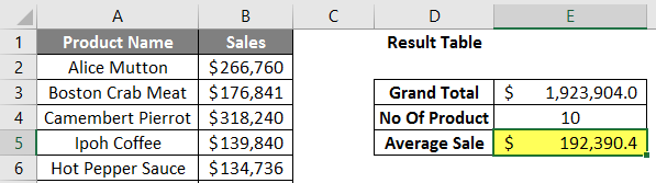
Summary of Example 2: As the user wants to find out total sales, average sales, and the total number of products available in his stock for sale.
Things to Remember about Calculations in Excel
- During calculations, if there are some operations in parentheses, then it will calculate that part first, then multiplication or division after that addition or subtraction.
- It is the same as the BODMAS rule: Parentheses, Exponents, Multiplication and Division, Addition and Subtraction.
- When a user uses an equal sign (=) in any cell, it means that the user is going to put some formula, not a value.
- A small difference from the normal mathematics symbol like multiplication uses asterisk symbol (*) and for division uses forward-slash (/).
- There is no need to write the same formula for each cell; once it is written, then just copy-paste to other cells, it will calculate automatically.
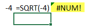
- A user can use the SQRT function to calculate the square root of any value; it has only one parameter. But a user cannot calculate square root for a negative number; it will throw an error #NUM!
- If a negative value occurs as output, use the ABS formula to determine the absolute value, which is an in-built function in MS Excel.
- A user can use the COUNTA in-built function if there is confusion in the data type because COUNT supports only numeric values.
Recommended Articles
This is a guide to Calculations in Excel. Here we discuss how to use excel to calculate along with examples and a downloadable excel template. You may also look at the following articles to learn more –
- Create a Lookup Table in Excel
- Use of COLUMNS Formula in Excel
- CHOOSE Formula in Excel with Examples
- What is Chart Wizard in Excel?
How to Use Excel as a Calculator?
In Excel, by default, there is no calculator button or option available in it. But, we can enable it manually from the “Options” section and then from the “Quick Access Toolbar,” where we can go to the commands not available in the ribbon. There further, we will find the calculator option available. Just click on “Add” and the “OK” to add the calculator to our Excel ribbon.
I have never seen beyond Excel to do the calculations in my career. Most of the calculations are possible with Excel spreadsheets. Not only are the calculations, but they are also flexible enough to reflect the immediate results if there are any modifications to the numbers, which is the power of applying formulas.
By using formulas, we need to worry about all the steps in the calculations because formulas will capture the numbers and show immediate real-time results for us. Excel has hundreds of built-in formulas to work with some of the complex calculations. On top of this, we see the spreadsheet as a mathematics calculator to add, divide, subtract, and multiply.
Table of contents
- How to Use Excel as a Calculator?
- How to Calculate in Excel Sheet?
- Example #1 – Use Formulas in Excel as a Calculator
- Example #2 – Use Cell References
- Example #3 – Cell Reference Formulas are Flexible
- Example #4 – Formula Cell is not Value, It is the only Formula
- Example #5 – Built-In Formulas are Best Suited for Excel
- Recommended Articles
- How to Calculate in Excel Sheet?
This article will show you how to use Excel as a calculator.
How to Calculate in Excel Sheet?
Below are examples of how to use Excel as a calculator.
You can download this Calculation in Excel Template here – Calculation in Excel Template
Example #1 – Use Formulas in Excel as a Calculator
As told, Excel has many of its built-in formulas, and on top of this, we can use Excel in the form of a calculator. To enter anything in the cell, we type the content in the required cell but apply the formula, and we need to start the equal sign in the cell.
Follow the below steps.
- So, to start any calculation, we need first to enter an equal sign, indicating that we are not just entering. Rather, we are entering the formula.

- Once the equal sign is entered in the cell, we can enter the formula. For example, assume that if we want to calculate the addition of two numbers, 50 and 30, we first need to enter the number we want to add.

- Once the number is entered, we need to go back to the basics of mathematics. Since we are doing the addition, we need to apply the PLUS (+) sign.

- After the addition sign (+), we must enter the second number. Then, we need to add to the first number.

- Now, press the ENTER key to get the result in cell A1.


So, 50 + 30 = 80.
It is the basic use of ExcelIn today’s corporate working and data management process, Microsoft Excel is a powerful tool.» Every employee is required to have this expertise. The primary uses of Excel are as follows: Data Analysis and Interpretation, Data Organizing and Restructuring, Data Filtering, Goal Seek Analysis, Interactive Charts and Graphs.
read more as a calculator. Similarly, we can use cell references to the formulaCell reference in excel is referring the other cells to a cell to use its values or properties. For instance, if we have data in cell A2 and want to use that in cell A1, use =A2 in cell A1, and this will copy the A2 value in A1.read more.
Example #2 – Use Cell References
For example, look at the below values in cells A1, A2, and A3.

- We must open an equal sign in the A4 cell.

- Then, select cell A1 first.

- After selecting cell A1, we need to put a plus sign and choose the A2 cell.

- Now, put one more plus sign and select A3 cell.
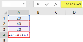
- Press the “ENTER” key to get the result in the A4 cell.
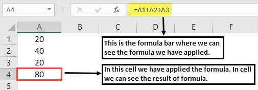
It is the result of using cell references.
Example #3 – Cell Reference Formulas are Flexible
By using cell references, we can make the formula real-time and flexible. We said cell reference formulas are flexible because if we make any changes to the formula input cells (A1, A2, A3), it will reflect the changes in the formula cell (A4).
- We will change the number in cell A2 from 40 to 50.

We have changed the number but have not yet pressed the “ENTER” key. If we hit the “ENTER” key, we can see the result in the A4 cell.
- The moment we press the “ENTER” key, we see the impact on cell A4.
Example #4 – Formula Cell is not Value, It is the only Formula
We need to know when we use a cell reference for formulas because formula cells hold the result of the formula, not the value itself.
- Suppose we have a value of 50 in cell C2.

- If we copy and paste it to the next cell, we still get the value of 50 only.

- But, now come back to cell A4.

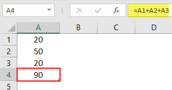
- Here we can see 90, but this is not the value but the formula. So we will copy and paste it to the next cell and see what we get.

Oh oh!!! We got zero.
We got zero because cell A4 has the formula =A1 + A2 + A3. When we copy cell A4 and paste it to B4, formula-referenced cells are changed from A1 + A2 + A3 to B1 + B2 + B3.
We got zero since there are no values in the cells B1, B2, and B3. So now, we will put 60 in any of the cells in B1, B2, and B3 and see the result.

- Look here the moment we have entered 60; we got the result as 60 because cell B4 already has the cell reference of the above three cells (B1, B2, and B3).

Example #5 – Built-In Formulas are Best Suited for Excel
We have seen how to use cell references for the formulas in the above examples. But those are best suited only for the small number of data sets, for a maximum of 5 to 10 cells.
Now, look at the below data.

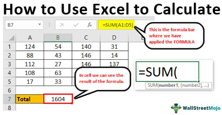
We have numbers from A1 to D5, and in the B7 cell, we need the total of these numbers. In these large data sets, we cannot give individual cell references, which takes a lot of time for us. That is where Excel’s built-in formulas come into the example.
- We should first open the SUM functionThe SUM function in excel adds the numerical values in a range of cells. Being categorized under the Math and Trigonometry function, it is entered by typing “=SUM” followed by the values to be summed. The values supplied to the function can be numbers, cell references or ranges.read more in cell B7.

- Now, hold the left-click of the mouse and select the range of cells from A1 to D5.

- After that, close the bracket and press the “Enter” key.

So, like this, we can use built-in formulas to work with large data sets.
This way, we can calculate in the Excel sheet.
Recommended Articles
This article is a guide to Excel as a Calculator. Here, we discuss how to do a calculation in an Excel sheet with examples and downloadable Excel templates. You may also look at these useful functions in Excel: –
- Calculate Percentage in Excel Formula
- Multiply in Excel Formula
- How to Divide using Excel Formulas?
- Excel Subtraction Formula
Often, once you create a Pivot table, there is a need you to expand your analysis and include more data/calculations as a part of it.
If you need a new data point that can be obtained by using existing data points in the Pivot Table, you don’t need to go back and add it in the source data. Instead, you can use a Pivot Table Calculated Field to do this.
Download the dataset and follow along.
What is a Pivot Table Calculated Field?
Let’s start with a basic example of a Pivot Table.
Suppose you have a dataset of retailers and you create a Pivot Table as shown below:
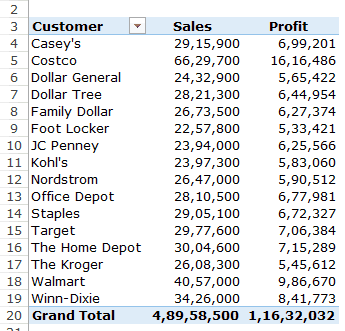
The above Pivot Table summarizes the sales and profit values for the retailers.
Now, what if you also want to know what was the profit margin of these retailers (where the profit margin is ‘Profit’ divided by ‘Sales’).
There are a couple of ways to do this:
- Go back to the original data set and add this new data point. So you can insert a new column in the source data and calculate the profit margin in it. Once you do this, you need to update the source data of the Pivot Table to get this new column as a part of it.
- While this method is a possibility, you would need to manually go back to the data set and make the calculations. For example, you may need to add another column to calculate the average sale per unit (Sales/Quantity). Again you will have to add this column to your source data and then update the pivot table.
- This method also bloats your Pivot Table as you’re adding new data to it.
- Add calculations outside the Pivot Table. This can be an option if your Pivot Table structure is unlikely to change. But if you change the Pivot table, the calculation may not update accordingly and might give you the wrong results or errors. As shown below, I calculated the Profit Margin when there were retailers in the row. But when I changed it from customers to regions, the formula gave an error.

- Using a Pivot Table Calculated Field. This is the most efficient way to use existing Pivot Table data and calculate the desired metric. Consider Calculated Field as a virtual column that you have added using the existing columns from the Pivot Table. There are a lot of benefits of using a Pivot Table Calculated Field (as we will see in a minute):
- It doesn’t require you to handle formulas or update source data.
- It’s scalable as it will automatically account for any new data that you may add to your Pivot Table. Once you add a Calculate Field, you can use it like any other field in your Pivot Table.
- It easy to update and manage. For example, if the metrics change or you need to change the calculation, you can easily do that from the Pivot Table itself.

Adding a Calculated Field to the Pivot Table
Let’s see how to add a Pivot Table Calculated Field in an existing Pivot Table.
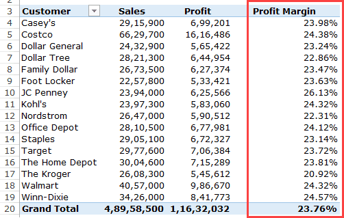
Suppose you have a Pivot Table as shown below and you want to calculate the profit margin for each retailer:
Here are the steps to add a Pivot Table Calculated Field:
As soon as you add the Calculated Field, it will appear as one of the fields in PivotTable Fields list.

Now you can use this calculated field as any other Pivot Table field (note that you can not use Pivot Table Calculated Field as a report filter or slicer).
As I mentioned before, the benefit of using a Pivot Table Calculated Field is that you can change the structure of the Pivot Table and it will automatically adjust.
For example, if I drag and drop region in the rows area, you will get the result as shown below, where Profit Margin value is reported for retailers as well as the region.
 In the above example, I have used a simple formula (=Profit/Sales) to insert a calculated field. However, you can also use some advanced formulas.
Before I show you an example of using an advanced formula to create a Pivot Table Calculate Field, here are some things you must know:
- You CAN NOT use references or named ranges while creating a Pivot Table Calculated Field. That would rule out a lot of formulas such as VLOOKUP, INDEX, OFFSET, and so on. However, you can use formulas that can work without references (such SUM, IF, COUNT, and so on..).
- You can use a constant in the formula. For example, if you want to know the forecasted sales where it is forecasted to grow by 10%, you can use the formula =Sales*1.1 (where 1.1 is constant).
- The order of precedence is followed in the formula that makes the calculated field. As a best practice, use parenthesis to make sure you don’t have to remember the order of precedence.
Now, let’s see an example of using an advanced formula to create a Calculated Field.
Suppose you have the dataset as shown below and you need to show the forecasted sales value in the Pivot Table.
For forecasted value, you need to use a 5% sales increase for large retailers (sales above 3 million) and a 10% sales increase for small and medium retailers (sales below 3 million).
Note: The sales numbers here are fake and have been used to illustrate the examples in this tutorial.
Here is how to do this:
This adds a new column to the pivot table with the sales forecast value.
Click here to Download the dataset.
An Issue With Pivot Table Calculated Fields
Calculated Field is an amazing feature that really enhances the value of your Pivot Table with field calculations, while still keep everything scalable and manageable.
There is, however, an issue with Pivot Table Calculated Fields that you must know before using it.
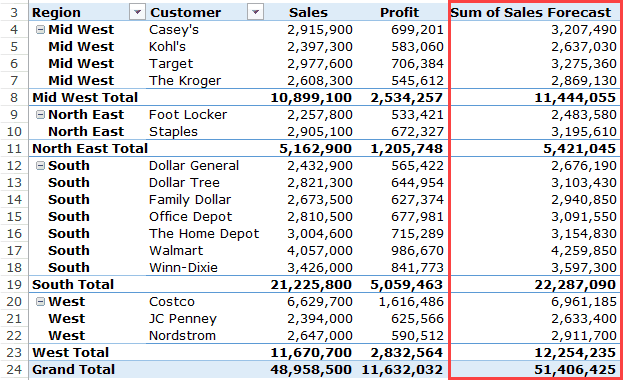
Suppose, I have a Pivot Table as shown below where I used the calculated field to get the forecast sales numbers.
Note that the subtotal and grand totals are not correct.
While these should add the individual sales forecast value for each retailer, in reality, it follows the same calculated field formula that we created.
So for South Total, while the value should be 22,824,000, the South Total wrongly reports it as 22,287,000. This happens as it uses the formula 21,225,800*1.05 to get the value.

Unfortunately, there is no way you can correct this.
The best way to handle this would be to remove subtotals and Grand Totals from your Pivot Table.
You can also go through some innovative workarounds Debra has shown to handle this issue.
How to Modify or Delete a Pivot Table Calculated Field?
Once you have created a Pivot Table Calculated Field, you can modify the formula or delete it using the following steps:
How to Get a List of All the Calculated Field Formulas?
If you create a lot of Pivot Table Calculated field, don’t worry about keeping track of the formula used in each one of it.
Excel allows you to quickly create a list of all the formulas used in creating Calculated Fields.
Here are the steps to quickly get the list of All Calculated Fields formulas:
- Select any cell in the Pivot Table.
- Go to Pivot Table Tools –> Analyze –> Fields, Items, & Sets –> List Formulas.

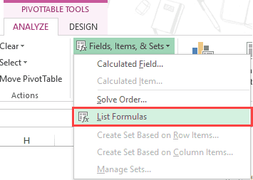
As soon as you click on List Formulas, Excel would automatically insert a new worksheet that will have the details of all the calculated fields/items that you have used in the Pivot Table.
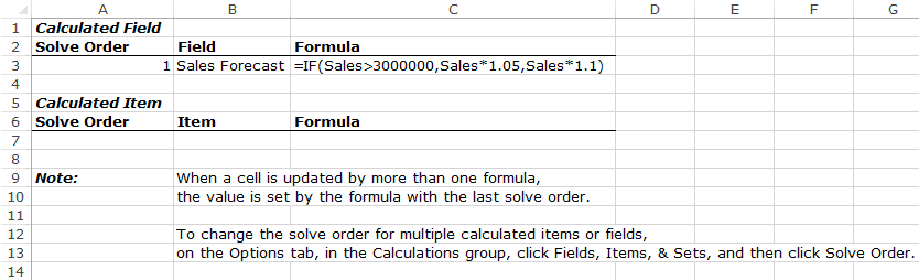
This can be a really useful tool if you have to send your work to the client or share it with your team.
You May Also Find the following Pivot Table Tutorials Useful:
- Preparing Source Data For Pivot Table.
- Using Slicers in Excel Pivot Table: A Beginner’s Guide.
- How to Group Dates in Pivot Tables in Excel.
- How to Group Numbers in Pivot Table in Excel.
- How to Filter Data in a Pivot Table in Excel.
- How to Replace Blank Cells with Zeros in Excel Pivot Tables.
- How to Apply Conditional Formatting in a Pivot Table in Excel.
- Pivot Cache in Excel – What Is It and How to Best Use It?
- How to Delete a Pivot Table in Excel
- How to Show Pivot Table Fields List? (Get Pivot Table Menu Back)