
Use Excel as your calculator
Instead of using a calculator, use Microsoft Excel to do the math!
You can enter simple formulas to add, divide, multiply, and subtract two or more numeric values. Or use the AutoSum feature to quickly total a series of values without entering them manually in a formula. After you create a formula, you can copy it into adjacent cells — no need to create the same formula over and over again.
Subtract in Excel

Multiply in Excel
Divide in Excel
Learn more about simple formulas
All formula entries begin with an equal sign (=). For simple formulas, simply type the equal sign followed by the numeric values that you want to calculate and the math operators that you want to use — the plus sign (+) to add, the minus sign (—) to subtract, the asterisk (*) to multiply, and the forward slash (/) to divide. Then, press ENTER, and Excel instantly calculates and displays the result of the formula.
For example, when you type =12.99+16.99 in cell C5 and press ENTER, Excel calculates the result and displays 29.98 in that cell.
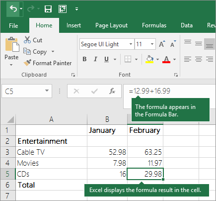
The formula that you enter in a cell remains visible in the formula bar, and you can see it whenever that cell is selected.
Important: Although there is a SUM function, there is no SUBTRACT function. Instead, use the minus (-) operator in a formula; for example, =8-3+2-4+12. Or, you can use a minus sign to convert a number to its negative value in the SUM function; for example, the formula =SUM(12,5,-3,8,-4) uses the SUM function to add 12, 5, subtract 3, add 8, and subtract 4, in that order.
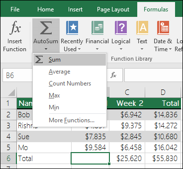
Use AutoSum
The easiest way to add a SUM formula to your worksheet is to use AutoSum. Select an empty cell directly above or below the range that you want to sum, and on the Home or Formula tabs of the ribbon, click AutoSum > Sum. AutoSum will automatically sense the range to be summed and build the formula for you. This also works horizontally if you select a cell to the left or right of the range that you need to sum.
Note: AutoSum does not work on non-contiguous ranges.
AutoSum vertically
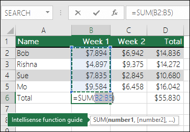
In the figure above, the AutoSum feature is seen to automatically detect cells B2:B5 as the range to sum. All you need to do is press ENTER to confirm it. If you need to add/exclude more cells, you can hold the Shift Key + the arrow key of your choice until your selection matches what you want. Then press Enter to complete the task.
Intellisense function guide: the SUM(number1,[number2], …) floating tag beneath the function is its Intellisense guide. If you click the SUM or function name, it will change o a blue hyperlink to the Help topic for that function. If you click the individual function elements, their representative pieces in the formula will be highlighted. In this case, only B2:B5 would be highlighted, since there is only one number reference in this formula. The Intellisense tag will appear for any function.
AutoSum horizontally

Learn more in the article on the SUM function.
Avoid rewriting the same formula
After you create a formula, you can copy it to other cells — no need to rewrite the same formula. You can either copy the formula, or use the fill handle  to copy the formula to adjacent cells.
For example, when you copy the formula in cell B6 to C6, the formula in that cell automatically changes to update to cell references in column C.
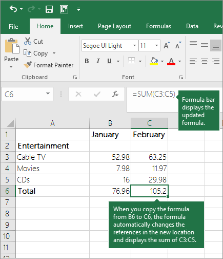
When you copy the formula, ensure that the cell references are correct. Cell references may change if they have relative references. For more information, see Copy and paste a formula to another cell or worksheet.
What can I use in a formula to mimic calculator keys?
|
Calculator key |
Excel method |
Description, example |
Result |
|
+ (Plus key) |
+ (plus) |
Use in a formula to add numbers. Example: =4+6+2 |
12 |
|
— (Minus key) |
— (minus) |
Use in a formula to subtract numbers or to signify a negative number. Example: =18-12 Example: =24*-5 (24 times negative 5) |
-120 |
|
x (Multiply key) |
* (asterisk; also called «star») |
Use in a formula to multiply numbers. Example: =8*3 |
24 |
|
÷ (Divide key) |
/ (forward slash) |
Use in a formula to divide one number by another. Example: =45/5 |
9 |
|
% (Percent key) |
% (percent) |
Use in a formula with * to multiply by a percent. Example: =15%*20 |
3 |
|
√ (square root) |
SQRT (function) |
Use the SQRT function in a formula to find the square root of a number. Example: =SQRT(64) |
8 |
|
1/x (reciprocal) |
=1/n |
Use =1/n in a formula, where n is the number you want to divide 1 by. Example: =1/8 |
0.125 |
Need more help?
You can always ask an expert in the Excel Tech Community or get support in the Answers community.
Need more help?
Want more options?
Explore subscription benefits, browse training courses, learn how to secure your device, and more.
Communities help you ask and answer questions, give feedback, and hear from experts with rich knowledge.
Return to Excel Formulas List
Download Example Workbook
Download the example workbook
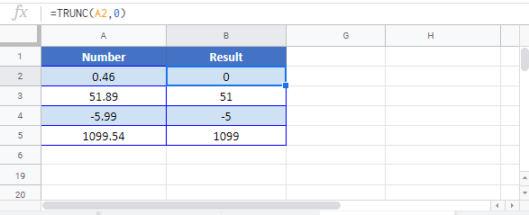
This tutorial will demonstrate how to calculate the integer portion of a number in Excel and Google Sheets.
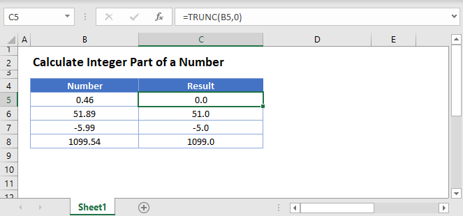
Integer Portion of Number
To calculate the integer portion of a number, use the TRUNC Function to “truncate” off the decimal.
=TRUNC(B3,0)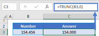
The TRUNC Function simply cuts off the decimal, it does not round.
INT and ROUND Functions
You might be wondering about the INT or ROUND Functions.
The INT Function will work exactly the same as TRUNC for positive numbers, but for negative numbers INT rounds numbers down away from zero.
=INT(B3)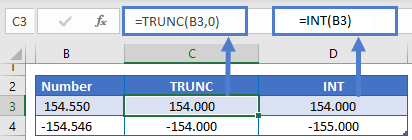
The ROUND Function rounds number, which can give different answers than the other functions.
=ROUND(B3,0)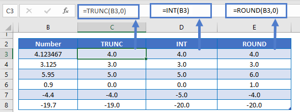
Calculate Integer Part of a Number in Google Sheets
All of the above examples work exactly the same in Google Sheets as in Excel.
In this example, the goal is to calculate various percentages of the number in cell B5. This is a straightforward calculation in Excel. The main task is to correctly enter the numbers in column D as percentages. Once that is done, you can multiply the percentage by the number.
The first step is to format the cells in the range D5:D12 with the percentage number format. You can use the keyboard shortcut Control + Shift + %. Once the cells are correctly formatted, you can enter the numbers without the % operator. Excel will automatically add the % sign.
Next, enter the formula in cell E5. This formula simply multiplies the amount in B5 by the percentage in D5:
=$B$5*D5
Because the formula will be copied down, the reference to cell B5 must be an absolute reference. This locks the reference and prevents changes as the formula is copied down. Because the reference to cell D5 is relative, it will change at each new row.
The results in column E are the amounts of B5 that correspond with each percentage in column D. If the number in B5 is changed, the results in column E are updated.
Note: the percentages in column D are completely arbitrary and can be changed as desired.
In Excel, we can easily add the digits of a number. Usually, calculations that involve multiple values can be dealt with the help of array formulas, but here, we are going to find the sum of the digits of a number using non-array formulas. As an example, say we have a number 238 in one of the cells of the Excel sheet and we want to find the sum of the digits of this number. It would essentially be 2 + 3 + 8 which equals 13. Let us see how to do that without using an array formula. But before jumping on to the non-array formula method of finding the sum of the digits of a number, let us first see what is an array formula.
Array Formula
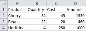
An array formula is nothing but a method that enables one to do multiple calculations at once. It can also do a calculation more than once in a specific cell range. Look at the example below. Say we have to find the product of quantities and cost as shown in the excel sheet below. If we do this using an array formula, then we can get the result much faster.
We can use the multi-cell array formula for multiplying the quantity and cost column.
Multi-cell array formula
Here, we have to use a single formula and we will get results of all the rows. To calculate all the values of the Amount table, we will first select the area where we want to see the end result. Press F2 after selecting the required area so that you come back on to the first cell of the selected area.
Then, write the array formula in the first cell where the cursor is placed. The formula is simply: =B2:B4*C2:C4
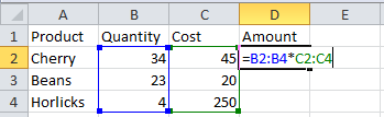
Now, don’t just press enter because then it will print the result in only one cell. These formulas are CSE, meaning they will execute properly only when you click CTRL + SHIFT + ENTER. See the result.
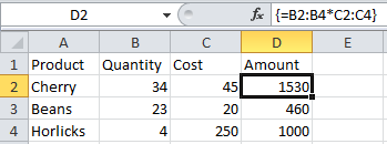
Note that Excel automatically adds curly braces around the formula. This is to indicate that it is an array formula.
Non-array Formula
There are two non-array formulas that we can use to find the sum of the digits of a number. These are:
- Sum and Index Formula
- Sumproduct and Indirect Formula
Let us look at them one by one.
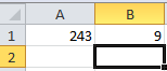
1. Sum and Index formula: Here, we have a number 243 and we have to find the sum of its digits. We will go to the cell in which we want to get the sum and write the following formula:
=SUM(INDEX(1*(MID(A1,ROW(INDIRECT(“1:”&LEN(A1))),1)),,))
This formula uses various functions. Let us understand this formula a bit more:
- The INDEX function will return the value at a given location. In this case, it would be the value of these numbers.
- The MID function will return a sequence of values from the middle of the string. In this case, the string is nothing but the number itself.
- The ROW function will simply return the number for the referenced. Here the row number will be A1.
- The INDIRECT function will return a valid cell reference from this string of numbers.
- The LEN function will return the number of characters of the string. In this case, it would be 3.
Sum and Index formula

Just press Enter and you will get the result.
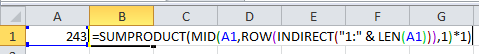
2. Sumproduct and Indirect Formula: Again we have a number 243 and we have to find the sum of its digits. We will go to the cell in which we want to get the sum and write the following formula:
=SUMPRODUCT(MID(A1,ROW(INDIRECT(“1:” & LEN(A1))),1)*1)
There is one more formula under this category that works the same:
=SUMPRODUCT(MID(A1,ROW(OFFSET($A$1,,,LEN(A1))),1)+0)
It is shown here:
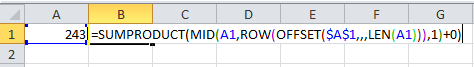
Both these formulae give the same output:
A few more functions are used in this formula. These are:
- The OFFSET function will return a range specifying a certain number of rows and columns to address a cell.
- The SUMPRODUCT function first multiplies a range of cells and then returns the sum of the product.
How to Calculate in Excel (Table of Contents)
- Introduction to Calculations in Excel
- Examples of Calculations in Excel
Introduction to Calculations in Excel
The following article provides an outline for Calculations in Excel. MS Excel is the most preferred option for calculation; most investment bankers and financial analysts use it to do data crunching, prepare presentations, or model data.
There are two ways to perform the Excel calculation: Formula and the second is Function. Where formula is the normal arithmetic operation like summation, multiplication, subtraction, etc. Function is the inbuilt formula like SUM (), COUNT (), COUNTA (), COUNTIF (), SQRT () etc.
Operator Precedence: It will use default order to calculate; if there is some operation in parentheses, then it will calculate that part first, then multiplication or division after that addition or subtraction. It is the same as the BODMAS rule.
Examples of Calculations in Excel
Here are some examples of How to Use Excel to Calculate Basic calculations.
You can download this Calculations Excel Template here – Calculations Excel Template
Example #1 – Basic Calculations like Multiplication, Summation, Subtraction, and Square Root
Here we are going to learn how to do basic calculations like multiplication, summation, subtraction, and square root in Excel.
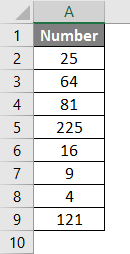
Let’s assume a user wants to perform calculations like multiplication, summation, subtraction by 4 and find out the square root of all numbers in Excel.
Let’s see how we can do this with the help of calculations.
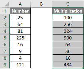
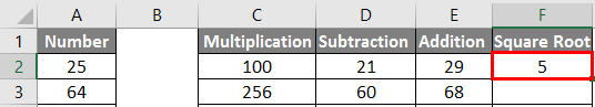
Step 1: Open an Excel sheet. Go to sheet 1 and insert the data as shown below.
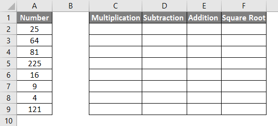
Step 2: Now create headers for Multiplication, Summation, Subtraction, and Square Root in row one.
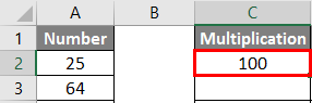
Step 3: Now calculate the multiplication by 4. Use the equal sign to calculate. Write in cell C2 and use asterisk symbol (*) to multiply “=A2*4“

Step 4: Now press on the Enter key; multiplication will be calculated.
Step 5: Drag the same formula to the C9 cell to apply to the remaining cells.
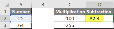
Step 6: Now calculate subtraction by 4. Use an equal sign to calculate. Write in cell D2 “=A2-4“
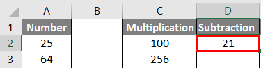
Step 7: Now click on the Enter key, the subtraction will be calculated.
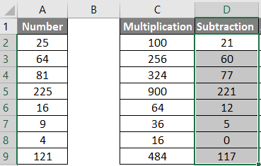
Step 8: Drag the same formula till cell D9 to apply to the remaining cells.
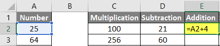
Step 9: Now calculate the addition by 4, use an equal sign to calculate. Write in E2 Cell “=A2+4“
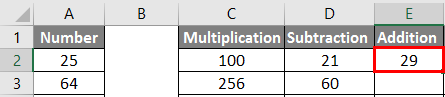
Step 10: Now press on the Enter key, the addition will be calculated.
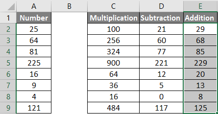
Step 11: Drag the same formula to the E9 cell to apply to the remaining cells.
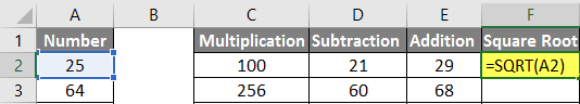
Step 12: Now calculate the square root>> use equal sign to calculate >> Write in F2 Cell >> “=SQRT (A2“
Step 13: Now, press on the Enter key >> square root will be calculated.
Step 14: Drag the same formula till the F9 cell to apply the remaining cell.
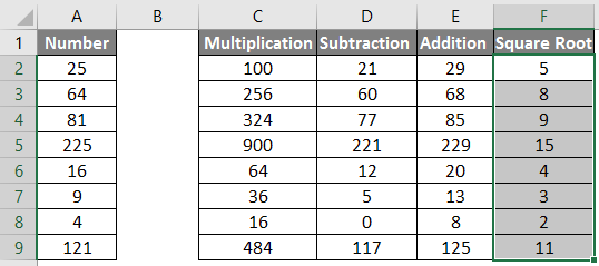
Summary of Example 1: As the user wants to perform calculations like multiplication, summation, subtraction by 4 and find out the square root of all numbers in MS Excel.
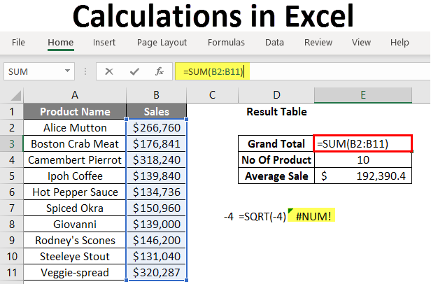
Example #2 – Basic Calculations like Summation, Average, and Counting
Here we are going to learn how to use Excel to calculate basic calculations like summation, average, and counting.
Let’s assume a user wants to find out total sales, average sales, and the total number of products available in his stock for sale.
Let’s see how we can do this with the help of calculations.
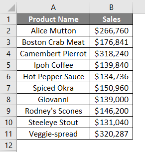
Step 1: Open an Excel sheet. Go to Sheet1 and insert the data as shown below.
Step 2: Now create headers for Result table, Grand Total, Number of Product and an Average Sale of his product in column D.
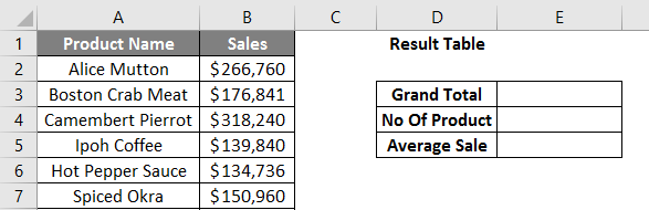
Step 3: Now calculate grand total sales. Use the SUM function to calculate the grand total. Write in cell E3. “=SUM (“
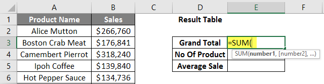
Step 4: Now, it will ask for the numbers, so give the data range, which is available in column B. Write in cell E3. “=SUM (B2:B11) “
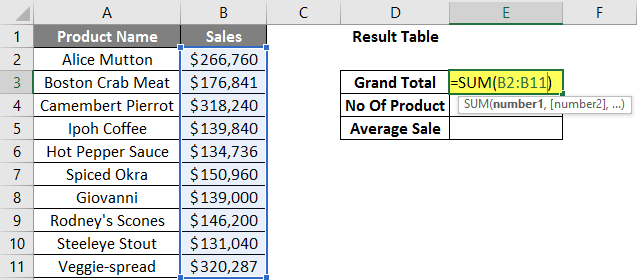
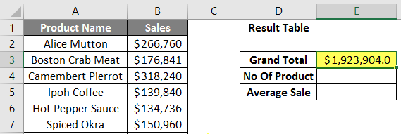
Step 5: Now press on the Enter key. Grand total sales will be calculated.
Step 6: Now calculate the total number of products in the stock, use the COUNT function to calculate the grand total. Write in cell E4 “=COUNT (“
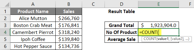
Step 7: Now, it will ask for the values, so give the data range, which is available in column B. Write in cell E4. “=COUNT (B2:B11) “
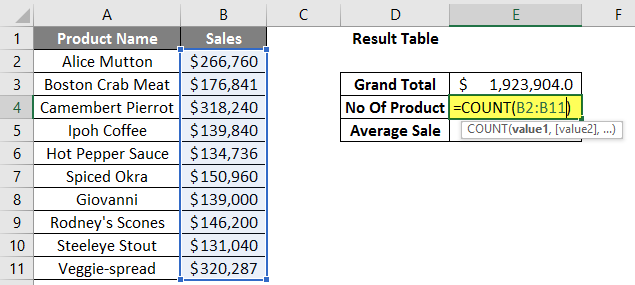
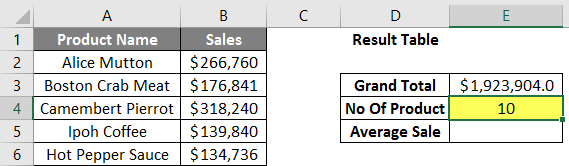
Step 8: Now press on the Enter key. The total number of products will be calculated.
Step 9: Now calculate the average sale of products in the stock, use the AVERAGE function to calculate the average sale. Write in cell E5. “=AVERAGE (“
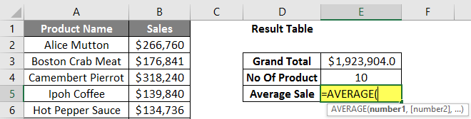
Step 10: Now, it will ask for the numbers, so give the data range which is available in column B. Write in cell E5. “=AVERAGE (B2:B11) “
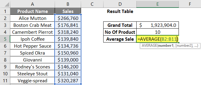
Step 11: Now click on the Enter key. The average sale of products will be calculated.
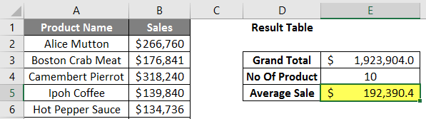
Summary of Example 2: As the user wants to find out total sales, average sales, and the total number of products available in his stock for sale.
Things to Remember about Calculations in Excel
- During calculations, if there are some operations in parentheses, then it will calculate that part first, then multiplication or division after that addition or subtraction.
- It is the same as the BODMAS rule: Parentheses, Exponents, Multiplication and Division, Addition and Subtraction.
- When a user uses an equal sign (=) in any cell, it means that the user is going to put some formula, not a value.
- A small difference from the normal mathematics symbol like multiplication uses asterisk symbol (*) and for division uses forward-slash (/).
- There is no need to write the same formula for each cell; once it is written, then just copy-paste to other cells, it will calculate automatically.
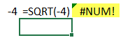
- A user can use the SQRT function to calculate the square root of any value; it has only one parameter. But a user cannot calculate square root for a negative number; it will throw an error #NUM!
- If a negative value occurs as output, use the ABS formula to determine the absolute value, which is an in-built function in MS Excel.
- A user can use the COUNTA in-built function if there is confusion in the data type because COUNT supports only numeric values.
Recommended Articles
This is a guide to Calculations in Excel. Here we discuss how to use excel to calculate along with examples and a downloadable excel template. You may also look at the following articles to learn more –
- Create a Lookup Table in Excel
- Use of COLUMNS Formula in Excel
- CHOOSE Formula in Excel with Examples
- What is Chart Wizard in Excel?