Calculate number of days excel

This article describes the formula syntax and usage of the DAYS function in Microsoft Excel. For information about the DAY function, see DAY function.

Description

Returns the number of days between two dates.

Syntax

DAYS(end_date, start_date)

The DAYS function syntax has the following arguments.

• End_date    Required. Start_date and End_date are the two dates between which you want to know the number of days.

• Start_date   
  Required. Start_date and End_date are the two dates between which you want to know the number of days.

Note: Excel stores dates as sequential serial numbers so that they can be used in calculations. By default, Jan 1, 1900 is serial number 1, and January 1, 2008 is serial number 39448 because it is 39447 days after January 1, 1900.

Remarks

• If both date arguments are numbers, DAYS uses EndDate–StartDate to calculate the number of days in between both dates.

• If either one of the date arguments is text, that argument is treated as DATEVALUE(date_text) and returns an integer date instead of a time component.

• If date arguments are numeric values that fall outside the range of valid dates, DAYS returns the #NUM! error value.

• If date arguments are strings that cannot be parsed as valid dates, DAYS returns the #VALUE! error value.

Example

Copy the example data in the following table, and paste it in cell A1 of a new Excel worksheet. For formulas to show results, select them, press F2, and then press Enter. If you need to, you can adjust the column widths to see all the data.

Data
31-DEC-2021
1-JAN-2021
Formula	Description	Result
=DAYS(«15-MAR-2021″,»1-FEB-2021»)	Finds the number of days between the end date (15-MAR-2021) and start date (1-FEB-2021). When you enter a date directly in the function, you need to enclose it in quotation marks. Result is 42.	42
=DAYS(A2,A3)	Finds the number of days between the end date in A2 and the start date in A3 (364).	364

Top of Page

Summary

The Excel DAYS function returns the number of days between two dates. With a start date in A1 and end date in B1, =DAYS(B1,A1) will return the days between the two dates.

Purpose 

Return value 

A number representing days.

Arguments 

• end_date — The end date.
• start_date — The start date.

Syntax 

=DAYS(end_date, start_date)

Usage notes 

The DAYS function returns the number of days between two dates. Both dates must be valid Excel dates or text values that can be coerced to dates. The DAYS function only works with whole numbers, fractional time values that might be part of a date are ignored. If start and end dates are reversed, DAYS returns a negative number. The DAYS function returns all days between two dates, to calculate working days between dates, see the NETWORKDAYS function.

Examples

With a start date in A1 and end date in A2:

=DAYS(A2,A1)

Will return the same result as:

=A2-A1

Unlike the simple formula above, the DAYS function can also handle dates in text format, as long as the date is recognized by Excel. For example:

=DAYS("7/15/2016","7/1/2016") // returns 14

The DAYS function returns the number of days between two dates. For example:

=DAYS("1-Mar-21","2-Mar-21") // returns 1

To include the end date in the count, add 1 to the result:

=DAYS("1-Mar-21","2-Mar-21")+1 // returns 2

Storing and parsing text values that represent dates should be avoided, because it can introduce errors and parsing problems. Working with native Excel dates (which are numbers) is a better approach. To create a numeric date from scratch in a formula, use the DATE function.

Notes

• The DAYS function only works with whole numbers and ignores time.
• If dates are not recognized, DAYS returns the #VALUE! error.
• If dates are out of range, DAYS returns the #NUM! error.

Author

Dave Bruns

Hi — I’m Dave Bruns, and I run Exceljet with my wife, Lisa. Our goal is to help you work faster in Excel. We create short videos, and clear examples of formulas, functions, pivot tables, conditional formatting, and charts.

Watch Video – Calculate the Number of Workdays Between Two Dates

Excel has some powerful functions to calculate the number of days between two dates in Excel. These are especially useful when you’re creating Gantt charts or timelines for a proposal/project.

In this tutorial, you’ll learn how to calculate the number of days between two dates (in various scenarios):

Calculating the Total Number of Days Between Two Dates in Excel

Excel has multiple ways to calculate the days between two dates.

Using the DAYS Function

Excel DAYS function can be used to calculate the total number of days when you have the start and the end date.

You need to specify the ‘Start Date’ and the ‘End Date’ in the Days function, and it will give you the total number of days between the two specified dates.

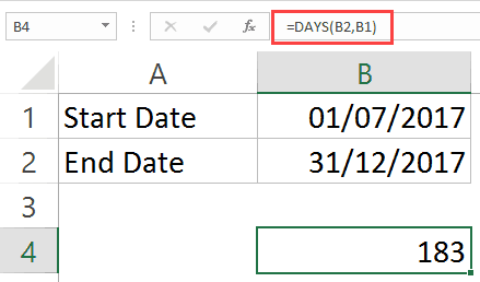
For example, suppose you have the start date is in cell B1 and End Date is in cell B2 (as shown below):

The following formula will give you the total number of days between the two dates:

=DAYS(B2,B1)

Note that you can also manually specify the dates in the Days function by putting it in double-quotes. Just make sure these dates in double-quotes is in an accepted date format in Excel.

Days function gives you the number of days between two dates. This means that if the dates are 1 Dec 2017 and 2 Dec 2017, it will return 1. If you want both the days to be counted, you need to add 1 to the result of Days function. You can read more about the Days function here.

Using the DATEDIF Function

DATEDIF function (derived from Date Difference) also allows you to quickly get the number of days between two dates. But unlike the DAYS function, it can do more than that.

You can also use the DATEDIF function to calculate the number of months or years that have elapsed in the two given dates.

Suppose you have the below dataset and you want to get the number of days between these two dates:

You can use the below DATEDIF formula to do this:

=DATEDIF(B1,B2,"D")

The above DATEDIF formula takes three arguments:

• The start date – B1 in this example
• The end date – B2 in this example
• “D” – the text string that tells the DATEDIF function what needs to be calculated.

Also note that unline the other Excel functions, when you type the DATEDIF function in Excel, it will not show the IntelliSense (the autocomplete option that helps you with the formula arguments).

If you only want to calculate the number of days between two given dates, then it’s better to use the DAYS function. DATEDIF is more suited when you want to calculate the total number of years or months that have passed in between two dates.

For example, the below formula would give you the total number of months between the two dates (in B1 and B2)

=DATEDIF(B1,B2,"M")

Similarly, the below formula will give you the total number of years between the two dates:

=DATEDIF(B1,B2,"Y")

You can read more about the DATEDIF function here. One of the common uses of this function is when you need to calculate age in Excel.

Number of Working Days Between Two Dates in Excel

Excel has two functions that will give you the total number of working days between two dates and will automatically account for weekends and specified holidays.

• Excel NETWORKDAYS function – you should use this when the weekend days are Saturday and Sunday.
• Excel NETWORKDAYS INTERNATIONAL function – use this when the weekend days are not Saturday and Sunday.

Let’s first quickly have a look at NETWORKDAYS Function syntax and arguments.

Excel NETWORKDAYS Function – Syntax & Arguments

=NETWORKDAYS(start_date, end_date, [holidays])

• start_date – a date value that represents the start date.
• end_date – a date value that represents the end date.
• [holidays] – (Optional) It is a range of dates that are excluded from the calculation. For example, these could be national/public holidays. This could be entered as a reference to a range of cells that contains the dates, an array of serial numbers that represent the dates, or a named range.

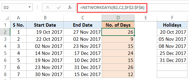
Let’s first look at an example where you want to calculate the number of working days (business days) between two dates with Saturday and Sunday as weekends.

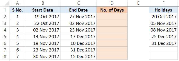
To calculate the number of working days (Column D) – when the start date, end date, and holidays are specified – use the below formula in D3 and copy for all cells:

=NETWORKDAYS(B2,C2,$F$2:$F$6)

This function works great in most cases, except the ones where the weekends are days other than Saturday and Sunday.

For example, in middle-eastern countries, the weekend is Friday and Saturday, or in some jobs, people may have a six-day workweek.

To tackle such cases, Excel has another function – NETWORKDAYS.INTL (introduced in Excel 2010).

Before I take you through the example, let’s quickly learn about the syntax and arguments of Excel NETWORKDAY INTERNATIONAL function

Excel NETWORKDAYS INTERNATIONAL Function – Syntax & Arguments

=NETWORKDAYS.INTL(start_date, end_date, [weekend], [holidays])

• start_date – a date value that represents the start date.
• end_date – a date value that represents the end date.
• [weekend] – (Optional) Here, you can specify the weekend, which could be any two days or any single day. If this is omitted, Saturday and Sunday are taken as the weekend.
• [holidays] – (Optional) It is a range of dates that are excluded from the calculations. For example, these could be national/public holidays. This could be entered as a reference to a range of cells that contains the dates or could be an array of serial numbers that represent the dates.

Now let’s see an example of calculating the number of working days between two dates where the weekend days are Friday and Saturday.

Suppose you have a dataset as shown below:

To calculate the number of working days (Column D) with the weekend as Friday and Saturday, use the following formula:

=NETWORKDAYS.INTL(B2,C2,7,$F$2:$F$6)

The third argument in this formula (the number 7) tells the formula to consider Friday and Saturday as the weekend.

Number of Weekends Between Two Dates in Excel

We can use the NETWORKDAYS function to calculate the number of weekends between two dates.

While the Networkdays function calculates the number of working days, we can also use to get the number of weekend days between two dates.

Suppose we have a dataset as shown below:

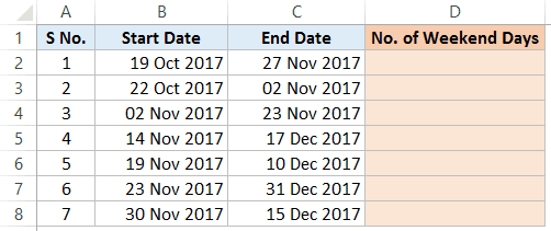
Here is the formula that will give you the total number of weekends days between the two dates:

=DAYS(C2,B2)+1-NETWORKDAYS(B2,C2)

Number of Work Days in a Part-time Job

You can use Excel NETWORKDAYS.INTL function to calculate the number of workdays in a part-time job as well.

Let’s take an example where you are involved in a project where you have to work part-time (Tuesday and Thursday only).

Here is the formula that will get this done:

=NETWORKDAYS.INTL($B$3,$C$3,"1010111",$E$3:$E$7)

Note that instead of choosing the weekend from the drop-down that’s inbuilt in the function, we have used “1010111” (in double quotes).

• 0 indicates a working day
• 1 indicates a non-working day

The first number of this series represents Monday and the last number represents Sunday.

So “0000011“ would mean that Monday to Friday are working days and Saturday and Sunday are non-working (weekend).

With the same logic, “1010111” indicates that only Tuesday and Thursday are working, and rest 5 days are non-working.

In case you have holidays (which you don’t want to get counted in the result), you can specify these holidays as the fourth argument.

Number of Mondays Between Two Dates

To find the number of Mondays between two dates (or any other day), we can use the same logic as used above in calculating part-time jobs.

Suppose you have a dataset as shown below:

Here is the formula that will give you the number of Mondays between the two dates:

=NETWORKDAYS.INTL(B2,C2,"0111111")

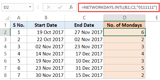
In this formula, ‘0’ means a working day and ‘1’ means a non-working day.

This formula gives us the total number of working days considering that Monday is the only working day of the week.

Similarly, you can also calculate the number of any day between two given dates.

You May Also Like the Following Tutorials:

• Excel Timesheet Calculator Template.
• Convert Date to Text in Excel.
• How to Group Dates in Pivot Tables in Excel.
• How to Automatically Insert Date and Time Stamp in Excel.
• Convert Time to Decimal Number in Excel (Hours, Minutes, Seconds)
• How to SUM values between two dates in Excel
• Get Day Name from Date in Excel
• Check IF a Date is Between Two Given Dates in Excel
• How to Add Week to Date in Excel?

Date yes Add (Subtract) Days to a Date Concatenate Dates Convert Date to Number Convert Date to Text Month Name to Number Create Date Range from Dates Day Number of Year Month Name from Date First Day of Month Add (Subtract) Weeks to a Date If Functions with Dates Max Date Number of Days Between Dates Number of Days in a Month Number of Weeks Between Dates Number of Years Between Dates Split Date & Time into Separate Cells Countdown Remaining Days Insert Dates Random Date Generator Using Dynamic Ranges — Year to Date Values Add (Subtract) Years to a Date Date Formula Examples Extract Day from Date Get Day Name from Date Count Days Left in Month / Year Count Workdays Left in Month / Year Get Last Day of Month Last Business Day of Month / Year Number of Work / Business Days in Month Weekday Abbreviations Auto Populate Dates Number of Months Between Dates Quarter from a Date Years of Service Change Date Format Compare Dates Time yes Add (Subtract) Hours to Time Add (Subtract) Minutes to Time Add (Subtract) Seconds to Time Add Up time (Total Time) Time Differences Change Time Format Convert Minutes to Hours Convert Time to Decimal Convert Time to Hours Convert Time to Minutes Convert Time to Seconds Military Time Round Time to Nearest 15 Minutes Overtime Calculator Number of Hours Between Times Convert Seconds to Minutes, Hours, or Time Count Hours Worked Time Differences Time Format — Show Minutes Seconds Text yes Add Commas to Cells Get First Word from Text Capitalize First Letter Clean & Format Phone #s Remove Extra Trailing / Leading Spaces Add Spaces to Cell Assign Number Value to Text Combine Cells with Comma Combine First and Last Names Convert Text String to Date Convert Text to Number Extract Text From Cell Get Last Word Remove Unwated Characters Extract Text Before or After Character How to Split Text String by Space, Comma, & More Remove Special Characters Remove First Characters from Left Substitute Multiple Values Switch First & Last Names w/ Commas Remove Specific Text from a Cell Extract Text Between Characters (Ex. Parenthesis) Add Leading Zeros to a Number Remove Line Breaks from Text Remove all Numbers from Text Reverse Text Remove Non-Numeric Characters Remove Last Character(s) From Right Separate First and Last Names Separate Text & Numbers Round yes Round Formulas Round Price to Nearest Dollar or Cent Round to Nearest 10, 100, or 1000 Round to Nearest 5 or .5 Round Percentages Round to Significant Figures Count yes Count Blank and Non-blank Cells Count Cells Between Two Numbers Count Cells not Equal to Count if Cells are in Range Count Times Word Appears in Cell Count Words in Cell Count Specific Characters in Column Count Total Number of Characters in Column Count Cells that Equal one of two Results Count Cells that do not Contain Count Cells that Contain Specific Text Count Unique Values in Range Countif — Multiple Criteria Count Total Number of Cells in Range Count Cells with Any Text Count Total Cells in a Table Lookup yes Two Dimensional VLOOKUP VLOOKUP Simple Example Vlookup — Multiple Matches Case Sensitive Lookup Case Sensitive VLOOKUP Sum if — VLOOKUP Case Sensitive Lookup Case Sensitive VLOOKUP Find Duplicates w/ VLOOKUP or MATCH INDEX MATCH MATCH Lookup — Return Cell Address (Not Value) Lookup Last Value in Column or Row Reverse VLOOKUP (Right to Left) Risk Score Bucket with VLOOKUP Sum with a VLOOKUP Function VLOOKUP & INDIRECT VLOOKUP Concatenate VLOOKUP Contains (Partial Match) 17 Reasons Why Your XLOOKUP is Not Working Double (Nested) XLOOKUP — Dynamic Columns IFERROR (& IFNA) XLOOKUP Lookup Min / Max Value Nested VLOOKUP Top 11 Alternatives to VLOOKUP (Updated 2022!) VLOOKUP – Dynamic Column Reference VLOOKUP – Fix #N/A Error VLOOKUP – Multiple Sheets at Once VLOOKUP & HLOOKUP Combined VLOOKUP & MATCH Combined VLOOKUP Between Worksheets or Spreadsheets VLOOKUP Duplicate Values VLOOKUP Letter Grades VLOOKUP Return Multiple Columns VLOOKUP Returns 0? Return Blank Instead VLOOKUP w/o #N/A Error XLOOKUP Multiple Sheets at Once XLOOKUP Between Worksheets or Spreadsheets XLOOKUP by Date XLOOKUP Duplicate Values XLOOKUP Multiple Criteria XLOOKUP Return Multiple Columns XLOOKUP Returns 0? Return Blank Instead XLOOKUP Text XLOOKUP with IF XLOOKUP With If Statement Misc. yes Sort Multiple Columns Use Cell Value in Formula Percentage Change Between Numbers Percentage Breakdown Rank Values Add Spaces to Cell CAGR Formula Average Time Decimal Part of Number Integer Part of a Number Compare Items in a List Dealing with NA() Errors Get Worksheet Name Wildcard Characters Hyperlink to Current Folder Compound Interest Formula Percentage Increase Create Random Groups Sort with the Small and Large Functions Non-volatile Function Alternatives Decrease a Number by a Percentage Calculate Percent Variance Profit Margin Calculator Convert Column Number to Letter Get Full Address of Named Range Insert File Name Insert Path Latitute / Longitude Functions Replace Negative Values Reverse List Range Convert State Name to Abbreviation Create Dynamic Hyperlinks Custom Sort List with Formula Data Validation — Custom Formulas Dynamic Sheet Reference (INDIRECT) Reference Cell in Another Sheet or Workbook Get Cell Value by Address Get Worksheet Name Increment Cell Reference List Sheet Names List Skipped Numbers in Sequence Return Address of Max Value in Range Search by Keywords Select Every Other (or Every nth) Row Basics yes Cell Reference Basics — A1, R1C1, 3d, etc. Add Up (Sum) Entire Column or Row Into to Dynamic Array Formulas Conversions yes Convert Time Zones Convert Celsius to Fahrenheit Convert Pounds to Kilograms Convert Time to Unix Time Convert Feet to Meters Convert Centimeters to Inches Convert Kilometers to Miles Convert Inches to Feet Convert Date to Julian Format Convert Column Letter to Number Tests yes Test if a Range Contains any Text Test if any Cell in Range is Number Test if a Cell Contains a Specific Value Test if Cell Contains Any Number Test if Cell Contains Specific Number Test if Cell is Number or Text If yes Percentile If Subtotal If Sumproduct If Large If and Small If Median If Concatentate If Max If Rank If TEXTJOIN If Sum yes Sum if — Begins With / Ends With Sum if — Month or Year to Date Sum if — By Year Sum if — Blank / Non-Blank Sum if — Horizontal Sum Count / Sum If — Cell Color INDIRECT Sum Sum If — Across Multiple Sheets Sum If — By Month Sum If — Cells Not Equal To Sum If — Not Blank Sum if — Between Values Sum If — Week Number Sum Text Sum if — By Category or Group Sum if — Cell Contains Specific Text (Wildcards) Sum if — Date Rnage Sum if — Dates Equal Sum if — Day of Week Sum if — Greater Than Sum if — Less Than Average yes Average Non-Zero Values Average If — Not Blank Average — Ignore 0 Average — Ignore Errors Math yes Multiplication Table Cube Roots nth Roots Square Numbers Square Roots Calculations yes Calculate a Ratio Calculate Age KILLLLLLL Calculate Loan Payments GPA Formula Calculate VAT Tax How to Grade Formulas Find yes Find a Number in a Column / Workbook Find Most Frequent Numbers Find Smallest n Values Find nth Occurance of Character in Text Find and Extract Number from String Find Earliest or Latest Date Based on Criteria Find First Cell with Any Value Find Last Row Find Last Row with Data Find Missing Values Find Largest n Values Most Frequent Number Conditional Formatting yes Conditional Format — Dates & Times Conditional Format — Highlight Blank Cells New Functions XLOOKUP Replaces VLOOKUP, HLOOKUP, and INDEX / MATCH Logical yes AND Checks whether all conditions are met. TRUE/FALSE IF If condition is met, do something, if not, do something else. IFERROR If result is an error then do something else. NOT Changes TRUE to FALSE and FALSE to TRUE. OR Checks whether any conditions are met. TRUE/FALSE XOR Checks whether one and only one condition is met. TRUE/FALSE Lookup & Reference yes FALSE The logical value: FALSE. TRUE The logical value: TRUE. ADDRESS Returns a cell address as text. AREAS Returns the number of areas in a reference. CHOOSE Chooses a value from a list based on it’s position number. COLUMN Returns the column number of a cell reference. COLUMNS Returns the number of columns in an array. HLOOKUP Lookup a value in the first row and return a value. HYPERLINK Creates a clickable link. INDEX Returns a value based on it’s column and row numbers. INDIRECT Creates a cell reference from text. LOOKUP Looks up values either horizontally or vertically. MATCH Searches for a value in a list and returns its position. OFFSET Creates a reference offset from a starting point. ROW Returns the row number of a cell reference. ROWS Returns the number of rows in an array. TRANSPOSE Flips the oriention of a range of cells. VLOOKUP Lookup a value in the first column and return a value. Date & Time yes DATE Returns a date from year, month, and day. DATEDIF Number of days, months or years between two dates. DATEVALUE Converts a date stored as text into a valid date DAY Returns the day as a number (1-31). DAYS Returns the number of days between two dates. DAYS360 Returns days between 2 dates in a 360 day year. EDATE Returns a date, n months away from a start date. EOMONTH Returns the last day of the month, n months away date. HOUR Returns the hour as a number (0-23). MINUTE Returns the minute as a number (0-59). MONTH Returns the month as a number (1-12). NETWORKDAYS Number of working days between 2 dates. NETWORKDAYS.INTL Working days between 2 dates, custom weekends. NOW Returns the current date and time. SECOND Returns the second as a number (0-59) TIME Returns the time from a hour, minute, and second. TIMEVALUE Converts a time stored as text into a valid time. TODAY Returns the current date. WEEKDAY Returns the day of the week as a number (1-7). WEEKNUM Returns the week number in a year (1-52). WORKDAY The date n working days from a date. WORKDAY.INTL The date n working days from a date, custom weekends. YEAR Returns the year. YEARFRAC Returns the fraction of a year between 2 dates. Engineering yes CONVERT Convert number from one unit to another. Financial yes FV Calculates the future value. PV Calculates the present value. NPER Calculates the total number of payment periods. PMT Calculates the payment amount. RATE Calculates the interest Rate. NPV Calculates the net present value. IRR The internal rate of return for a set of periodic CFs. XIRR The internal rate of return for a set of non-periodic CFs. PRICE Calculates the price of a bond. YIELD Calculates the bond yield. INTRATE The interest rate of a fully invested security. Information yes CELL Returns information about a cell. ERROR.TYPE Returns a value representing the cell error. ISBLANK Test if cell is blank. TRUE/FALSE ISERR Test if cell value is an error, ignores #N/A. TRUE/FALSE ISERROR Test if cell value is an error. TRUE/FALSE ISEVEN Test if cell value is even. TRUE/FALSE ISFORMULA Test if cell is a formula. TRUE/FALSE ISLOGICAL Test if cell is logical (TRUE or FALSE). TRUE/FALSE ISNA Test if cell value is #N/A. TRUE/FALSE ISNONTEXT Test if cell is not text (blank cells are not text). TRUE/FALSE ISNUMBER Test if cell is a number. TRUE/FALSE ISODD Test if cell value is odd. TRUE/FALSE ISREF Test if cell value is a reference. TRUE/FALSE ISTEXT Test if cell is text. TRUE/FALSE N Converts a value to a number. NA Returns the error: #N/A. TYPE Returns the type of value in a cell. Math yes ABS Calculates the absolute value of a number. AGGREGATE Define and perform calculations for a database or a list. CEILING Rounds a number up, to the nearest specified multiple. COS Returns the cosine of an angle. DEGREES Converts radians to degrees. DSUM Sums database records that meet certain criteria. EVEN Rounds to the nearest even integer. EXP Calculates the exponential value for a given number. FACT Returns the factorial. FLOOR Rounds a number down, to the nearest specified multiple. GCD Returns the greatest common divisor. INT Rounds a number down to the nearest integer. LCM Returns the least common multiple. LN Returns the natural logarithm of a number. LOG Returns the logarithm of a number to a specified base. LOG10 Returns the base-10 logarithm of a number. MOD Returns the remainder after dividing. MROUND Rounds a number to a specified multiple. ODD Rounds to the nearest odd integer. PI The value of PI. POWER Calculates a number raised to a power. PRODUCT Multiplies an array of numbers. QUOTIENT Returns the integer result of division. RADIANS Converts an angle into radians. RAND Calculates a random number between 0 and 1. RANDBETWEEN Calculates a random number between two numbers. ROUND Rounds a number to a specified number of digits. ROUNDDOWN Rounds a number down (towards zero). ROUNDUP Rounds a number up (away from zero). SIGN Returns the sign of a number. SIN Returns the sine of an angle. SQRT Calculates the square root of a number. SUBTOTAL Returns a summary statistic for a series of data. SUM Adds numbers together. SUMIF Sums numbers that meet a criteria. SUMIFS Sums numbers that meet multiple criteria. SUMPRODUCT Multiplies arrays of numbers and sums the resultant array. TAN Returns the tangent of an angle. TRUNC Truncates a number to a specific number of digits. Stats yes AVERAGE Averages numbers. AVERAGEA Averages numbers. Includes text & FALSE =0, TRUE =1. AVERAGEIF Averages numbers that meet a criteria. AVERAGEIFS Averages numbers that meet multiple criteria. CORREL Calculates the correlation of two series. COUNT Counts cells that contain a number. COUNTA Count cells that are non-blank. COUNTBLANK Counts cells that are blank. COUNTIF Counts cells that meet a criteria. COUNTIFS Counts cells that meet multiple criteria. FORECAST Predict future y-values from linear trend line. FREQUENCY Counts values that fall within specified ranges. GROWTH Calculates Y values based on exponential growth. INTERCEPT Calculates the Y intercept for a best-fit line. LARGE Returns the kth largest value. LINEST Returns statistics about a trendline. MAX Returns the largest number. MEDIAN Returns the median number. MIN Returns the smallest number. MODE Returns the most common number. PERCENTILE Returns the kth percentile. PERCENTILE.INC Returns the kth percentile. Where k is inclusive. PERCENTILE.EXC Returns the kth percentile. Where k is exclusive. QUARTILE Returns the specified quartile value. QUARTILE.INC Returns the specified quartile value. Inclusive. QUARTILE.EXC Returns the specified quartile value. Exclusive. RANK Rank of a number within a series. RANK.AVG Rank of a number within a series. Averages. RANK.EQ Rank of a number within a series. Top Rank. SLOPE Calculates the slope from linear regression. SMALL Returns the kth smallest value. STDEV Calculates the standard deviation. STDEV.P Calculates the SD of an entire population. STDEV.S Calculates the SD of a sample. STDEVP Calculates the SD of an entire population TREND Calculates Y values based on a trendline. Text yes CHAR Returns a character specified by a code. CLEAN Removes all non-printable characters. CODE Returns the numeric code for a character. CONCATENATE Combines text together. DOLLAR Converts a number to text in currency format. EXACT Test if cells are exactly equal. Case-sensitive. TRUE/FALSE FIND Locates position of text within a cell.Case-sensitive. LEFT Truncates text a number of characters from the left. LEN Counts number of characters in text. LOWER Converts text to lower case. MID Extracts text from the middle of a cell. PROPER Converts text to proper case. REPLACE Replaces text based on it’s location. REPT Repeats text a number of times. RIGHT Truncates text a number of characters from the right. SEARCH Locates position of text within a cell.Not Case-sensitive. SUBSTITUTE Finds and replaces text. Case-sensitive. TEXT Converts a value into text with a specific number format. TRIM Removes all extra spaces from text. UPPER Converts text to upper case. VALUE Converts a number stored as text into a number.

While working on Excel, Sometimes you need to calculate the number of Days, Months and Years between the two given dates.

To calculate the number of Days, Months and Years between the two given dates, we will use INT and MOD function in Excel 2016.

INT function returns the Integer part of the number.

Syntax:

MOD function returns the remainder of the number after dividing it with the divisor

Syntax:

Let’s get this by an example shown below.

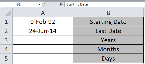
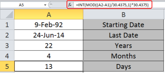
We need to find the years, month and days between the two given dates in A1 and A2 cell.

Write the formula in A3 cell to get the years between these two dates.

Formula

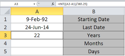
We can see the number of years in the A3 cell.

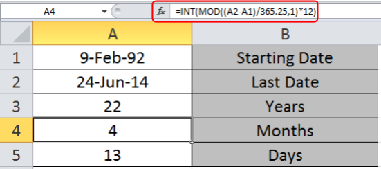
Now write the formula in A4  to get the months

=INT(MOD((A2-A1)/365.25,1)*12)

Use the Formula in A5 cell to get the days between the two dates.

=INT(MOD((A2-A1)/30.4375,1)*30.4375) 

Explanation:
As we know there are 12 months in a year and an average of 365.25 days in 4-year interval.
Here INT function returns the Integer part of the mathematical formulation part.

Here as you can see you get the number of Days, Months and Years between the two given dates.

Previously in Excel 2010 and Excel 2013, MS used to provide a date function named DATEDIF. It was found that it had some errors and was prone to give wrong outputs. This is why in Excel 2016 it is not promoted. But the function is still useful to calculate age. When you type this formula, no help or suggestion will be shown. You have to type it whole…

DATEDIF Syntax

Syntax:

=DATEDIF(date1,date2, “Y”)

“Y” will return the difference of years. At the place “Y” we can also write “M” or “D”.
As you must have guessed that “M” will return the difference in Months and “D” will return difference of Days.

These basic formulas and its uses can improve your time and efficiency using MS Excel 2016. Hope you understood how to count the number of days between the two given dates. You can perform these tasks in Excel 2013 and 2010. Please share your views on this topic below in the comment box. We will help you.

Related Articles:

How to Calculate years between dates in Excel

How to Add Years to a Date in Excel

How to Convert Date and Time from GMT to CST in Excel

How to Get days between dates in Excel

Popular Articles:

50 Excel Shortcut to Increase Your Productivity

How to use the VLOOKUP Function in Excel

How to use the COUNTIF function in Excel 2016

How to use the SUMIF Function in Excel