Calculate dates between excel and

If you manage multiple projects, you would have a need to know how many months have passed between two dates. Or, if you’re in the planning phase, you may need to know the same for the start and end date of a project.

There are multiple ways to calculate the number of months between two dates (all using different formulas).

In this tutorial, I will give you some formulas that you can use to get the number of months between two dates.

So let’s get started!

Using DATEDIF Function (Get Number of Completed Months Between Two Dates)

It’s unlikely that you will get the dates that have a perfect number of months. It’s more likely to be some number of months and some days that are covered by the two dates.

For example, between 1 Jan 2020 and 15 March 2020, there are 2 months and 15 days.

If you only want to calculate the total number of months between two dates, you can use the DATEDIF function.

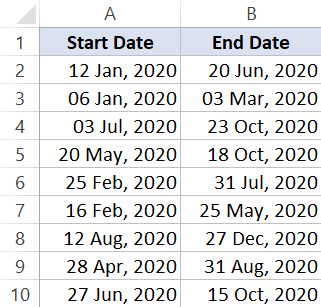
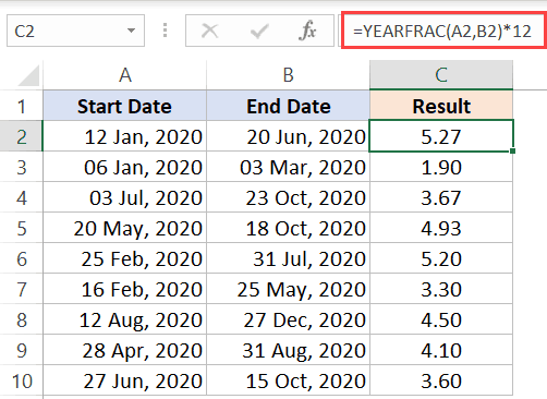
Suppose you have a dataset as shown below where you only want to get the total number of months (and not the days).

Below is the DATEDIF formula that will do that:

=DATEDIF(A2,B2,"M")

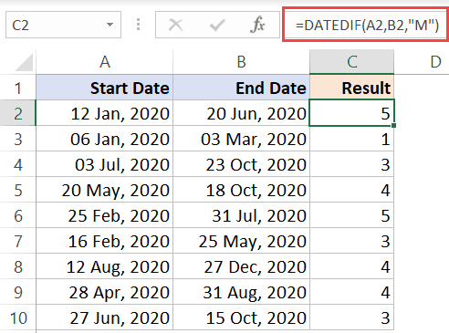
The above formula will give you only the total number of completed months between two dates.

DATEDIF is one of the few undocumented functions in Excel. When you type the =DATEDIF in a cell in Excel, you would not see any IntelliSense or any guidance on what arguments it can take. So, if you’re using DATEDIF in Excel, you need to know the syntax.

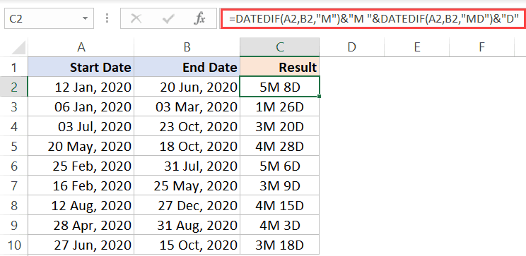
In case you want to get the total number of months as well as days between two dates, you can use the below formula:

=DATEDIF(A2,B2,"M")&"M "&DATEDIF(A2,B2,"MD")&"D"

Note: DATEDIF function will exclude the start date when counting the month numbers. For example, if you start a project on 01 Jan and it ends on 31 Jan, the DATEDIF function will give the number of months as 0 (as it doesn’t count the start date and according to it only 30 days in January have been covered)

Using YEARFRAC Function (Get Total Months Between Two Dates)

Another method to get the number of months between two specified dates is by using the YEARFRAC function.

The YEARFRAC function will take a start date and end date as input arguments and it will give you the number of years that have passed during these two dates.

Unlike the DATEDIF function, the YEARFRAC function will give you the values in decimal in case a year has not elapsed between the two dates.

For example, if my start date is 01 Jan 2020 and end date is 31 Jan 2o20, the result of the YEARFRAC function will be 0.833. Once you have the year value, you can get the month value by multiplying this with 12.

Suppose you have the dataset as shown below and you want to get the number of months between the start and end date.

Below is the formula that will do this:

=YEARFRAC(A2,B2)*12

This will give you the months in decimals.

In case you only want to get the number of complete months, you can wrap the above formula in INT (as shown below):

=INT(YEARFRAC(A2,B2)*12)

Another major difference between the DATEDIF function and YEARFRAC function is that the YEARFRAC function will consider the start date as a part of the month. For example, if the start date is 01 Jan and end date is 31 Jan, the result from the above formula would be 1

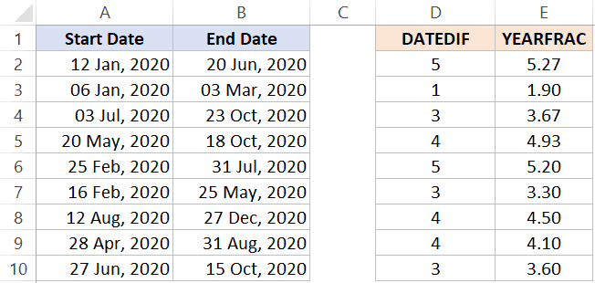
Below is a comparison of the results you get from DATEDIF and YEARFRAC.

Using the YEAR and MONTH Formula (Count All Months when the Project was Active)

If you want to know the total months that are covered between the start and end date, then you can use this method.

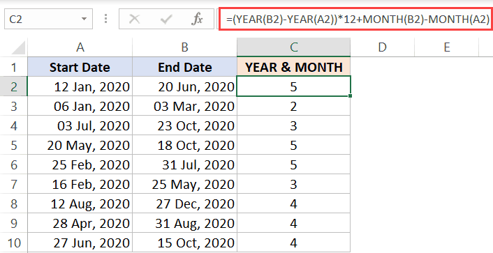
Suppose you have the dataset as shown below:

Below is the formula that will give you the number of months between the two dates:

=(YEAR(B2)-YEAR(A2))*12+MONTH(B2)-MONTH(A2)

This formula uses the YEAR function (which gives you the year number using the date) and the MONTH function (which gives you the month number using the date).

The above formula also completely ignores the month of the start date.

For example, if your project starts on 01 Jan and ends on 20 Feb, the formula shown below will give you the result as 1, as it completely ignores the start date month.

In case you want it to count the month of the start date as well, you can use the below formula:

=(YEAR(B2)-YEAR(A2))*12+(MONTH(B2)-MONTH(A2)+1)

You may want to use the above formula when you want to know-how in how many months was this project active (which means that it could count the month even if the project was active for only 2 days in the month).

So these are three different ways to calculate months between two dates in Excel. The method you choose would be based on what you intend to calculate (below is a quick summary):

• Use the DATEDIF function method if you want to get the total number of completed months in between two dates (it ignores the start date)
• Use the YEARFRAC method when you want to get the actual value of months elapsed between tow dates. It also gives the result in decimal (where the integer value represents the number of full months and decimal part represents the number of days)
• Use the YEAR and MONTH method when you want to know how many months are covered in between two dates (even when the duration between the start and the end date is only a few days)

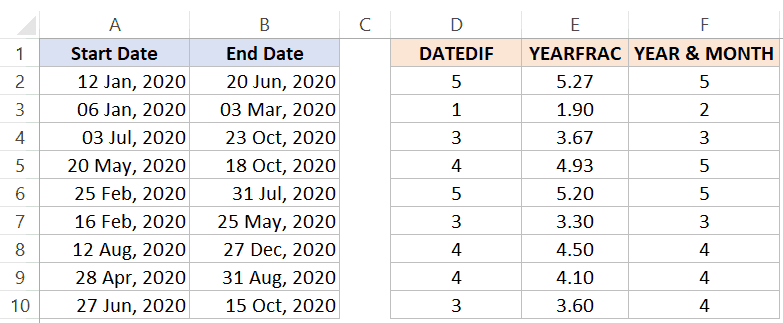
Below is how each formula covered in this tutorial will count the number of months between two dates:

Hope you found this Excel tutorial useful.

You may also like the following Excel tips and tutorials:

• How to Calculate the Number of Days Between Two Dates in Excel
• How to Remove Time from Date/Timestamp in Excel
• Convert Time to Decimal Number in Excel (Hours, Minutes, Seconds)
• How to Quickly Insert Date and Timestamp in Excel
• Convert Date to Text in Excel
• How to SUM values between two dates in Excel
• How to Add Months to Date in Excel
• How to Calculate Years of Service in Excel (Easy Formulas)
• How to Make an Interactive Calendar in Excel? (FREE Template)

This post will teach you how to calculate days, weeks, months and years between two dates in excel. How do I count the number of days, weeks, months and years between 2 dates in excel.

If you want to calculate the difference in days between two dates, you can use the DATEDIF function to create an excel formula as follows:

=DATEIF(B1,B2, "D")

This formula will calculate days between two dates in cell B1 and B2, then returns the value in days.

Calculate months between two dates

If you want to calculate the difference in months between tow dates, you can also use the DATEDIF function to create the following generic formula:

=DATEDIF(B1,B2,"M")

You should note that the third argument is “M” in the DATEDIF function. So this formula returns the value in months between two dates in excel.

Calculate years between two dates

You can also use the DATEDIF function to calculate the number of years between two dates in excel, just refer to the following excel formula based on the DATEDIF function:

=DATEDIF(B1,B2,"Y")

This formula returns the value in years.

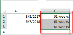
Calculate weeks between two dates

If you want to calculate the number of weeks between two dates, you just need to subtract start date from the end date and then the returned result is divided by 7. So you can write the below generic formula:

=(B2-B1)/7

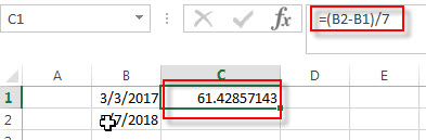
This formula will return a decimal number, you can change the number format as you need.

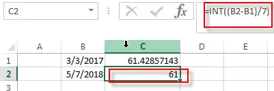
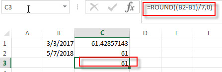
Or you can use the INT function to rounds down to the nearest whole number or use ROUND function to round to nearest whole number.

=INT((B2-B1)/7)

=ROUND((B2-B1)/7,0)

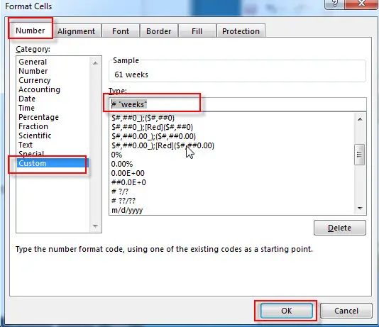
You may be want to display the word “week” before the week number in the cell, you can do it as following steps:

1# right-click on the selected cells, then select Format Cells

2# on the Number Tab, choose Custom under Category, then select # “weeks” type.

Calculate Years, Months and Days between two dates

If you want to determine how many years, months and days between two dates, you can use the DATEDIF function to create the following complex formula:

=DATEDIF(B1,B2,"Y") & " Years, " & DATEDIF(B1,B2,"YM") & " Months, " & DATEDIF(B1,B2,"MD") & " Days"

If you do not want to use the DATEDIF function, and you can also use the following formula to achieve the same result:

=INT((TODAY()-A1)/365.25) & ” years , ” & INT(MOD((TODAY()-A1)/365.25,1)*12) & ” months and ” & INT(MOD((TODAY()-A1)/30.4375,1)*30.4375) & ” days”

---

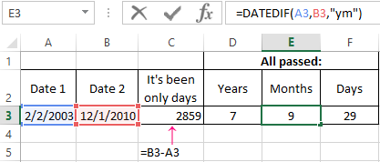
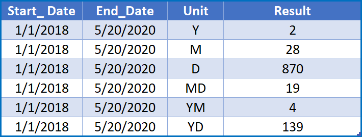
In this example, the goal is to output the time between a start date and an end date as a text string that lists years, months, and days separately. For example, given a start date of 1-Jan-2018 and end date of 1-Jul-2018, the result should be a string like this:

"1 years, 6 months, 0 days"

DATEDIF solution

The DATEDIF function is designed to calculate the difference between dates in years, months, and days. There are several variations available (e.g. time in months, time in months ignoring days and years, etc.) and these are set by the «unit» argument in the function. See this page on the DATEDIF function for a full list of available units.

In the example shown, we calculate years, months, and days separately, then «glue» the results together with concatenation. To get whole years, whole months, and days between the dates, we use DATEDIF like this, altering only the unit argument.

DATEDIF(B5,C5,"y") // years
DATEDIF(B5,C5,"ym") // months
DATEDIF(B5,C5,"md") // days

Because we want to create a string that appends the units to each number, we concatenate the number returned by DATEDIF to the unit name with the ampersand (&) operator like this:

DATEDIF(B5,C5,"y")&" years" // years string
DATEDIF(B5,C5,"ym")&" months" // months string
DATEDIF(B5,C5,"md")&" days" // days string

Finally, we need to extend the idea above to include spaces and commas and join everything together in one string:

=DATEDIF(B5,C5,"y")&" years, "&DATEDIF(B5,C5,"ym")&" months, " &DATEDIF(B5,C5,"md")&" days"

Implementing the LET function

The LET function (new in Excel 365) can simplify some formulas by making it possible to define and reuse variables. In order to use the LET function on this formula, we need to think about variables. The main purpose of variables is to define a useful name that can be reused elsewhere in the formula code. Looking at the formula, there are at least five opportunities to declare variables. The first two are the start date and the end date, which are reused throughout the formula. Once we assign values to start and end, we only need to refer to cell C5 and D5 one time. As a first step, we can add line breaks and then define variables for start and end like this:

=LET(
  start,B5,
  end,C5,
  DATEDIF(start,end,"y")&" years, "&
  DATEDIF(start,end,"ym")&" months, "&
  DATEDIF(start,end,"md")&" days"
)

Notice all instances of B5 and C5 in DATEDIF have been replaced by start and end. The result from this formula is the same as the original formula above, but the reference to B5 and C5 occurs only once. The start and end dates are then reused throughout the formula. This makes it easier to read the formula and helps reduce errors.

The next three opportunities for variables are the results from DATEDIF for years, months, and days. If we assign these values to named variables, we can more easily combine them later in different ways, which becomes more useful in the extended version of the formula explained below. Here is the formula updated to include new variables for years, months, and days:

=LET(
  start,B5,
  end,C5,
  years,DATEDIF(start,end,"y"),
  months,DATEDIF(start,end,"ym"),
  days,DATEDIF(start,end,"md"),
  years&" years,"&months &" months," &days &" days"
)

Notice we have assigned results from DATEDIF to the variables years, months, and days, and these values are concatenated together in the last line inside the LET function. With the LET function, the last argument is the calculation or value that returns a final result.

Getting fancy with LET

Once we have the basic LET version working, we can easily extend the formula to do more complex processing, without redundantly running the same calculations over again. For example, one thing we might want to do is make the units plural or singular depending on the actual unit number.  The formula below adds three new variables: ys, ms, and ds to hold the strings associated with each unit:

=LET(
  start,B5,
  end,C5,
  years,DATEDIF(start,end,"y"),
  months,DATEDIF(start,end,"ym"),
  days,DATEDIF(start,end,"md"),
  ys,years&" year"&IF(years<>1,"s",""),
  ms,months&" month"&IF(months<>1,"s",""),
  ds,days&" day"&IF(days<>1,"s",""),
  ys&", "&ms&", "&ds
)

The strings start out singular (i.e. » year» not «years»). Then we use the IF function to conditionally tack on an «s» only when the number is not 1. If the number is 1, IF returns an empty string («») and the unit name remains singular. Because we add the unit name to the unit number when we define ys, ms, and ds, the last step inside LET is simpler; we only need to concatenate the units with a comma and space.

See more details about the LET function here. Also, see the Detailed LET function example for another explanation of converting an existing formula to use LET.

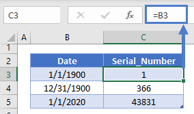
The date and time in Excel — there are numbers, formatted in a special way. The date is the integer part of the number, and the time (hours and minutes) is the fractional part.

By default, the number 1 corresponds to the date of 01. 01. 1900 — that is, each date — is the number of days passed from 01. 01. 1900. In this lesson, we will take a closer look at the dates, and in the next lessons – the time.



How in Excel to calculate the days between dates?

Since the date is a number, it means that you can conduct mathematical computing and settlement operations. To count the number of days between two Excel dates does not present any special problems. For a visual example, we first perform the addition, and then subtraction of dates. For this:

1. On a blank sheet in the cell A1 you need to enter the current date by pressing CTRL +.
2. In the cell A2 you need to enter an intermediate period in days, for example, 127.
3. In the cell A3 you need to enter the formula: = A1 + A2.

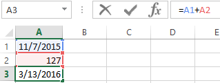
Note that the «Date» format was automatically assigned to the cell A3. It’s not difficult to guess, to calculate the difference in dates in Excel, you need to take away the highest date from the newest date. In the cell B1 you need to enter the formula: A3 — A1. Accordingly, we get the number of days between these two dates.



The calculating age by date of birth in Excel

Now we will learn how to calculate the age by date of birth:

1. In the new sheet in the cells A1: A3, you need to enter the dates: 18. 04. 1985; 17. 08. 1977; 08. 12. 1992.
2. In the cells B1 : B3, you need to put the current date.
3. Now you need to use the function to convert the number of days to the number of years. To do this, you need to enter by manually the following value in the range C1:C3: = DATEDIF(A1; B1; «y»).

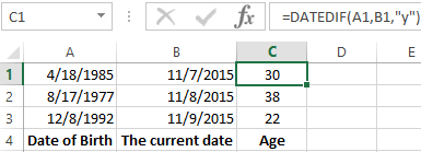
Thus, the application of the function allowed us to accurately calculate the age by date of birth in Excel.

Attention! To transform days into years, there is not enough of the formula: Moreover, even if we know that 1 day = 0.0027397260273973 of the year, the formula: =(B1-A1)*0.0027397260273973 will not give us the exact result either.

Days in the years the most accurately to convert the function: = DATEDIF(). You will not find it in the list of the function wizard (SHIFT+F3), but if you simply to enter it into the formula line, it will work.

The DATEDIF function supports to the several parameters:

Option	Description
«d»	Count of full days;
«m»	Count of full months;
«y»	Count of full years;
«ym»	Count of full months without years;
«md»	Count of days without months and years;
«yd»	Count of days without years.

Let’s illustrate the example of using several parameters:

Attention! That the function: = DATEDIF() worked without errors, make sure that the start date was older than the end date.

The insertion of the date in the Excel cell

The purpose of this lesson is an example of mathematical operations with dates. Also, we’ll make sure that for Excel, the date data type is a number.

You need to fill in the table with dates, as shown in the picture:

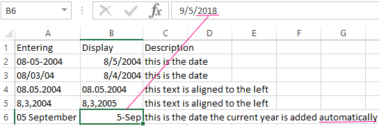
There are different ways of entering dates: in the column A there is input method, and in column B there is the display result.

Note that the default format cell is «General», the dates as well as the number are aligned on the right side, and the text on the left one. The value in the cell B4 is recognized by the program as text.

In the cell B7 Excel has assigned by itself to the current year (now is the 2015-th) by default. This is visible when displaying the contents of cells in the formula bar. Notice how the value was originally entered in A7.

The calculating of the Excel date

On the blank sheet in the cells A1 and C1 you need to enter 01. 01. 1900, and in the cells A2 and C2 is 01. 01. 1901. Now we change the format of the cells to «numeric» in the selected range C1:C2. To do this, you can press CTRL + SHIFT + 1.

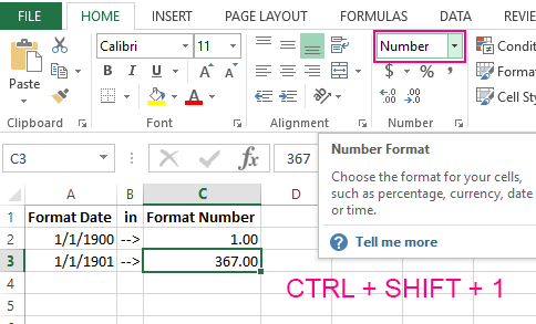
C1 contains now the number 1, and C2 — 367. That is, one leap year (366 days) now and one day passed.

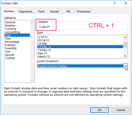
The way to display the date can be set using the «Format Cells» dialog box. To call it, press: CTRL + 1. On the «Number» tab, you need to select «Category:» — «Date». In the «Type:» section displays the most popular formats for displaying dates.

Download examples calculate date in Excel

Read also: The functions for working with dates in Excel

In the next lesson, we will work with the time and the periods of the day on ready-made examples.

This tutorial will teach you how to calculate the number of days between two dates in Excel and Google Sheets.

Excel Subtract Dates

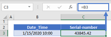
In Excel, dates are stored as serial numbers:

This allows you to subtract dates from one another to calculate the number of days between them:

=C3-B3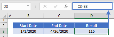

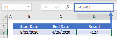
If the End Date is before the Start Date you’ll receive a negative answer:

If you need the absolute number of days between the dates, use the ABS Function to return the absolute value:

=ABS(C3-B3)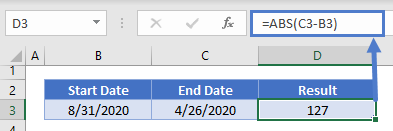

Subtract Dates with Times

In Excel, times are stored as decimal values. A decimal value attached to a serial number represents a Date & Time:

If you subtract a Date and Time from another Date and Time. You’ll receive a Date and Time answer (number of days, hours, minutes, seconds between the two dates):

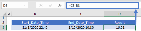
Notice how the number of days between the dates is *3*, but the decimal value is *2.2* because of the time difference?  This may or may not be what you want.

Instead, you could use the TRUNC Function to find the difference between the dates:

=TRUNC(C3)-TRUNC(B3)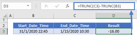

But you can also use the DAYS or DATEDIF functions for an easier calculation…

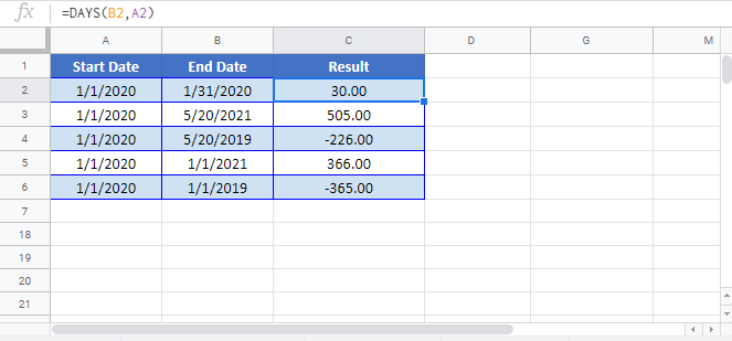
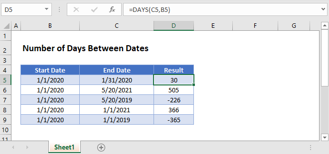
DAYS Function – Calculate Difference Between Dates

The DAYS Function calculates the number of days between dates, ignoring times.

=DAYS(C3,B3)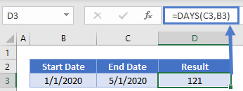

The DAYS Function will return negative values, so you may want to use the ABS Function for the absolute number of days between dates:

=ABS(DAYS(C3,B3))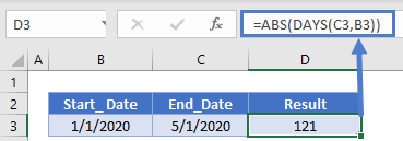

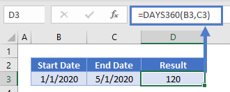
DAYS360 Function

The DAYS360 Function works the same as the DAYS Function, except it assumes a 360-day year where each month has 30 days. Notice the difference in calculations:

=DAYS360(B3,C3)

DATEDIF Function – Number of Days Between Dates

The DATEDIF Function can be used to calculate the date difference in various units of measurement, including days, weeks, months, and years.

To use the DATEDIF Function to calculate the number of days between dates set the unit of measurement to “d” for days:

=DATEDIF(B3,C3,"d")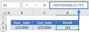

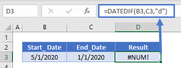
Unlike the other methods, the DATEDIF Function will not work if the end_date is before the start_date, instead it will throw a #NUM! error.

To calculate difference between dates with other units of measurement use this table as a reference:

Calculate Number of Days Between Today and Another Date

To calculate the number of days from Today to another date, use the same logic with the TODAY Function for one of the dates.

This will calculate the number of days since a date:

=DAYS(TODAY(),B3)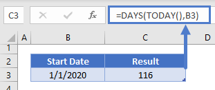

This will calculate the number of days until a date:

=DAYS(B3,TODAY())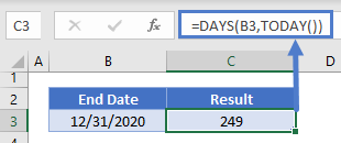

Calculate Working (Business) Days Between Dates

The NETWORKDAYS Function allows you to calculate the number of working (business) days between two dates:

=NETWORKDAYS(B4,C4)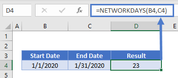

By default, NETWORKDAYS will ignore all holidays. However you can use a 3rd optional argument to define a range of holidays:

=NETWORKDAYS(B4,C4,F3:F4)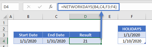

Google Sheets – Days Between Dates

All of the above examples work exactly the same in Google Sheets as in Excel.