Cagr formula for excel

There’s no CAGR function in Excel. However, simply use the RRI function in Excel to calculate the compound annual growth rate (CAGR) of an investment over a period of years.

1. The RRI function below calculates the CAGR of an investment. The answer is 8%.

Note: the RRI function has three arguments (number of years = 5, start = 100, end = 147).

2. The CAGR measures the growth of an investment as if it had grown at a steady rate on an annually compounded basis. We can check this.

which is the same as:

Note: again, number of years or n = 5, start = 100, end = 147, CAGR = 8%.

3. Knowing this, we can easily create a CAGR formula that calculates the compound annual growth rate of an investment in Excel.

A2 = A1 * (1 + CAGR)ⁿ

end = start * (1 + CAGR)ⁿ

end/start = (1 + CAGR)ⁿ

(end/start)^1/n = (1 + CAGR)

CAGR = (end/start)^1/n — 1

4. The CAGR formula below does the trick.

Note: in other words, to calculate the CAGR of an investment in Excel, divide the value of the investment at the end by the value of the investment at the start. Next, raise this result to the power of 1 divided by the number of years. Finally, subtract 1 from this result.

Источник

Compound Annual Growth Rate, CAGR, is your rate of return for an investment over a specific period.

Calculating CAGR by hand is a rather involved process, so below we’ll go over how you can quickly calculate CAGR in Excel.

CAGR Excel Formula

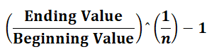
The formula for calculating CAGR in Excel is:

=(End Value/Beginning Value) ^ (1/Number of Years) — 1

The equation uses three different values:

End value, which is the amount of money you’ll have after the period has passed.
Beginning value, which is the amount of money you began with.
Number of years, which is the total number of years that have passed.

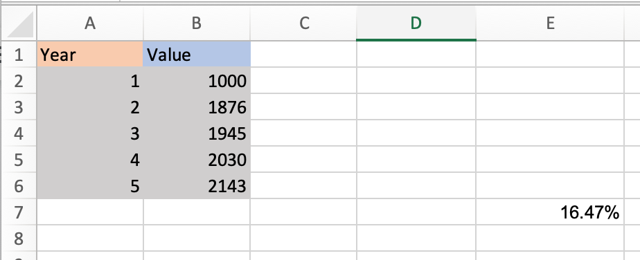
Below we’ll go over an example of how to calculate CAGR for a five years time frame in Excel using the sample data set shown below:

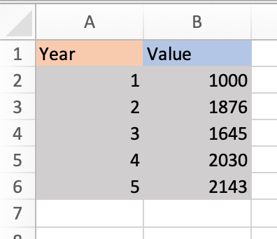
1. Identify the numbers you’ll use in your equation. Using the sample data set above,

The end value is 2143 (in cell B6).
The beginning value is 1000 (in cell B2).
The number of years is 5 (in cell A6).

2. Input your values into the formula.

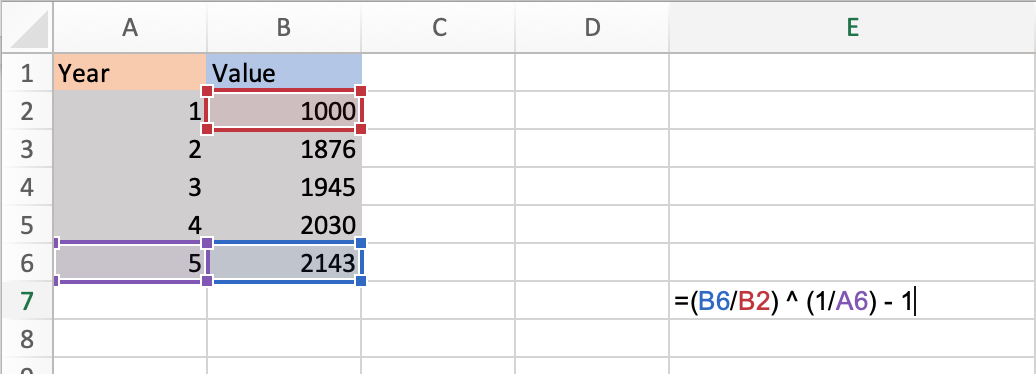
Excel offers many shortcuts, so you can simply input the cell numbers that contain each of your values into the equation. Using the sample data set above, the equation would be

=(B6/B2) ^ (1/A6) — 1

This is what it looks like in my Excel sheet:

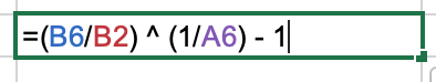
Note that the equation changes color to correspond with the cells you’re using, so you can look back and check that your inputs are correct before running the equation.

You can also enter actual values into the formula instead of cell numbers. The equation would then look like this:

=(2143/1000) ^ (1/5) — 1

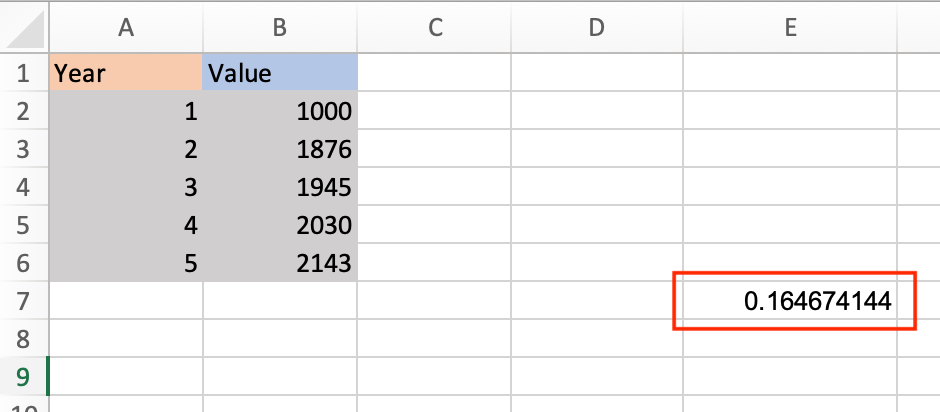
3. Once you’ve entered your values, click enter and run the equation. Your result will appear in the cell containing the equation, as shown in the image below.

CAGR Formula in Excel as a Percentage

Your default result will be shown as a decimal. To view it as a percentage, right-click on the cell your result is in, select Format Cells and then Percentage in the dialogue box.

Your result will be converted to a percentage, as shown in the image below.

Now let’s go over a shortcut for calculating CAGR in Excel using the Rate function.

How To Calculate CAGR Using RATE Function

The RATE function helps you calculate the interest rate on an investment over a period of time.The formula for calculating CAGR is:

=RATE(nper,, pv, fv)

nper is the total number of periods in the time frame you’re measuring for. Since you’re calculating annual growth rate, this would be 12.
pv is the present value of your investment (must always be represented as a negative)
fv is future value.

Note that the standard RATE equation includes more variables, but you only need the above three to calculate your CAGR.

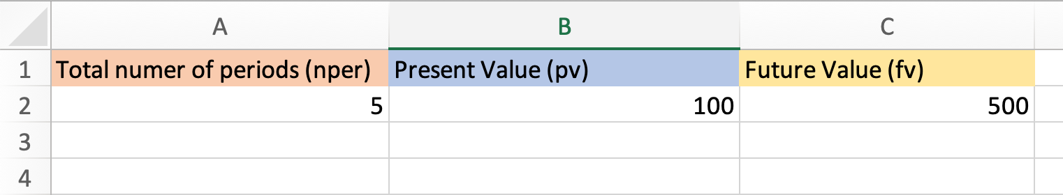
Let’s run an equation using the sample table below where nperi is 12, pv is 100, and fv is 500.

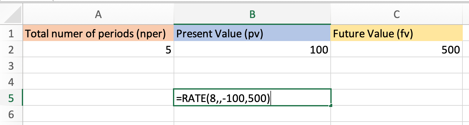
1. In your sheet, select the cell that you want to contain your CAGR. I selected cell B5.

2. Enter the RATE formula and input your numbers. Note that you always need to express your present value as a negative, or you’ll receive an error message.

This is what my formula looks like.

Note that you can also simply enter the cell numbers that your values are in. With my sample table the formula would look like this:

=RATE(A2,,-B2,C2)

3. Click enter and run your equation. Using the sample data, my CAGR is 14%.

Now you know how to quickly and easily calculate your CAGR in Excel, no hand calculations required.

Источник

CAGR, or compound annual growth rate, is a method to calculate the growth rate of a particular amount annually. Unfortunately, we do not have any inbuilt formula in Excel to calculate CAGR by default. So instead, we make categories in tables, and in tables, we apply the following formula to calculate CAGR: (Ending Balance/Starting Balance)˄(1/Number of Years) – 1.

For example, suppose you have a company’s financial report and need to know the annual growth rate of an investment over a given period. You may estimate a year-to-year growth using a formula in your Excel worksheets without hand calculations.

CAGR Formula in Excel (Compound Annual Growth Rate)

The CAGR formula in Excel is the function that is responsible for returning the CAGR value, the Compound Annual Growth Rate value, from the supplied set of values. If you are into financial analysis or planningFinancial planning and analysis (FP&A) is budgeting, analyzing, and forecasting the financial data to align with its financial objectives and support its strategic decisions. It helps investors to know if the company is stable and profitable for investment.read more, you will need to calculate the compound annual growth rate in Excel value in Excel spreadsheets.

The CAGR formula in Excel measures the value of return on an investment calculated over a certain period. The compound annual growth rate formula in Excel is often used in Excel spreadsheets by financial analysts, business owners, or investment managersAn investment manager manages the investments of others using several strategies to generate a higher return for them and grow their assets. They are sometimes also referred to as portfolio managers, asset managers, or wealth managers. They may also be considered financial advisors in some cases, but they are typically less involved in the sales aspect.read more, which helps them identify how much their business has developed or compare revenue growth with the competitor companies. With the help of CAGR, it can be seen how much constant growth rate the investment should return annually. In reality, the growth rate should vary from year to year.

For example, if you bought gold in 2010 worth $200 and $500 in 2018, CAGR is how this investment has grown yearly.

where,

Ending Value = Investment’s ending value
Starting Value = Investment’s starting value
n = number of investment periods (months, years, etc.)

Return Value:

The return value will be numeric, which we can convert into a percentage because the CAGR is effective in percentage form.

CAGR Formula in Excel (Compound Annual Growth Rate)
- How to Use CAGR Formula in Excel with Examples?
  - #1 – Basic Method
  - #2 – Using the Power Function
  - #3 – Using the RATE Function
  - #4 – Using the IRR Function
- CAGR Formula Errors
- Things to Remember
- Recommended Articles

How to Use CAGR Formula in Excel with Examples?

Let us understand how to use the CAGR formula in Excel with examples.

You can download this CAGR Formula Excel Template here – CAGR Formula Excel Template

#1 – Basic Method

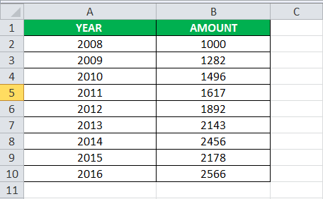
Let us consider the Excel spreadsheet below. Look at the data.

Below are the steps of the CAGR formula in Excel: –

The above spreadsheet shows where column A has been categorized as “YEAR,” and column B has “AMOUNT.”

In column “YEAR,” the value starts from the A2 cell and ends at the A10 cell.

Again in the column “AMOUNT,” the value starts at the B2 cell and ends at the B10 cell.

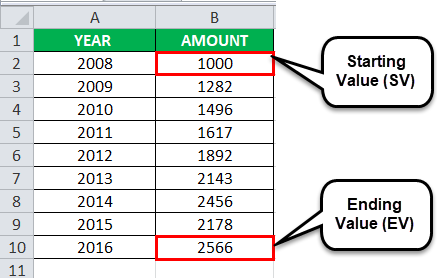
Therefore, we can see that the investment’s Starting Value (SV) is the B2 cell and the investment’s Ending Value (EV) is the B10 cell.
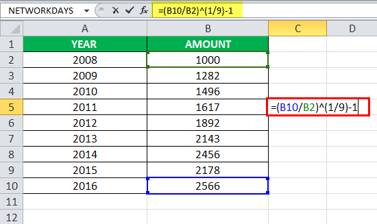
We have the values, which we can put in Excel’s Compound Annual Growth Rate (CAGR) formula. However, to successfully do it in an Excel spreadsheet, we have to select any of the cells of the C column and type the formula as given below:

=(B10/B2)^(1/9)-1

In the above compound annual growth rate in Excel example, the ending value is B10, the beginning value is B2, and the number of periods is 9. You may see the screenshot below.
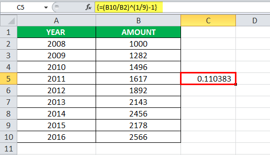
Now press the “Enter” key. We will get the CAGR (Compound Annual Growth Rate) value result inside the cell where we input the formula. In the above example, the CAGR value will be 0.110383. The return value is just the evaluation of the CAGR formula in Excel with the values which have been described above. Consider the screenshot below.
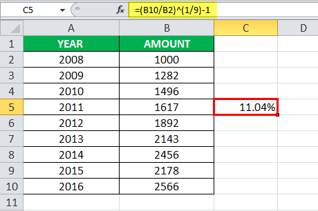
Note that Compound Annual Growth Rate in Excel is always represented in the form of percentages in the financial analysis field. To get the percentage, we must select the cell where the CAGR value is present and change the cell format from ‘General’ to ‘Percentage.’ The percentage value of CAGR (Compound Annual Growth Rate) in the above example is 11.04%. We can see the screenshot below.

The above steps show how you calculate the Compound Annual Growth Rate in Excel (CAGR) spreadsheets.

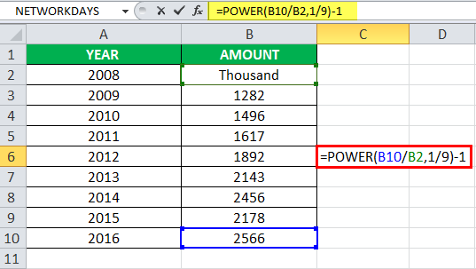
#2 – Using the Power Function

You can also use the POWER formula in ExcelPOWER function calculates the power of a given number or base. To use this function you can use the keyword =POWER( in a cell and provide two arguments one as number and another as power.read more to find the CAGR value in your Excel spreadsheet. The formula will be “=POWER (Ending Value/Beginning Value, 1/9)-1”. We can see that the POWER function replaces the ˆ, which was used in the traditional CAGR formula in Excel. Using the POWER function in the above Excel spreadsheet, using the conventional method to find the CAGR value, the result will be 0.110383 or 11.03%. Consider the screenshot below.

#3 – Using the RATE Function

It is a much lesser-used method for calculating the CAGR (Compound Annual Growth Rate) value or percentage but cleanly. The syntax of the RATE function in ExcelRate function in excel is used to calculate the rate levied on a period of a loan. The required inputs for this function are number of payment periods, pmt, present value and future value.read more can seem a bit complicated, but if we know the terms well, it will not be too hard. The syntax of the RATE function is given below: –

=RATE (nper, pmt, pv, [fv], [type], [guess])

Let us now have an explanation of the above-given terms.

nper – (required) This is the total number of payments made in the specific period.
pmt – (required) This is the value of a payment made in each period.
pv – (required) This is the present value.
fv – (optional) This is the future value.
type – This means when the payments are due. The value is either 0 or 1. 0 represents the payment that has been due in the beginning, and 1 means that the payment has been expected at the end of the period.

#4 – Using the IRR Function

IRRInternal rate of return (IRR) is the discount rate that sets the net present value of all future cash flow from a project to zero. It compares and selects the best project, wherein a project with an IRR over and above the minimum acceptable return (hurdle rate) is selected.read more is the abbreviation of the Internal Rate of Return. The IRR method is helpful when finding the CAGR (Compound Annual Growth Rate) value for different value payments made during a specific period. The syntax of the IRR function in excelThe internal rate of return, or IRR, calculates the profit generated by a financial investment. IRR is a built-in function in Excel that calculates the IRR using a range of values as an input and an estimate value as the second input.read more is “=IRR (values, [guess]).” Values mean the entire range of numbers representing the cash flows. This section must contain one positive and one negative value. [Guess] in an optional argument in the syntax, which means your guess at what the return rate might be.

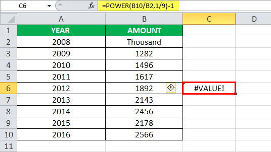
CAGR Formula Errors

If you get any error from the CAGR formula Excel, this is likely the #VALUE! Error.

#VALUE!Error – This error will occur if any supplied arguments are not valid values recognized by Excel.

Things to Remember

The Microsoft Excel CAGR formula returns the CAGR value, i.e., the Compound Annual Growth Rate in Excel from the supplied values set.
CAGR measures the return value on an investment, which is calculated over a certain period.
Using the Compound Annual Growth Rate formulaThe Growth rate formula is used to calculate the annual growth of the company for a particular period. It is computed by subtracting the prior value from the current value and dividing the result by the prior value.read more in Excel, it can be seen how much constant growth rate should the investment return on an annual basis.
If you get any error from the Excel CAGR formula, this is likely the #VALUE! Error.

Как использовать формулу CAGR в Excel с примерами?

Давайте разберемся, как использовать формулу CAGR в Excel с примерами.

.free_excel_div{фон:#d9d9d9;размер шрифта:16px;радиус границы:7px;позиция:относительная;margin:30px;padding:25px 25px 25px 45px}.free_excel_div:before{content:»»;фон:url(центр центр без повтора #207245;ширина:70px;высота:70px;позиция:абсолютная;верх:50%;margin-top:-35px;слева:-35px;граница:5px сплошная #fff;граница-радиус:50%} Вы можете скачать этот шаблон формулы CAGR Excel здесь — Формула CAGR Excel Шаблон

#1 – Основной метод

Давайте рассмотрим электронную таблицу Excel ниже. Посмотрите на данные.

Ниже приведены шаги формулы CAGR в Excel: –

В приведенной выше электронной таблице показано, где столбец А был отнесен к категории «ГОД», а столбец Б — к «СУММА».
В столбце «ГОД» значение начинается с ячейки A2 и заканчивается ячейкой A10.

Снова в столбце «СУММА» значение начинается с ячейки B2 и заканчивается ячейкой B10.

Таким образом, мы видим, что начальная стоимость инвестиции (SV) — это ячейка B2, а конечная стоимость инвестиции (EV) — ячейка B10.
У нас есть значения, которые мы можем поместить в формулу Excel Compound Annual Growth Rate (CAGR). Однако, чтобы успешно сделать это в электронной таблице Excel, мы должны выбрать любую из ячеек столбца C и ввести формулу, как показано ниже:
=(В10/В2)^(1/9)-1

В приведенном выше сложном годовом темпе роста в примере Excel конечное значение — B10, начальное значение — B2, а количество периодов — 9. Вы можете увидеть снимок экрана ниже.
Теперь нажмите клавишу «Ввод». Мы получим результат значения CAGR (сложный годовой темп роста) внутри ячейки, в которую мы вводим формулу. В приведенном выше примере значение CAGR будет равно 0,110383. Возвращаемое значение — это просто оценка формулы CAGR в Excel со значениями, которые были описаны выше. Рассмотрим скриншот ниже.
Обратите внимание, что совокупный годовой темп роста в Excel всегда представлен в виде процентов в поле финансового анализа. Чтобы получить процент, мы должны выбрать ячейку, в которой присутствует значение CAGR, и изменить формат ячейки с «Общий» на «Процент». Процентное значение CAGR (сложный годовой темп роста) в приведенном выше примере составляет 11,04%. Мы можем видеть скриншот ниже.

Приведенные выше шаги показывают, как рассчитать совокупный годовой темп роста в электронных таблицах Excel (CAGR).

#2 – Использование функции мощности

Вы также можете использовать формулу POWER в ExcelФормула POWER В ExcelPOWER функция вычисляет степень данного числа или основания. Чтобы использовать эту функцию, вы можете использовать ключевое слово =МОЩНОСТЬ( в ячейке и указать два аргумента, один как число, а другой как мощность. Узнайте больше, чтобы найти значение CAGR в электронной таблице Excel. Формула будет «=МОЩНОСТЬ (конечное значение/ Начальное значение, 1/9)-1″. Мы видим, что функция СТЕПЕНЬ заменяет ˆ, которая использовалась в традиционной формуле CAGR в Excel. Используя функцию СТЕПЕНЬ в приведенной выше электронной таблице Excel, используя обычный метод, чтобы найти CAGR, результат будет 0,110383 или 11,03%.Рассмотрите скриншот ниже.

#3 – Использование функции RATE

Это гораздо менее используемый метод для расчета значения или процента CAGR (Совокупный годовой темп роста), но чистый. Синтаксис функции СТАВКА в ExcelФункция СТАВКА В ExcelФункция СТАВКА в Excel используется для расчета ставки, взимаемой за период кредита. Необходимыми входными данными для этой функции являются количество периодов оплаты, PMT, текущая стоимость и будущая стоимость. Читать больше может показаться немного сложным, но если мы хорошо знаем условия, это не будет слишком сложно. Синтаксис функции RATE приведен ниже: –

= СТАВКА (кпер, плт, пв, [fv], [type], [guess])

Приступим теперь к объяснению вышеприведенных терминов.

например – (обязательно) Это общее количество платежей, совершенных за определенный период.
пмт – (обязательно) Это значение платежа, сделанного в каждом периоде.
пв – (обязательно) Это текущая стоимость.
фв – (необязательно) Это будущая стоимость.
тип – Это означает, когда должны быть произведены платежи. Значение равно 0 или 1. 0 представляет платеж, который должен был быть произведен в начале, а 1 означает, что платеж ожидается в конце периода.

#4 – Использование функции IRR

IRRIRRВнутренняя норма доходности (IRR) — это ставка дисконтирования, которая устанавливает нулевую чистую текущую стоимость всех будущих денежных потоков от проекта. Он сравнивает и выбирает лучший проект, при этом выбирается проект с IRR, превышающим минимально допустимую доходность (барьерную ставку). Читать далее — это сокращение от внутренней нормы доходности. Метод IRR полезен при нахождении значения CAGR (Совокупный годовой темп роста) для платежей различной стоимости, сделанных в течение определенного периода. Синтаксис функции IRR в ExcelСинтаксис функции IRR в ExcelВнутренняя норма прибыли, или IRR, рассчитывает прибыль, полученную от финансовых инвестиций. IRR — это встроенная в Excel функция, которая вычисляет IRR, используя диапазон значений в качестве входных данных и оценочное значение в качестве второго входного значения. Подробнее: «= IRR (значения, [guess])». Значения означают весь диапазон чисел, представляющих денежные потоки. Этот раздел должен содержать одно положительное и одно отрицательное значение. [Guess] в необязательном аргументе в синтаксисе, что означает ваше предположение о том, какой может быть скорость возврата.

Ошибки формулы CAGR

Если вы получаете какую-либо ошибку в формуле CAGR Excel, скорее всего, это ошибка #ЗНАЧ! Ошибка.

#ЗНАЧ!Ошибка. Эта ошибка возникает, если какие-либо предоставленные аргументы не являются допустимыми значениями, распознаваемыми Excel.

То, что нужно запомнить

Формула CAGR Microsoft Excel возвращает значение CAGR, т. е. совокупный годовой темп роста в Excel из предоставленного набора значений.
CAGR измеряет доходность инвестиций, которая рассчитывается за определенный период.
Использование формулы сложного годового темпа ростаФормула темпа ростаФормула темпа роста используется для расчета годового роста компании за определенный период. Он вычисляется путем вычитания предшествующего значения из текущего значения и деления результата на предыдущее значение. Подробнее в Excel можно увидеть, насколько постоянный темп роста должен возвращать инвестиции на ежегодной основе.
Если вы получите какую-либо ошибку в формуле Excel CAGR, скорее всего, это ошибка #ЗНАЧ! Ошибка.

Compound Annual Growth Rate (CAGR)

CAGR stands for Compound Annual Growth Rate. CAGR is the year-over-year average growth rate over a period of time. In other words, CAGR represents what the return would have been assuming a constant growth rate over the period. In actuality, the growth rate should vary from year to year.

The CAGR Formula

From Investopedia, Compound Annual Growth Rate ( CAGR ) is calculated as:

=(Ending Value/Begining Value)^(1/# of years) -1

Restated:

=(FV/PV)^(1/n) -1

where FV = Future Value, PV = Present Value, and n = number of periods.

Calculate CAGR in Excel

FV, PV, N

If you have FV, PV, and n, simply plug them into the standard CAGR equation to solve for CAGR.

=(B5/C5)^(1/D5)-1 Result: 20%

The Rate Function

You can also use Excel's Rate Function:

= RATE (nper, pmt, pv, [fv], [type], [guess])

nper - The total number of payment periods
pmt - The payment amount. Payment must remain constant.
pv - The present value.
fv - [optional] The future value, or cash balance you want to be attained after the last pmt. 0 if omitted.
type - [optional] The payment type. 1 for beginning of period. 0 for end of period (default if omitted).
guess - [optional] Your guess for what the rate will be. 10% if omitted.

=RATE(B5,C5,D5)
Result: 12%

You can only use the RATE Function if the cash flows happen on a periodic basis, meaning the cash flows must happen at the same time annually, semi-annually, quarterly, etc. If the cash flows are not periodic, use the XIRR Function to calculate CAGR instead.

The XIRR Function

For non-periodic cash flows, use the XIRR Function to calculate CAGR. When using the XIRR Function, you create two columns. The first column contains the cash flows. The second column contains the cash flows' corresponding dates.

=XIRR(B5:B8,C5:C8,0.25)
Result: 24%

The IRR Function

Instead of using the Rate Function, you can use the IRR Function to calculate the CAGR for periodic cash flows. The IRR Function works the same as the XIRR Function, except you don't need to specify dates.

=IRR(B5:B10,.25)
Result: 8%

Apply Percentage Formatting to CAGR

After you finish calculating CAGR, your result may appear as a decimal: ex. .103. To convert your answer into a percentage (10.3%), you need to change the Number Formatting to percentage:

Return the Formula Examples Page.

Источник

CAGR Excel Formula

CAGR Formula in Excel as a Percentage

How To Calculate CAGR Using RATE Function

CAGR Formula in Excel (Compound Annual Growth Rate)

Table of contents

How to Use CAGR Formula in Excel with Examples?

#1 – Basic Method

#2 – Using the Power Function

#3 – Using the RATE Function

#4 – Using the IRR Function

CAGR Formula Errors

Things to Remember

Recommended Articles

Как использовать формулу CAGR в Excel с примерами?

Ошибки формулы CAGR

То, что нужно запомнить

Рекомендуемые статьи

Compound Annual Growth Rate (CAGR)

The CAGR Formula

Calculate CAGR in Excel

FV, PV, N

The Rate Function

The XIRR Function

The IRR Function

Apply Percentage Formatting to CAGR