
Содержание
- Using IF with AND, OR and NOT functions
- Examples
- Using AND, OR and NOT with Conditional Formatting
- Need more help?
- See also
- Function IF in Excel with a few examples of conditions
- The syntax of the function «IF» with one condition
- The function IF in Excel with multiple conditions
- Enhanced functionality with the help of the operators «AND» and «OR»
- How to compare data in two tables
- Excel Commands
- List of Top 10 Commands in Excel
- #1 VLOOKUP Function to Fetch Data
- #2 IF Condition to Do Logical Test
- #3 CONCATENATE Function to Combine Two or More Values
- #4 Count Only Numerical Values
- #5 Count All Values
- #6 Count Based on Condition
- #7 Count Number of Characters in the Cell
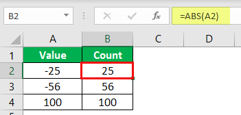
- #8 Convert Negative Value to Positive Value
- #9 Convert All Characters to UPPERCASE Values
- #10 Find Maximum and Minimum Values
- Things to Remember
- Recommended Articles
Using IF with AND, OR and NOT functions
The IF function allows you to make a logical comparison between a value and what you expect by testing for a condition and returning a result if that condition is True or False.
=IF(Something is True, then do something, otherwise do something else)
But what if you need to test multiple conditions, where let’s say all conditions need to be True or False ( AND), or only one condition needs to be True or False ( OR), or if you want to check if a condition does NOT meet your criteria? All 3 functions can be used on their own, but it’s much more common to see them paired with IF functions.
Use the IF function along with AND, OR and NOT to perform multiple evaluations if conditions are True or False.
IF(AND()) — IF(AND(logical1, [logical2], . ), value_if_true, [value_if_false]))
IF(OR()) — IF(OR(logical1, [logical2], . ), value_if_true, [value_if_false]))
IF(NOT()) — IF(NOT(logical1), value_if_true, [value_if_false]))
The condition you want to test.
The value that you want returned if the result of logical_test is TRUE.
The value that you want returned if the result of logical_test is FALSE.
Here are overviews of how to structure AND, OR and NOT functions individually. When you combine each one of them with an IF statement, they read like this:
AND – =IF(AND(Something is True, Something else is True), Value if True, Value if False)
OR – =IF(OR(Something is True, Something else is True), Value if True, Value if False)
NOT – =IF(NOT(Something is True), Value if True, Value if False)
Examples
Following are examples of some common nested IF(AND()), IF(OR()) and IF(NOT()) statements. The AND and OR functions can support up to 255 individual conditions, but it’s not good practice to use more than a few because complex, nested formulas can get very difficult to build, test and maintain. The NOT function only takes one condition.

Here are the formulas spelled out according to their logic:
=IF(AND(A2>0,B2 0,B4 50),TRUE,FALSE)
IF A6 (25) is NOT greater than 50, then return TRUE, otherwise return FALSE. In this case 25 is not greater than 50, so the formula returns TRUE.
IF A7 (“Blue”) is NOT equal to “Red”, then return TRUE, otherwise return FALSE.
Note that all of the examples have a closing parenthesis after their respective conditions are entered. The remaining True/False arguments are then left as part of the outer IF statement. You can also substitute Text or Numeric values for the TRUE/FALSE values to be returned in the examples.
Here are some examples of using AND, OR and NOT to evaluate dates.

Here are the formulas spelled out according to their logic:
IF A2 is greater than B2, return TRUE, otherwise return FALSE. 03/12/14 is greater than 01/01/14, so the formula returns TRUE.
=IF(AND(A3>B2,A3 B2,A4 B2),TRUE,FALSE)
IF A5 is not greater than B2, then return TRUE, otherwise return FALSE. In this case, A5 is greater than B2, so the formula returns FALSE.

Using AND, OR and NOT with Conditional Formatting
You can also use AND, OR and NOT to set Conditional Formatting criteria with the formula option. When you do this you can omit the IF function and use AND, OR and NOT on their own.
From the Home tab, click Conditional Formatting > New Rule. Next, select the “ Use a formula to determine which cells to format” option, enter your formula and apply the format of your choice.
 Edit Rule dialog showing the Formula method» loading=»lazy»>
Using the earlier Dates example, here is what the formulas would be.

If A2 is greater than B2, format the cell, otherwise do nothing.
=AND(A3>B2,A3 B2,A4 B2)
If A5 is NOT greater than B2, format the cell, otherwise do nothing. In this case A5 is greater than B2, so the result will return FALSE. If you were to change the formula to =NOT(B2>A5) it would return TRUE and the cell would be formatted.
Note: A common error is to enter your formula into Conditional Formatting without the equals sign (=). If you do this you’ll see that the Conditional Formatting dialog will add the equals sign and quotes to the formula — =»OR(A4>B2,A4
Need more help?

See also
You can always ask an expert in the Excel Tech Community or get support in the Answers community.
Источник
Function IF in Excel with a few examples of conditions
The logical IF statement in Excel is used for the recording of certain conditions. It compares the number and / or text, function, etc. of the formula when the values correspond to the set parameters, and then there is one record, when do not respond — another.
Logic functions — it is a very simple and effective tool that is often used in practice. Let us consider it in details by examples.
The syntax of the function «IF» with one condition
The operation syntax in Excel is the structure of the functions necessary for its operation data.
Let us consider the function syntax:
- Boolean – what the operator checks (text or numeric data cell).
- Value_if_TRUE – what will appear in the cell when the text or numbers correspond to a predetermined condition (true).
- Value_if_FALSE – what appears in the box when the text or the number does not meet the predetermined condition (false).

Logical IF functions.
The operator checks the A1 cell and compares it to 20. This is a «Boolean». When the contents of the column is more than 20, there is a true legend «greater 20». In the other case it’s «less or equal 20».
Attention! The words in the formula need to be quoted. For Excel to understand that you want to display text values.
Here is one more example. To gain admission to the exam, a group of students must successfully pass a test. The results are listed in a table with columns: a list of students, a credit, an exam.

The statement IF should check not the digital data type but the text. Therefore, we prescribed in the formula В2= «done» We take the quotes for the program to recognize the text correctly.
The function IF in Excel with multiple conditions
Usually one condition for the logic function is not enough. If you need to consider several options for decision-making, spread operators’ IF into each other. Thus, we get several functions IF in Excel.
The syntax is as follows:
Here the operator checks the two parameters. If the first condition is true, the formula returns the first argument is the truth. False — the operator checks the second condition.
Examples of a few conditions of the function IF in Excel:

It’s a table for the analysis of the progress. The student received 5 points:
- А – excellent;
- В – above average or superior work;
- C – satisfactory;
- D – a passing grade;
- E – completely unsatisfactory.
IF statement checks two conditions: the equality of value in the cells.

In this example, we have added a third condition, which implies the presence of another report card and «twos». The principle of the operator is the same.
Enhanced functionality with the help of the operators «AND» and «OR»
When you need to check out a few of the true conditions you use the function И. The point is: IF A = 1 AND A = 2 THEN meaning в ELSE meaning с.
OR function checks the condition 1 or condition 2. As soon as at least one condition is true, the result is true. The point is: IF A = 1 OR A = 2 THEN value B ELSE value C.
Functions AND & OR can check up to 30 conditions.
An example of using the operator AND:

It’s the example of using the logical operator OR.

How to compare data in two tables
Users often need to compare the two spreadsheets in an Excel to match. Examples of the «life»: compare the prices of goods in different bringing, to compare balances (accounting reports) in a few months, the progress of pupils (students) of different classes, in different quarters, etc.
To compare the two tables in Excel, you can use the COUNTIFS statement. Consider the order of application functions.
For example, consider the two tables with the specifications of various food processors. We planned allocation of color differences. This problem in Excel solves the conditional formatting.
Baseline data (tables, which will work with):

Select the first table. Conditional Formatting — create a rule — use a formula to determine the formatted cells:

In the formula bar write: = COUNTIFS (comparable range; first cell of first table)=0. Comparing range is in the second table.
To drive the formula into the range, just select it first cell and the last. «= 0» means the search for the exact command (not approximate) values.
Choose the format and establish what changes in the cell formula in compliance. It’s better to do a color fill.
Select the second table. Conditional Formatting — create a rule — use the formula. Use the same operator (COUNTIFS). For the second table formula:

Now it is easy to compare the characteristics of the data in the table.
Источник
Excel Commands


List of Top 10 Commands in Excel
Whether in engineering, medicine, chemistry, or any field, an Excel spreadsheet is the common tool for data maintenance. Some of them use it to maintain their database and others use this tool as a weapon to turn fortune for the respective companies they are working on. So, you, too, can turn things around for yourself by learning some of the most useful Excel commands.
Table of contents
#1 VLOOKUP Function to Fetch Data
The data in multiple sheets are common in many offices, but fetching the data from one worksheet to another and from one workbook to another is a challenge for beginners in Excel.
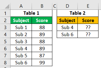
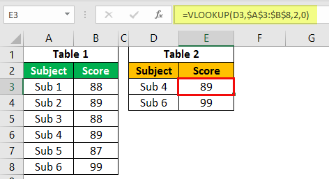
In table 1, we have the subject list and their respective scores, and in table 2, we have some subject names, but we do not have scores for them. So, using these subject names in table 2, we need to fetch the data from table 1.
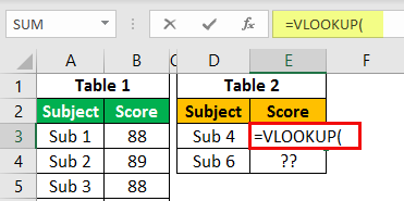
- First, let us open the VLOOKUP function in the E2 cell.
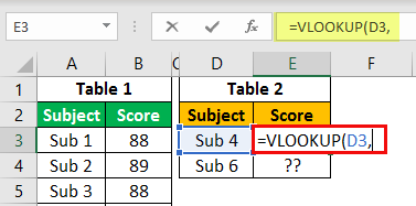
Then, select the LOOKUP value as a D3 cell.
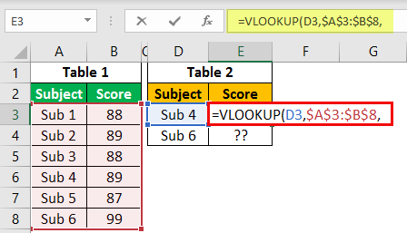
Next, we must select the table array as A3 to B8 and press the F4 key to make them an absolute reference.
Column Index Number is from the selected table array from which column you need to fetch the data. So, in this case, from the second column, we need to bring the data.
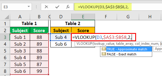
For the last argument range, LOOKUP, we must select FALSE as the option, or else we can enter.

Close the bracket and press the Enter key to get the score of Sub 4. Also, copy the formula and paste it to the below cell.
You have learned a formula to fetch values from different tables based on a LOOKUP value.
#2 IF Condition to Do Logical Test
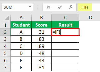
The Excel IF condition can be your friend in many situations because of its ability to conduct logical tests. For example, assume you want to test the scores of students and give the result. Below is the data for your reference.

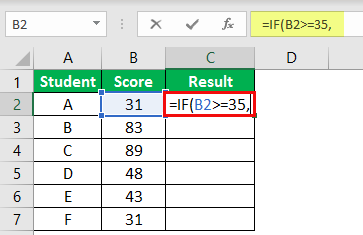
In the above table, we have students’ scores from the examination. So we need to arrive at the result as either “PASS” or “FAIL” based on these scores. So to reach these results criteria, if the score is >=35, the result should be “PASS” or else “FAIL.”
- We must first open the IF condition in the C2 cell.
- The first argument is logical to test.So, in this example, we need to do the logical test of whether the score is >=35, select the score cell B2, and apply the logical test as B2 >= 35.
- The next argument is value if true. If the applied logical test is “TRUE,” what is the value we need? If the logical test is “TRUE,” we need the result as “Pass.”
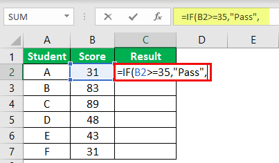
- So, the final part is value if false.If the applied logical test is “FALSE,” then we need the result as “Fail.”
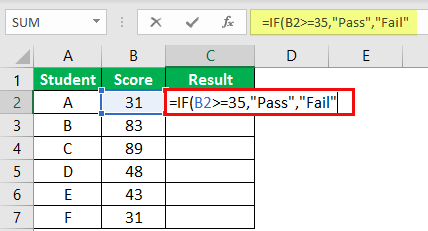
- Now, close the bracket, and we also need to fill the formula to the remaining cells.
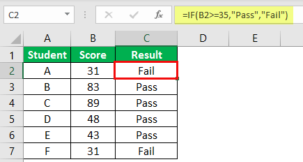
So, students A and F scored less than 35. Therefore, the result has arrived as “FAIL.”
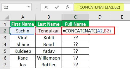
#3 CONCATENATE Function to Combine Two or More Values

- First, we need to open the CONCATENATE function in the C2 cell.
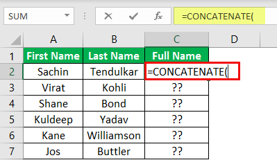
- For the first argument, “Text 1,“ select the “First Name” cell, and for “Text 2,” choose the “Last Name” cell.
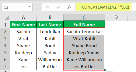
- Then, we need to apply the formula to all the cells to get the full name.

- If you want space as the “First Name” and “Last Name” separator, we can use the space character in double-quotes after selecting the first name.
#4 Count Only Numerical Values
If we want to count only numerical values from the range, you need to use the COUNT function in Excel. Take a look at the below data.
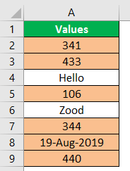
From the above table, we need to count only numerical values. For this, we can use the COUNT function.
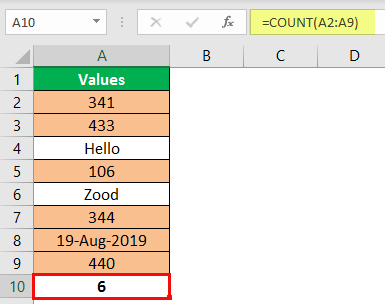
The result of the COUNT function is 6. The total count of cells is 8, but we have got the count of numerical values as 6. In cells A4 and A6, we have text values, but in cell A8, we have date values. The Excel COUNT function treats the date also as a numerical value only.
Note: “Date” and “Time” values are numerical values if the formatting is correct. Otherwise, they will be treated as “text” values.
#5 Count All Values

We got the count as 8 because the COUNTA function has counted all the cell values.
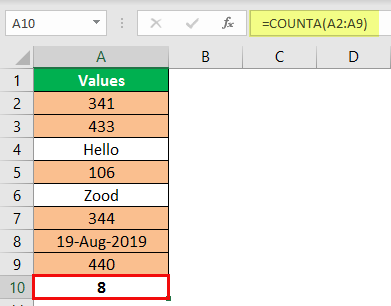
Note: Both the COUNT and COUNTA functions ignore blank cells.
#6 Count Based on Condition
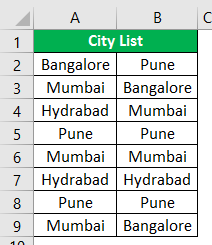
From this “City List,” if we want to count how many times “Bangalore” city is mentioned, we must open the COUNTIF function.

The first argument is “RANGE,” so we need to select the range of values from A2 to B9.
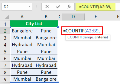
The second argument is “Criteria,” i.e., what you want to count, i.e., “Bangalore.
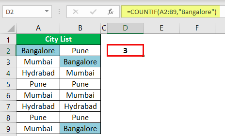
Bangalore has appeared three times in the range A2 to B9, so the COUNTIF function returns 3 as the count.
#7 Count Number of Characters in the Cell
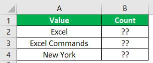
“Excel” has 5 characters, so the result is 5.
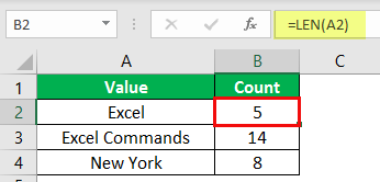
Note: Space is also considered as one character.
#8 Convert Negative Value to Positive Value
#9 Convert All Characters to UPPERCASE Values
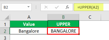
And if we want to convert all the text values to LOWERCASE values, then use the LOWER formula.
#10 Find Maximum and Minimum Values

Things to Remember
- These are some of the important formulas/commands in excel which are used regularly.
- We can also use these functions at the advanced level.
- There are more advanced formulas in Excel which come under advanced level courses.
- Space is considered one character.
Recommended Articles
This article is a guide to Excel Commands. Here, we discuss the top 10 commands in Excel, examples, and a downloadable template. You may learn more about Excel from the following articles: –
Источник
I’m trying to tell EXCEL that
IF G2<>I2, THEN use [ABS((H2-F2)/SQRT(((G2^2)/C2)+((I2^2)/D2)))] to fill AE,
BUT IF L2 is BLANK, leave AE empty. I’m trying the following with no success:
=IF(G2<>I2, ABS((H2-F2)/SQRT(((G2^2)/C2)+((I2^2)/D2))), L2, or(if(ISBLANK((l2))=true, "")))
asked Oct 3, 2016 at 4:11
If L2 is blank needs to be evaluated first because if it is blank then AE2 must be blank, regardless of the values of G2 and I2.
If L2 is not blank then go on to your secondary test.
=IF(ISBLANK(L2),"",IF(G2<>I2,ABS((H2-F2)/SQRT(((G2^2)/C2)+((I2^2)/D2)))))
answered Oct 3, 2016 at 4:41
![]()
Mark FitzgeraldMark Fitzgerald
3,0183 gold badges24 silver badges29 bronze badges
Элемент управления пользовательской формы CommandButton, используемый в VBA Excel для запуска процедур и макросов. Свойства кнопки, примеры кода с ней.
UserForm.CommandButton – это элемент управления пользовательской формы, предназначенный исключительно для запуска процедур и макросов VBA Excel.

Для запуска процедур и макросов обычно используется событие кнопки – Click.
Свойства элемента CommandButton
| Свойство | Описание |
|---|---|
| AutoSize | Автоподбор размера кнопки. True – размер автоматически подстраивается под длину введенной надписи (заголовка). False – размер элемента управления определяется свойствами Width и Height. |
| BackColor | Цвет элемента управления CommandButton. |
| Caption | Надпись (заголовок) – текст, отображаемый на кнопке. |
| ControlTipText | Текст всплывающей подсказки при наведении курсора на кнопку. |
| Enabled | Возможность взаимодействия пользователя с элементом управления CommandButton. True – взаимодействие включено, False – отключено (цвет надписи становится серым). |
| Font | Шрифт, начертание и размер текста надписи. |
| Height | Высота элемента управления. |
| Left | Расстояние от левого края внутренней границы пользовательской формы до левого края элемента управления. |
| Picture | Добавление изображения вместо текста заголовка или дополнительно к нему. |
| PicturePosition | Выравнивание изображения и текста на кнопке. |
| TabIndex | Определяет позицию элемента управления в очереди на получение фокуса при табуляции, вызываемой нажатием клавиш «Tab», «Enter». Отсчет начинается с 0. |
| Top | Расстояние от верхнего края внутренней границы пользовательской формы до верхнего края элемента управления. |
| Visible | Видимость элемента управления CommandButton. True – элемент отображается на пользовательской форме, False – скрыт. |
| Width | Ширина элемента управления. |
| WordWrap | Перенос текста заголовка на новую строку при достижении ее границы. True – перенос включен, False – перенос выключен. |
В таблице перечислены только основные, часто используемые свойства кнопки. Все доступные свойства отображены в окне Properties элемента управления CommandButton.

Пример кнопки с надписью и изображением
Примеры кода VBA Excel с кнопкой
Изначально для реализации примеров на пользовательскую форму UserForm1 добавлена кнопка CommandButton1.
Пример 1
Изменение цвета и надписи кнопки при наведении на нее курсора.
Условие примера 1
- Действия при загрузке формы: замена заголовка формы по умолчанию на «Пример 1», замена надписи кнопки по умолчанию на «Кнопка», запись цвета кнопки по умолчанию в переменную уровня модуля.
- Сделать, чтобы при наведении курсора на кнопку, она изменяла цвет на зеленый, а надпись «Кнопка» менялась на надпись «Нажми!»
- Добавление кода VBA Excel, который будет при удалении курсора с кнопки возвращать ей первоначальные настройки: цвет по умолчанию и надпись «Кнопка».
Решение примера 1
1. Объявляем в разделе Declarations модуля пользовательской формы (в самом начале модуля, до процедур) переменную myColor:
2. Загружаем пользовательскую форму с заданными параметрами:
|
Private Sub UserForm_Initialize() Me.Caption = «Пример 1» With CommandButton1 myColor = .BackColor .Caption = «Кнопка» End With End Sub |
3. Меняем цвет и надпись кнопки при наведении на нее курсора мыши:
|
Private Sub CommandButton1_MouseMove(ByVal _ Button As Integer, ByVal Shift As Integer, _ ByVal X As Single, ByVal Y As Single) With CommandButton1 .BackColor = vbGreen .Caption = «Нажми!» End With End Sub |
4. Возвращаем цвет и надпись кнопки при удалении с нее курсора мыши:
|
Private Sub UserForm_MouseMove(ByVal _ Button As Integer, ByVal Shift As Integer, _ ByVal X As Single, ByVal Y As Single) With CommandButton1 .BackColor = myColor .Caption = «Кнопка» End With End Sub |

Все процедуры размещаются в модуле пользовательской формы. Переменная myColor объявляется на уровне модуля, так как она используется в двух процедурах.
Пример 2
Запуск кода, размещенного внутри процедуры обработки события Click элемента управления CommandButton:
|
Private Sub CommandButton1_Click() MsgBox «Код внутри обработки события Click» End Sub |
Пример 3
Запуск внешней процедуры из процедуры обработки события Click элемента управления CommandButton.
Внешняя процедура, размещенная в стандартном модуле проекта VBA Excel:
|
Sub Test() MsgBox «Запуск внешней процедуры» End Sub |
Вызов внешней процедуры из кода обработки события Click
- с ключевым словом Call:
|
Private Sub CommandButton1_Click() Call Test End Sub |
- без ключевого слова Call:
|
Private Sub CommandButton1_Click() Test End Sub |
Строки вызова внешней процедуры с ключевым словом Call и без него – равнозначны. На ключевое слово Call можно ориентироваться как на подсказку, которая указывает на то, что эта строка вызывает внешнюю процедуру.
List of Top 10 Commands in Excel
Whether in engineering, medicine, chemistry, or any field, an Excel spreadsheet is the common tool for data maintenance. Some of them use it to maintain their database and others use this tool as a weapon to turn fortune for the respective companies they are working on. So, you, too, can turn things around for yourself by learning some of the most useful Excel commands.
Table of contents
- List of Top 10 Commands in Excel
- #1 VLOOKUP Function to Fetch Data
- #2 IF Condition to Do Logical Test
- #3 CONCATENATE Function to Combine Two or More Values
- #4 Count Only Numerical Values
- #5 Count All Values
- #6 Count Based on Condition
- #7 Count Number of Characters in the Cell
- #8 Convert Negative Value to Positive Value
- #9 Convert All Characters to UPPERCASE Values
- #10 Find Maximum and Minimum Values
- Things to Remember
- Recommended Articles
You can download this Commands in Excel Template here – Commands in Excel Template
#1 VLOOKUP Function to Fetch Data
The data in multiple sheets are common in many offices, but fetching the data from one worksheet to another and from one workbook to another is a challenge for beginners in Excel.
If you have struggled to fetch the data, VLOOKUPThe VLOOKUP excel function searches for a particular value and returns a corresponding match based on a unique identifier. A unique identifier is uniquely associated with all the records of the database. For instance, employee ID, student roll number, customer contact number, seller email address, etc., are unique identifiers.
read more will help you bring the data. For example, assume you have two tables below.
In table 1, we have the subject list and their respective scores, and in table 2, we have some subject names, but we do not have scores for them. So, using these subject names in table 2, we need to fetch the data from table 1.
- First, let us open the VLOOKUP function in the E2 cell.

- Then, select the LOOKUP value as a D3 cell.

- Next, we must select the table array as A3 to B8 and press the F4 key to make them an absolute reference.

- Column Index Number is from the selected table array from which column you need to fetch the data. So, in this case, from the second column, we need to bring the data.

- For the last argument range, LOOKUP, we must select FALSE as the option, or else we can enter.

- Close the bracket and press the Enter key to get the score of Sub 4. Also, copy the formula and paste it to the below cell.

You have learned a formula to fetch values from different tables based on a LOOKUP value.
#2 IF Condition to Do Logical Test
The Excel IF condition can be your friend in many situations because of its ability to conduct logical tests. For example, assume you want to test the scores of students and give the result. Below is the data for your reference.
In the above table, we have students’ scores from the examination. So we need to arrive at the result as either “PASS” or “FAIL” based on these scores. So to reach these results criteria, if the score is >=35, the result should be “PASS” or else “FAIL.”
- We must first open the IF condition in the C2 cell.
- The first argument is logical to test.So, in this example, we need to do the logical test of whether the score is >=35, select the score cell B2, and apply the logical test as B2 >= 35.
- The next argument is value if true. If the applied logical test is “TRUE,” what is the value we need? If the logical test is “TRUE,” we need the result as “Pass.”
- So, the final part is value if false.If the applied logical test is “FALSE,” then we need the result as “Fail.”
- Now, close the bracket, and we also need to fill the formula to the remaining cells.
So, students A and F scored less than 35. Therefore, the result has arrived as “FAIL.”
#3 CONCATENATE Function to Combine Two or More Values
If we want to combine two or more values from different cells, we can use the CONCATENATE function in excelThe CONCATENATE function in Excel helps the user concatenate or join two or more cell values which may be in the form of characters, strings or numbers.read more. For example, below is the “First Name” list and “Last Name.”
- First, we need to open the CONCATENATE function in the C2 cell.
- For the first argument, “Text 1,“ select the “First Name” cell, and for “Text 2,” choose the “Last Name” cell.
- Then, we need to apply the formula to all the cells to get the full name.
- If you want space as the “First Name” and “Last Name” separator, we can use the space character in double-quotes after selecting the first name.
#4 Count Only Numerical Values
If we want to count only numerical values from the range, you need to use the COUNT function in Excel. Take a look at the below data.
From the above table, we need to count only numerical values. For this, we can use the COUNT function.
The result of the COUNT function is 6. The total count of cells is 8, but we have got the count of numerical values as 6. In cells A4 and A6, we have text values, but in cell A8, we have date values. The Excel COUNT function treats the date also as a numerical value only.
Note: “Date” and “Time” values are numerical values if the formatting is correct. Otherwise, they will be treated as “text” values.
#5 Count All Values
If we want to count all the values in the range, we need to use the COUNTA functionThe COUNTA function is an inbuilt statistical excel function that counts the number of non-blank cells (not empty) in a cell range or the cell reference. For example, cells A1 and A3 contain values but, cell A2 is empty. The formula “=COUNTA(A1,A2,A3)” returns 2.
read more. We will apply the COUNTA function for the same data and see the count.
We got the count as 8 because the COUNTA function has counted all the cell values.
Note: Both the COUNT and COUNTA functions ignore blank cells.
#6 Count Based on Condition
If we want to count based on condition, we can use the COUNTIF functionThe COUNTIF function in Excel counts the number of cells within a range based on pre-defined criteria. It is used to count cells that include dates, numbers, or text. For example, COUNTIF(A1:A10,”Trump”) will count the number of cells within the range A1:A10 that contain the text “Trump”
read more. For example, look at the below data.
From this “City List,” if we want to count how many times “Bangalore” city is mentioned, we must open the COUNTIF function.
The first argument is “RANGE,” so we need to select the range of values from A2 to B9.
The second argument is “Criteria,” i.e., what you want to count, i.e., “Bangalore.
Bangalore has appeared three times in the range A2 to B9, so the COUNTIF function returns 3 as the count.
#7 Count Number of Characters in the Cell
If we want to count the number of characters in the cell, we need to use the LEN function in excelThe Len function returns the length of a given string. It calculates the number of characters in a given string as input. It is a text function in Excel as well as an inbuilt function that can be accessed by typing =LEN( and entering a string as input.read moreel. The LEN function returns the number of characters from the selected cell.
“Excel” has 5 characters, so the result is 5.
Note: Space is also considered as one character.
#8 Convert Negative Value to Positive Value
If we have negative values and want to convert them to positive ones, the ABS functionABS Excel function or Absolute function is used to calculate the absolute value of a given number. The negative numbers given as input are changed to positive numbers and if the argument provided to this function is positive, it remains unchanged.read more can do it for us.
#9 Convert All Characters to UPPERCASE Values
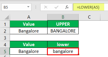
If we want to convert all the text values to UPPERCASE, we can use the UPPER formula in excelUppercase function in Excel is used to convert lowercase text to uppercase.read more.
And if we want to convert all the text values to LOWERCASE values, then use the LOWER formula.
#10 Find Maximum and Minimum Values
If we want to find maximum and minimum values, we may use MAX and MIN functions in excelIn Excel, the MIN function is categorized as a statistical function. It finds and returns the minimum value from a given set of data/array.read more, respectively.
Things to Remember
- These are some of the important formulas/commands in excel which are used regularly.
- We can also use these functions at the advanced level.
- There are more advanced formulas in Excel which come under advanced level courses.
- Space is considered one character.
Recommended Articles
This article is a guide to Excel Commands. Here, we discuss the top 10 commands in Excel, examples, and a downloadable template. You may learn more about Excel from the following articles: –
- Break-Even Point in Excel
- Basic Excel Formulas List
- Create Custom Functions in Excel
- Write Formula in Excel
Below is a brief overview of about 100 important Excel functions you should know, with links to detailed examples. We also have a large list of example formulas, a more complete list of Excel functions, and video training. If you are new to Excel formulas, see this introduction.
Note: Excel now includes Dynamic Array formulas, which offer important new functions.
Date and Time Functions
Excel provides many functions to work with dates and times.
NOW and TODAY
You can get the current date with the TODAY function and the current date and time with the NOW Function. Technically, the NOW function returns the current date and time, but you can format as time only, as seen below:

TODAY() // returns current date
NOW() // returns current time
Note: these are volatile functions and will recalculate with every worksheet change. If you want a static value, use date and time shortcuts.
DAY, MONTH, YEAR, and DATE
You can use the DAY, MONTH, and YEAR functions to disassemble any date into its raw components, and the DATE function to put things back together again.

=DAY("14-Nov-2018") // returns 14
=MONTH("14-Nov-2018") // returns 11
=YEAR("14-Nov-2018") // returns 2018
=DATE(2018,11,14) // returns 14-Nov-2018
HOUR, MINUTE, SECOND, and TIME
Excel provides a set of parallel functions for times. You can use the HOUR, MINUTE, and SECOND functions to extract pieces of a time, and you can assemble a TIME from individual components with the TIME function.

=HOUR("10:30") // returns 10
=MINUTE("10:30") // returns 30
=SECOND("10:30") // returns 0
=TIME(10,30,0) // returns 10:30
DATEDIF and YEARFRAC
You can use the DATEDIF function to get time between dates in years, months, or days. DATEDIF can also be configured to get total time in «normalized» denominations, i.e. «2 years and 6 months and 27 days».

Use YEARFRAC to get fractional years:

=YEARFRAC("14-Nov-2018","10-Jun-2021") // returns 2.57
EDATE and EOMONTH
A common task with dates is to shift a date forward (or backward) by a given number of months. You can use the EDATE and EOMONTH functions for this. EDATE moves by month and retains the day. EOMONTH works the same way, but always returns the last day of the month.

EDATE(date,6) // 6 months forward
EOMONTH(date,6) // 6 months forward (end of month)
WORKDAY and NETWORKDAYS
To figure out a date n working days in the future, you can use the WORKDAY function. To calculate the number of workdays between two dates, you can use NETWORKDAYS.

WORKDAY(start,n,holidays) // date n workdays in future
Video: How to calculate due dates with WORKDAY

NETWORKDAYS(start,end,holidays) // number of workdays between dates
Note: Both functions automatically skip weekends (Saturday and Sunday) and will also skip holidays, if provided. If you need more flexibility on what days are considered weekends, see the WORKDAY.INTL function and NETWORKDAYS.INTL function.
WEEKDAY and WEEKNUM
To figure out the day of week from a date, Excel provides the WEEKDAY function. WEEKDAY returns a number between 1-7 that indicates Sunday, Monday, Tuesday, etc. Use the WEEKNUM function to get the week number in a given year.

=WEEKDAY(date) // returns a number 1-7
=WEEKNUM(date) // returns week number in year
Engineering
CONVERT
Most Engineering functions are pretty technical…you’ll find a lot of functions for complex numbers in this section. However, the CONVERT function is quite useful for everyday unit conversions. You can use CONVERT to change units for distance, weight, temperature, and much more.

=CONVERT(72,"F","C") // returns 22.2
Information Functions
ISBLANK, ISERROR, ISNUMBER, and ISFORMULA
Excel provides many functions for checking the value in a cell, including ISNUMBER, ISTEXT, ISLOGICAL, ISBLANK, ISERROR, and ISFORMULA These functions are sometimes called the «IS» functions, and they all return TRUE or FALSE based on a cell’s contents.

Excel also has ISODD and ISEVEN functions that will test a number to see if it’s even or odd.
By the way, the green fill in the screenshot above is applied automatically with a conditional formatting formula.
Logical Functions
Excel’s logical functions are a key building block of many advanced formulas. Logical functions return the boolean values TRUE or FALSE. If you need a primer on logical formulas, this video goes through many examples.
AND, OR and NOT
The core of Excel’s logical functions are the AND function, the OR function, and the NOT function. In the screen below, each of these function is used to run a simple test on the values in column B:

=AND(B5>3,B5<9)
=OR(B5=3,B5=9)
=NOT(B5=2)
- Video: How to build logical formulas
- Guide: 50 examples of formula criteria
IFERROR and IFNA
The IFERROR function and IFNA function can be used as a simple way to trap and handle errors. In the screen below, VLOOKUP is used to retrieve cost from a menu item. Column F contains just a VLOOKUP function, with no error handling. Column G shows how to use IFNA with VLOOKUP to display a custom message when an unrecognized item is entered.

=VLOOKUP(E5,menu,2,0) // no error trapping
=IFNA(VLOOKUP(E5,menu,2,0),"Not found") // catch errors
Whereas IFNA only catches an #N/A error, the IFERROR function will catch any formula error.
IF and IFS functions
The IF function is one of the most used functions in Excel. In the screen below, IF checks test scores and assigns «pass» or «fail»:

Multiple IF functions can be nested together to perform more complex logical tests.
New in Excel 2019 and Excel 365, the IFS function can run multiple logical tests without nesting IFs.

=IFS(C5<60,"F",C5<70,"D",C5<80,"C",C5<90,"B",C5>=90,"A")
Lookup and Reference Functions
VLOOKUP and HLOOKUP
Excel offers a number of functions to lookup and retrieve data. Most famous of all is VLOOKUP:

=VLOOKUP(C5,$F$5:$G$7,2,TRUE)
More: 23 things to know about VLOOKUP.
HLOOKUP works like VLOOKUP, but expects data arranged horizontally:

=HLOOKUP(C5,$G$4:$I$5,2,TRUE)
INDEX and MATCH
For more complicated lookups, INDEX and MATCH offers more flexibility and power:

=INDEX(C5:E12,MATCH(H4,B5:B12,0),MATCH(H5,C4:E4,0))
Both the INDEX function and the MATCH function are powerhouse functions that turn up in all kinds of formulas.
More: How to use INDEX and MATCH
LOOKUP
The LOOKUP function has default behaviors that make it useful when solving certain problems. LOOKUP assumes values are sorted in ascending order and always performs an approximate match. When LOOKUP can’t find a match, it will match the next smallest value. In the example below we are using LOOKUP to find the last entry in a column:

ROW and COLUMN
You can use the ROW function and COLUMN function to find row and column numbers on a worksheet. Notice both ROW and COLUMN return values for the current cell if no reference is supplied:

The row function also shows up often in advanced formulas that process data with relative row numbers.
ROWS and COLUMNS
The ROWS function and COLUMNS function provide a count of rows in a reference. In the screen below, we are counting rows and columns in an Excel Table named «Table1».

Note ROWS returns a count of data rows in a table, excluding the header row. By the way, here are 23 things to know about Excel Tables.
HYPERLINK
You can use the HYPERLINK function to construct a link with a formula. Note HYPERLINK lets you build both external links and internal links:

=HYPERLINK(C5,B5)
GETPIVOTDATA
The GETPIVOTDATA function is useful for retrieving information from existing pivot tables.

=GETPIVOTDATA("Sales",$B$4,"Region",I6,"Product",I7)
CHOOSE
The CHOOSE function is handy any time you need to make a choice based on a number:

=CHOOSE(2,"red","blue","green") // returns "blue"
Video: How to use the CHOOSE function
TRANSPOSE
The TRANSPOSE function gives you an easy way to transpose vertical data to horizontal, and vice versa.

{=TRANSPOSE(B4:C9)}
Note: TRANSPOSE is a formula and is, therefore, dynamic. If you just need to do a one-time transpose operation, use Paste Special instead.
OFFSET
The OFFSET function is useful for all kinds of dynamic ranges. From a starting location, it lets you specify row and column offsets, and also the final row and column size. The result is a range that can respond dynamically to changing conditions and inputs. You can feed this range to other functions, as in the screen below, where OFFSET builds a range that is fed to the SUM function:

=SUM(OFFSET(B4,1,I4,4,1)) // sum of Q3
INDIRECT
The INDIRECT function allows you to build references as text. This concept is a bit tricky to understand at first, but it can be useful in many situations. Below, we are using INDIRECT to get values from cell A1 in 5 different worksheets. Each reference is dynamic. If a sheet name changes, the reference will update.

=INDIRECT(B5&"!A1") // =Sheet1!A1
The INDIRECT function is also used to «lock» references so they won’t change, when rows or columns are added or deleted. For more details, see linked examples at the bottom of the INDIRECT function page.
Caution: both OFFSET and INDIRECT are volatile functions and can slow down large or complicated spreadsheets.
STATISTICAL Functions
COUNT and COUNTA
You can count numbers with the COUNT function and non-empty cells with COUNTA. You can count blank cells with COUNTBLANK, but in the screen below we are counting blank cells with COUNTIF, which is more generally useful.

=COUNT(B5:F5) // count numbers
=COUNTA(B5:F5) // count numbers and text
=COUNTIF(B5:F5,"") // count blanks
COUNTIF and COUNTIFS
For conditional counts, the COUNTIF function can apply one criteria. The COUNTIFS function can apply multiple criteria at the same time:

=COUNTIF(C5:C12,"red") // count red
=COUNTIF(F5:F12,">50") // count total > 50
=COUNTIFS(C5:C12,"red",D5:D12,"TX") // red and tx
=COUNTIFS(C5:C12,"blue",F5:F12,">50") // blue > 50
Video: How to use the COUNTIF function
SUM, SUMIF, SUMIFS
To sum everything, use the SUM function. To sum conditionally, use SUMIF or SUMIFS. Following the same pattern as the counting functions, the SUMIF function can apply only one criteria while the SUMIFS function can apply multiple criteria.

=SUM(F5:F12) // everything
=SUMIF(C5:C12,"red",F5:F12) // red only
=SUMIF(F5:F12,">50") // over 50
=SUMIFS(F5:F12,C5:C12,"red",D5:D12,"tx") // red & tx
=SUMIFS(F5:F12,C5:C12,"blue",F5:F12,">50") // blue & >50
Video: How to use the SUMIF function
AVERAGE, AVERAGEIF, and AVERAGEIFS
Following the same pattern, you can calculate an average with AVERAGE, AVERAGEIF, and AVERAGEIFS.

=AVERAGE(F5:F12) // all
=AVERAGEIF(C5:C12,"red",F5:F12) // red only
=AVERAGEIFS(F5:F12,C5:C12,"red",D5:D12,"tx") // red and tx
MIN, MAX, LARGE, SMALL
You can find largest and smallest values with MAX and MIN, and nth largest and smallest values with LARGE and SMALL. In the screen below, data is the named range C5:C13, used in all formulas.

=MAX(data) // largest
=MIN(data) // smallest
=LARGE(data,1) // 1st largest
=LARGE(data,2) // 2nd largest
=LARGE(data,3) // 3rd largest
=SMALL(data,1) // 1st smallest
=SMALL(data,2) // 2nd smallest
=SMALL(data,3) // 3rd smallest
Video: How to find the nth smallest or largest value
MINIFS, MAXIFS
The MINIFS and MAXIFS. These functions let you find minimum and maximum values with conditions:

=MAXIFS(D5:D15,C5:C15,"female") // highest female
=MAXIFS(D5:D15,C5:C15,"male") // highest male
=MINIFS(D5:D15,C5:C15,"female") // lowest female
=MINIFS(D5:D15,C5:C15,"male") // lowest male
Note: MINIFS and MAXIFS are new in Excel via Office 365 and Excel 2019.
MODE
The MODE function returns the most commonly occurring number in a range:

=MODE(B5:G5) // returns 1
RANK
To rank values largest to smallest, or smallest to largest, use the RANK function:

Video: How to rank values with the RANK function
MATH Functions
ABS
To change negative values to positive use the ABS function.

=ABS(-134.50) // returns 134.50
RAND and RANDBETWEEN
Both the RAND function and RANDBETWEEN function can generate random numbers on the fly. RAND creates long decimal numbers between zero and 1. RANDBETWEEN generates random integers between two given numbers.

=RAND() // between zero and 1
=RANDBETWEEN(1,100) // between 1 and 100
ROUND, ROUNDUP, ROUNDDOWN, INT
To round values up or down, use the ROUND function. To force rounding up to a given number of digits, use ROUNDUP. To force rounding down, use ROUNDDOWN. To discard the decimal part of a number altogether, use the INT function.

=ROUND(11.777,1) // returns 11.8
=ROUNDUP(11.777) // returns 11.8
=ROUNDDOWN(11.777,1) // returns 11.7
=INT(11.777) // returns 11
MROUND, CEILING, FLOOR
To round values to the nearest multiple use the MROUND function. The FLOOR function and CEILING function also round to a given multiple. FLOOR forces rounding down, and CEILING forces rounding up.

=MROUND(13.85,.25) // returns 13.75
=CEILING(13.85,.25) // returns 14
=FLOOR(13.85,.25) // returns 13.75
MOD
The MOD function returns the remainder after division. This sounds boring and geeky, but MOD turns up in all kinds of formulas, especially formulas that need to do something «every nth time». In the screen below, you can see how MOD returns zero every third number when the divisor is 3:

SUMPRODUCT
The SUMPRODUCT function is a powerful and versatile tool when dealing with all kinds of data. You can use SUMPRODUCT to easily count and sum based on criteria, and you can use it in elegant ways that just don’t work with COUNTIFS and SUMIFS. In the screen below, we are using SUMPRODUCT to count and sum orders in March. See the SUMPRODUCT page for details and links to many examples.

=SUMPRODUCT(--(MONTH(B5:B12)=3)) // count March
=SUMPRODUCT(--(MONTH(B5:B12)=3),C5:C12) // sum March
SUBTOTAL
The SUBTOTAL function is an «aggregate function» that can perform a number of operations on a set of data. All told, SUBTOTAL can perform 11 operations, including SUM, AVERAGE, COUNT, MAX, MIN, etc. (see this page for the full list). The key feature of SUBTOTAL is that it will ignore rows that have been «filtered out» of an Excel Table, and, optionally, rows that have been manually hidden. In the screen below, SUBTOTAL is used to count and sum only the 7 visible rows in the table:

=SUBTOTAL(3,B5:B14) // returns 7
=SUBTOTAL(9,F5:F14) // returns 9.54
AGGREGATE
Like SUBTOTAL, the AGGREGATE function can also run a number of aggregate operations on a set of data and can optionally ignore hidden rows. The key differences are that AGGREGATE can run more operations (19 total) and can also ignore errors.
In the screen below, AGGREGATE is used to perform MIN, MAX, LARGE and SMALL operations while ignoring errors. Normally, the error in cell B9 would prevent these functions from returning a result. See this page for a full list of operations AGGREGATE can perform.

=AGGREGATE(4,6,values) // MAX ignore errors, returns 100
=AGGREGATE(5,6,values) // MIN ignore errors, returns 75
TEXT Functions
LEFT, RIGHT, MID
To extract characters from the left, right, or middle of text, use LEFT, RIGHT, and MID functions:

=LEFT("ABC-1234-RED",3) // returns "ABC"
=MID("ABC-1234-RED",5,4) // returns "1234"
=RIGHT("ABC-1234-RED",3) // returns "RED"
LEN
The LEN function will return the length of a text string. LEN shows up in a lot of formulas that count words or characters.

FIND, SEARCH
To look for specific text in a cell, use the FIND function or SEARCH function. These functions return the numeric position of matching text, but SEARCH allows wildcards and FIND is case-sensitive. Both functions will throw an error when text is not found, so wrap in the ISNUMBER function to return TRUE or FALSE (example here).

=FIND("Better the devil you know","devil") // returns 12
=SEARCH("This is not my beautiful wife","bea*") // returns 12
REPLACE, SUBSTITUTE
To replace text by position, use the REPLACE function. To replace text by matching, use the SUBSTITUTE function. In the first example, REPLACE removes the two asterisks (**) by replacing the first two characters with an empty string («»). In the second example, SUBSTITUTE removes all hash characters (#) by replacing «#» with «».

=REPLACE("**Red",1,2,"") // returns "Red"
=SUBSTITUTE("##Red##","#","") // returns "Red"
CODE, CHAR
To figure out the numeric code for a character, use the CODE function. To translate the numeric code back to a character, use the CHAR function. In the example below, CODE translates each character in column B to its corresponding code. In column F, CHAR translates the code back to a character.

=CODE("a") // returns 97
=CHAR(97) // returns "a"
Video: How to use the CODE and CHAR functions
TRIM, CLEAN
To get rid of extra space in text, use the TRIM function. To remove line breaks and other non-printing characters, use CLEAN.

=TRIM(A1) // remove extra space
=CLEAN(A1) // remove line breaks
Video: How to clean text with TRIM and CLEAN
CONCAT, TEXTJOIN, CONCATENATE
New in Excel via Office 365 are CONCAT and TEXTJOIN. The CONCAT function lets you concatenate (join) multiple values, including a range of values without a delimiter. The TEXTJOIN function does the same thing, but allows you to specify a delimiter and can also ignore empty values.

=TEXTJOIN(",",TRUE,B4:H4) // returns "red,blue,green,pink,black"
=CONCAT(B7:H7) // returns "8675309"
Excel also provides the CONCATENATE function, but it doesn’t offer special features. I wouldn’t bother with it and would instead concatenate directly with the ampersand (&) character in a formula.
EXACT
The EXACT function allows you to compare two text strings in a case-sensitive manner.

UPPER, LOWER, PROPER
To change the case of text, use the UPPER, LOWER, and PROPER function

=UPPER("Sue BROWN") // returns "SUE BROWN"
=LOWER("Sue BROWN") // returns "sue brown"
=PROPER("Sue BROWN") // returns "Sue Brown"
Video: How to change case with formulas
TEXT
Last but definitely not least is the TEXT function. The text function lets you apply number formatting to numbers (including dates, times, etc.) as text. This is especially useful when you need to embed a formatted number in a message, like «Sale ends on [date]».

=TEXT(B5,"$#,##0.00")
=TEXT(B6,"000000")
="Save "&TEXT(B7,"0%")
="Sale ends "&TEXT(B8,"mmm d")
More: Detailed examples of custom number formatting.
Dynamic Array functions
Dynamic arrays are new in Excel 365, and are a major upgrade to Excel’s formula engine. As part of the dynamic array update, Excel includes new functions which directly leverage dynamic arrays to solve problems that are traditionally hard to solve with conventional formulas. If you are using Excel 365, make sure you are aware of these new functions:
| Function | Purpose |
|---|---|
| FILTER | Filter data and return matching records |
| RANDARRAY | Generate array of random numbers |
| SEQUENCE | Generate array of sequential numbers |
| SORT | Sort range by column |
| SORTBY | Sort range by another range or array |
| UNIQUE | Extract unique values from a list or range |
| XLOOKUP | Modern replacement for VLOOKUP |
| XMATCH | Modern replacement for the MATCH function |
Video: New dynamic array functions in Excel (about 3 minutes).
Quick navigation
ABS, AGGREGATE, AND, AVERAGE, AVERAGEIF, AVERAGEIFS, CEILING, CHAR, CHOOSE, CLEAN, CODE, COLUMN, COLUMNS, CONCAT, CONCATENATE, CONVERT, COUNT, COUNTA, COUNTBLANK, COUNTIF, COUNTIFS, DATE, DATEDIF, DAY, EDATE, EOMONTH, EXACT, FIND, FLOOR, GETPIVOTDATA, HLOOKUP, HOUR, HYPERLINK, IF, IFERROR, IFNA, IFS, INDEX, INDIRECT, INT, ISBLANK, ISERROR, ISEVEN, ISFORMULA, ISLOGICAL, ISNUMBER, ISODD, ISTEXT, LARGE, LEFT, LEN, LOOKUP, LOWER, MATCH, MAX, MAXIFS, MID, MIN, MINIFS, MINUTE, MOD, MODE, MONTH, MROUND, NETWORKDAYS, NOT, NOW, OFFSET, OR, PROPER, RAND, RANDBETWEEN, RANK, REPLACE, RIGHT, ROUND, ROUNDDOWN, ROUNDUP, ROW, ROWS, SEARCH, SECOND, SMALL, SUBSTITUTE, SUBTOTAL, SUM, SUMIF, SUMIFS, SUMPRODUCT, TEXT, TEXTJOIN, TIME, TODAY, TRANSPOSE, TRIM, UPPER, VLOOKUP, WEEKDAY, WEEKNUM, WORKDAY, YEAR, YEARFRAC