
Хитрости »
30 Декабрь 2018 78571 просмотров
Невозможно разорвать связи с другой книгой
Прежде чем разобрать причины ошибки разрыва связей, не лишним будет разобраться что такое вообще связи в Excel и откуда они берутся. Если все это Вам известно — можете пропустить этот раздел 
- Что такое связи в Excel и как их создать
- Как разорвать/удалить связи
- Что делать, если связи не разрываются
Иногда при работе с различными отчетами приходится создавать связи с другими книгами(отчетами). Чаще всего это используется в функциях вроде ВПР(VLOOKUP) для получения данных по критерию из таблицы, расположенной в другой книге. Так же это может быть и простая ссылка на ячейки другой книги. В итоге ссылки в таких ячейках выглядят следующим образом:
=ВПР(A2;'[Продажи 2018.xlsx]Отчет’!$A:$F;4;0)
или
='[Продажи 2018.xlsx]Отчет’!$A1
- [Продажи 2018.xlsx] — обозначает книгу, в которой итоговое значение. Такие книги так же называют источниками
- Отчет — имя листа в этой книге
- $A:$F и $A1 — непосредственно ячейка или диапазон со значениями
Если закрыть книгу, на которую была создана такая ссылка, то ссылка сразу изменяется и принимает более «длинный» вид:
=ВПР(A2;’C:UsersДмитрийDesktop[Продажи 2018.xlsx]Отчет’!$A:$F;4;0)
=’C:UsersДмитрийDesktop[Продажи 2018.xlsx]Отчет’!$A1
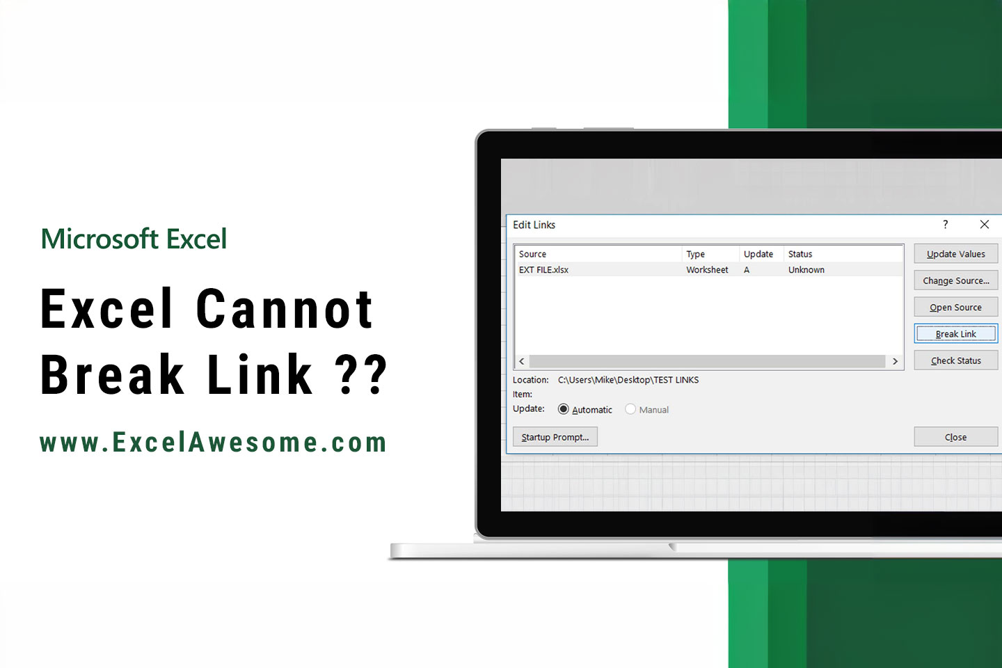
Предположу, что большинство такими ссылками не удивишь. Такие ссылки так же принято называть связыванием книг. Поэтому как только создается такая ссылка на вкладке Данные(Data) в группе Запросы и подключения(Queries & Coonections) активируется кнопка Изменить связи(Edit Links). Там же, как несложно догадаться, их можно изменить. В большинстве случаев ни использование связей, ни их изменение не доставляет особых проблем. Даже если в книге источники были изменены значения ячеек, то при открытии книги со связью эти изменения будут так же автоматом обновлены. Но если книгу-источник переместили или переименовали — при следующем открытии книги со ссылками на неё Excel покажет сообщение о недоступных связях в книге и запрос на обновление этих ссылок:

Если нажать Продолжить, то ссылки обновлены не будут и в ячейках будут оставлены значения на момент последнего сохранения. Происходит это потому, что ссылки хранятся внутри самой книги и так же там хранятся значения этих ссылок. Если же нажать Изменить связи(Change Source), то появится окно изменения связей, где можно будет выбрать каждую связь и указать правильное расположение нужного файла:

Так же изменение связей доступно непосредственно из вкладки Данные(Data)
Как разорвать связи
Как правило связи редко нужны на продолжительное время, т.к. они неизбежно увеличивают размер файла, особенно, если связей много. Поэтому чаще всего связь создается только для единовременно получения данных из другой книги. Исключениями являются случаи, когда связи делаются на общий файл, который ежедневного изменяется и дополняется различными сотрудниками и подразделениями, а в итоговом файле необходимо использовать именно актуальные данные этого файла.
Если решили разорвать связь, необходимо перейти на вкладку
Данные(Data)
-группа
Запросы и подключения(Queries & Coonections)
—
Изменить связи(Edit Links)
:
Выделить нужные связи и нажать
Разорвать связь(Break Link)
. При этом все ячейки с формулами, содержащими связи, будут преобразованы в значения вычисленные этой формулой при последнем обновлении. Данное действие нельзя будет отменить — только закрытием книги без сохранения.
Так же связи внутри формул разрываются, если формулы просто заменить значениями -выделяем нужные ячейки -копируем их -не снимая выделения жмем
Правую кнопку мыши
—
Специальная вставка(Paste Special)
—
Значения(Values)
. Формулы в ячейках будут заменены результатами их вычислений, а все связи будут удалены.
Более подробно про замену формул значениями можно узнать из статьи: Как удалить в ячейке формулу, оставив значения?
Что делать, если связи не разрываются
Но иногда возникают ситуации, когда вроде все формулы во всех ячейках уже заменены на значения, но запрос на обновление каких-то связей все равно появляется. В этом случае есть парочка рекомендаций для поиска и удаления этих мифических связей:
- проверьте нет ли каких-либо связей в именованных диапазонах:
нажмите сочетание клавиш Ctrl+F3 или перейдите на вкладку Формулы(Formulas) —Диспетчер имен(Name Manager)
Читать подробнее про именованные диапазоны
Если в каком-либо имени есть ссылка с полным путем к какой-то книге(вроде такого ‘[Продажи 2018.xlsx]Отчет’!$A1), то такое имя надо либо изменить, либо удалить. Кстати, некоторые имена в итоге могут выдавать ошибку #ССЫЛКА!(#REF!) — к ним тоже стоит присмотреться. Имена с ошибками ничего хорошего как правило не делают.
Настоятельно рекомендую перед удалением имен создать резервную копию файла, т.к. неверное удаление таких имен может повлечь неправильную работу файла даже в случае, если сами ссылки возвращали в итоге ошибочное значение. - если удаление лишних имен не дает эффекта — проверьте условное форматирование:
вкладка Главная(Home) —Условное форматирование(Conditional formatting) —Управление правилами(Manage Rules). В выпадающем списке проверить каждый лист и условия в нем:

Может случиться так, что условие было создано с использованием ссылки на другие книги. Как правило Excel запрещает это делать, но если ссылка будет внутри какого-то именованного диапазона — то диапазон такой можно будет применить в УФ, но после его удаления в самом УФ это имя все равно остается и генерирует ссылку на файл-источник. Такие условия можно удалять без сомнений — они все равно уже не выполняются как положено и лишь создают «пустую» связь. - Так же не помешает проверить наличие лишних ссылок и среди проверки данных(Что такое проверка данных). Как правило связи могут быть в проверке данных с типом Список. Но как их отыскать, если проверка данных распространена на множество ячеек?
Находим все ячейки с проверкой данных: выделяем одну любую ячейку на листе -вкладка Главная(Home) -группа Редактирование(Editing) —Найти и выделить(Find & Select) —Выделить группу ячеек(Go to Special). Отмечаем Проверка данных(Data validation) —Всех(All). Жмем Ок. После этого можно выделить все эти ячейки каким-либо цветом, чтобы удобнее было потом просматривать. Но такой метод выделит ВСЕ ячейки с проверками данных, а не только ошибочные.
Конечно, если вариантов кроме как найти руками нет и ячеек немного – просто заходим в проверку данных каждой ячейки(выделяем эту ячейку -вкладка Данные(Data) —Проверка данных(Data validation)) и смотрим, есть ли там проблемная формула со ссылками на другие книги.
Можно поступить более кардинально – после того как выделили все ячейки с проверкой данных идем на вкладку Данные(Data) —Проверка данных(Data validation) и для всех ячеек в поле Тип данных(Allow) выбираем Любое значение(Any value). Это удалит все формулы из проверки данных всех ячеек.
Но если ни удаление всех проверок данных, ни проверка каждой ячейки не подходит — я предлагаю коротенький код, который отыщет все такие ссылки быстрее и сэкономит время:Option Explicit '--------------------------------------------------------------------------------------- ' Author : The_Prist(Щербаков Дмитрий) ' Профессиональная разработка приложений для MS Office любой сложности ' Проведение тренингов по MS Excel ' https://www.excel-vba.ru ' info@excel-vba.ru ' WebMoney - R298726502453; Яндекс.Деньги - 41001332272872 ' Purpose: '--------------------------------------------------------------------------------------- Sub FindErrLink() 'надо посмотреть в Данные -Изменить связи ссылку на файл-иточник 'и записать сюда ключевые слова в нижнем регистре(часть имени файла) 'звездочка просто заменяет любое кол-во символов, чтобы не париться с точным названием Const sToFndLink$ = "*продажи 2018*" Dim rr As Range, rc As Range, rres As Range, s$ 'определяем все ячейки с проверкой данных On Error Resume Next Set rr = ActiveSheet.UsedRange.SpecialCells(xlCellTypeAllValidation) If rr Is Nothing Then MsgBox "На активном листе нет ячеек с проверкой данных", vbInformation, "www.excel-vba.ru" Exit Sub End If On Error GoTo 0 'проверяем каждую ячейку на предмет наличия связей For Each rc In rr 'на всякий случай пропускаем ошибки - такое тоже может быть 'но наши связи должны быть без них и они точно отыщутся s = "" On Error Resume Next s = rc.Validation.Formula1 On Error GoTo 0 'нашли - собираем все в отдельный диапазон If LCase(s) Like sToFndLink Then If rres Is Nothing Then Set rres = rc Else Set rres = Union(rc, rres) End If End If Next 'если связь есть - выделяем все ячейки с такими проверками данных If Not rres Is Nothing Then rres.Select ' rres.Interior.Color = vbRed 'если надо выделить еще и цветом End If End Sub
Чтобы правильно использовать приведенный код, необходимо скопировать текст кода выше, перейти в редактор VBA(Alt+F11) -создать стандартный модуль(Insert —Module) и в него вставить скопированный текст. После чего вызвать макросы(Alt+F8 или вкладка Разработчик —Макросы), выбрать FindErrLink и нажать выполнить.
Есть пара нюансов:- Прежде чем искать ненужную связь необходимо определить её ссылку: Данные(Data) -группа Запросы и подключения(Queries & Coonections) —Изменить связи(Edit Links). Запомнить имя файла и записать в этой строке внутри кавычек:
Const sToFndLink$ = «*продажи 2018*»
Имя файла можно записать не полностью, все пробелы и другие символы можно заменить звездочкой дабы не ошибиться. Текст внутри кавычек должен быть в нижнем регистре. Например, на картинках выше есть связь с файлом «Продажи 2018.xlsx», но я внутри кода записал «*продажи 2018*» — будет найдена любая связь, в имени которой есть «продажи 2018». - Код ищет проверки данных только на активном листе
- Код только выделяет все найденные ячейки(обычное выделение), он ничего сам не удаляет
- Если надо подсветить ячейки цветом — достаточно убрать апостроф(‘) перед строкой
rres.Interior.Color = vbRed ‘если надо выделить еще и цветом
- Прежде чем искать ненужную связь необходимо определить её ссылку: Данные(Data) -группа Запросы и подключения(Queries & Coonections) —Изменить связи(Edit Links). Запомнить имя файла и записать в этой строке внутри кавычек:

Как правило после описанных выше действий лишних связей остаться не должно. Но если вдруг связи остались и найти Вы их никак не можете или по каким-то причинам разорвать связи не получается(например, лист со связью защищен)- можно пойти совершенно иным путем. Действует этот рецепт только для файлов новых форматов Excel 2007 и выше (если проблема с файлом более старого формата — можно пересохранить в новый формат):
- Обязательно делаем резервную копию файла, связи в котором никак не хотят разрываться
- Открываем файл при помощи любого архиватора(WinRAR отлично справляется, но это может быть и другой, работающий с форматом ZIP)
- В архиве перейти в папку xl -> externalLinks
- Сколько связей содержится в файле, столько файлов вида externalLink1.xml и будет внутри. Файлы просто пронумерованы и никаких сведений о том, к какому конкретному файлу относится эта связь на поверхности нет. Чтобы узнать какой файл .xml к какой связи относится надо зайти в папку «_rels» и открыть там каждый из имеющихся файлов вида externalLink1.xml.rels. Там и будет содержаться имя файла-источника.
- Если надо удалить только связь на конкретный файл — удаляем только те externalLink1.xml.rels и externalLink1.xml, которые относятся к нему. Если удалить надо все связи — удаляем все содержимое папки externalLinks
- Закрываем архив
- Открываем файл в Excel. Появится сообщение об ошибке вроде «Ошибка в части содержимого в Книге …». Соглашаемся. Появится еще одно окно с перечислением ошибочного содержимого. Нажимаем закрыть.
После этого связи должны быть удалены.
Если и это не помогло — скорее всего «битая» связь связана с ошибкой самого файла и лучшим решением будет перенести все данные в новый файл.
Так же см.:
Найти скрытые связи
Оптимизировать книгу
Статья помогла? Поделись ссылкой с друзьями!
![]() Видеоуроки
Видеоуроки
Поиск по меткам
Access
apple watch
Multex
Power Query и Power BI
VBA управление кодами
Бесплатные надстройки
Дата и время
Записки
ИП
Надстройки
Печать
Политика Конфиденциальности
Почта
Программы
Работа с приложениями
Разработка приложений
Росстат
Тренинги и вебинары
Финансовые
Форматирование
Функции Excel
акции MulTEx
ссылки
статистика
Trying to break Excel links but Excel can not break links? It may be because you have referred external file in the data source of Excel objects or validations. Excel warning messages become a headache if Excel cannot break links when tried.
In normal cases, it is easy to break links in Excel files by just Alt + A + K or by going to the Data tab-> Queries & Connection manually. Then you have to select the wanted link to break and press the “Break Link” button. This option allows you to break visible known normal external links.
But What if excel won’t break external links even after trying this method?
In this article, we will see methods to fix Excel links issue in the following cases,
Why excel can not break links?
Excel fails to break external links if they are used for Data Validation or defining names in Names Manager.
In normal cases, if external links are placed in Excel date cells you can select and see them, so you can delete, break or edit them manually. But if they are used in the following Excel features,
- Data Validations
- Defined Name range in Name Manage
- Charts
Excel won’t break them using the Edit link option, you have to break them manually. Hence, if links are from the missing files every time you open an Excel file following error message will keep appearing.

Here is how to break links in Excel
To break links you have to look for links used in the formula or data source of Excel features. If you found one, verify is it the same which causing the problem, and if “yes” then fix it.
1
Break Excel Links used in Data Validation
If external links are used in Data Validation or in Names Manager they are not available to access through applied data cells. It becomes more difficult when you don’t know exactly which cells of rows and columns are used in data validation.

Follow these steps,
Step-1: First identify & select the data range (i.e cells, columns, rows) that have applied data validation referring to external files. If you don’t know then simply select all (Ctrl + A)
Step-2: Then go to Data tab-> Data Validation (Alt + A + V+V).
If your selection is perfect then it will show you referring file address as shown in the above screenshot. Otherwise, it will not and you have to select a large cell range (i.e select all).
Step-3: Then click on “Clear All”. It will clear all data validations from selected cells and so links.
Note: Clear All will remove all applied data validation from the selected range. You have to again set up validation to the required cells.
2
Break Excel Links used in Name ranges
If external links are used in defining names in Names Manager you can delete or edit them by editing names only. You can not break these links from the Edit Links dialog.

Follow these steps,
Step-1: Goto Formula tab->Name Manager (Alt + M + N)
Step-2: Look for a defined name with an external link in the “Refers To” column
Step-3: Edit/Correct or delete the defined Name Range
Note: Deleting a defined Name will cause an error in cells that contain the same Name as part of the formula.
3
Break Excel Links used in Charts
Moving Excel charts to external files cause the creation of phantom links (links to external file you haven’t created). You have to look for a such link in the data source and code of Excel charts if there is any.

Follow these steps,
Step-1: Select Excel chart then Right click->Slect Data.. source
Step-2: Look for links with the external file name
Step-3: Edit/Correct or delete the defined source
If your links are in VBA code, select the item and press Alt + F11 to open the VBA project manager. here you can check if there is any external link that is causing the problem.
Some external links are hidden in the data source of data validation, names, and charts. You can remove hidden external links in Excel by looking inside sources of charts, names, and data validations.
Conclusion
Excel cannot break links if they are used in the data sources of Excel features and objects. Links may become ghost or phantom links if you move sheets, or objects (such as charts) to another sheet. It can also cause problems when you move, edit, or remove referred Excel files. You have to reconfigure and correct reference formulas and data sources to fix such link-related issues.
|
setner  Пользователь Сообщений: 31 |
|
|
Sanja Пользователь Сообщений: 14838 |
#2 25.07.2017 16:09:04
Что значит не работает? Вы нажимали на кнопку Break Links? Согласие есть продукт при полном непротивлении сторон. |
||
|
setner Пользователь Сообщений: 31 |
да. По ссылке есть скрин. Нажмаю, и никуда не пропадает этот линк |
|
Sanja Пользователь Сообщений: 14838 |
#4 25.07.2017 16:16:39 Попробуйте выполнить такой макрос. Автор gling
Согласие есть продукт при полном непротивлении сторон. |
||
|
setner Пользователь Сообщений: 31 |
Попробовал. Ничего не произошло. Связь все еще есть. Те 2 связи, которые удалялись break linkом, удалились с помощью макроса(т.е. все работает) Но 3 связь, которая не удаляется break linkом не удалилась и с помощью макроса |
|
Sanja Пользователь Сообщений: 14838 |
#6 25.07.2017 16:31:23 Еще метода, источник
Согласие есть продукт при полном непротивлении сторон. |
||
|
The_Prist  Пользователь Сообщений: 14181 Профессиональная разработка приложений для MS Office |
Нужен файл. Скорее всего сама связь закопана где-то в именах(Ctrl+F3). Посмотрите там. Может надо имя удалить с этой ссылкой. Даже самый простой вопрос можно превратить в огромную проблему. Достаточно не уметь формулировать вопросы… |
|
setner Пользователь Сообщений: 31 |
#8 25.07.2017 16:35:14
это как? о_О |
||
|
setner Пользователь Сообщений: 31 |
#9 25.07.2017 16:39:52
нет, там к сожалению нету |
||
|
The_Prist Пользователь Сообщений: 14181 Профессиональная разработка приложений для MS Office |
Без файла сложно сказать где закопана ссылка. Она может быть и в диаграммах, и в других объектах. Надо смотреть и искать. Даже самый простой вопрос можно превратить в огромную проблему. Достаточно не уметь формулировать вопросы… |
|
Sanja Пользователь Сообщений: 14838 |
#11 25.07.2017 16:43:39
Обыкновенно. Файл *.xlsx это по сути архив. Его можно открыть любым популярным архиватором Согласие есть продукт при полном непротивлении сторон. |
||
|
setner Пользователь Сообщений: 31 |
#12 25.07.2017 17:09:25 Получилось с удалением папки externalLinks. Способ немного варварский, но работает. Спасибо! |
Содержание
- [Fixed] Excel break links won’t break issue
- Why Excel can not break links?
- How to break links in excel?
- 1 Break Excel Links used in Data Validation
- 2 Break Excel Links used in Name ranges
- 3 Break Excel Links used in Charts
- Break link in excel not working, what to do ?
- How do I force break links in Excel?
- How do I remove hidden external links in Excel?
- How do I remove a ghost link in Excel?
- How do you fix external links in Excel?
- Conclusion
- Break link excel не работает
- Break a link to an external reference in Excel
- Break a link
- Delete the name of a defined link
- Need more help?
- Spreadsheet Tips and Tools for Finance Professionals
- 1. Unprotect Sheets in your Problem File
- 2. Attempt to Break Links
- 3. Delete Named Ranges to External Files
- 4. Delete Chart External Links
- Other Non-Chart Objects
- 4a. Delete any external links in Conditional Formats.
- 5. Save a copy of the problem file.
- 6. Change the file type to ‘xls’ then back to ‘xlsx’.
- 34 Comments on “Excel Cannot Break Link – The Ultimate Guide”
[Fixed] Excel break links won’t break issue
Trying to break excel links but excel can not break links? It may be because you have referred external file in the data source of excel objects or validations. Excel warning messages become a headache if excel cannot break links when tried.
In normal cases, it is easy to break links in excel files by just Alt + A + K or by going to Data tab-> Queries & Connection manually. Then you have to select the wanted link to break and press the “Break Link” button. This option allows you to break visible known normal external links.
But What if excel won’t break external links even after trying this method?
Why Excel can not break links?
Excel fails to break external links if they are used for Data Validation or defining names in Names Manager.
In normal cases, if external links are placed in excel date cells you can select and see them, so you can delete, break or edit them manually. But if they are used in the following excel features,
- Data Validations
- Defined Name range in Name Manage
- Charts
Excel won’t break them using the Edit link option, you have to break them manually. Hence, if links are from the missing files every time you open an excel file following error message will keep appearing.
How to break links in excel?
To break links you have to look for links used in the formula or data source of excel features. If you found one, verify is it the same which causing the problem, and if “yes” then fix it.
1 Break Excel Links used in Data Validation
If external links are used in Data Validation or in Names Manager they are not available to access through applied data cells. It becomes more difficult when you don’t know exactly which cells of rows and columns are used in data validation.
Follow these steps,
Step-1: First identify & select the data range (i.e cells, columns, rows) that have applied data validation referring to external files. If you don’t know then simply select all (Ctrl + A)
Step-2 : Then go to Data tab-> Data Validation (Alt + A + V+V).
If your selection is perfect then it will show you referring file address as shown in the above screenshot. Otherwise, it will not and you have to select a large cells range (i.e select all).
Step-3: Then click on “Clear All”. It will clear all data validations from selected cells and so links.
Note: Clear All will remove all applied data validation from the selected range. You have to again set up validation to the required cells.
2 Break Excel Links used in Name ranges
If external links are used in defining names in Names Manager you can delete or edit them by editing names only. You can not break these links from the Edit Links dialog.
Follow these steps,
Step-1: Goto Formula tab->Name Manager (Alt + M + N)
Step-2: Look for a defined name with an external link in the “Refers To” column
Step-3: Edit/Correct or delete defined Name range
Note: Deleting a defined Name will cause an error in cells that contain the same Name as part of the formula.
3 Break Excel Links used in Charts
Moving excel charts to external files cause the creation of phantom links (links to external file you haven’t create). You have to look for such link in data source and code of excel charts if there is any.
Follow these steps,
Step-1: Select excel chart then Right click->Slect Data.. source
Step-2: Look for links with the external file name
Step-3: Edit/Correct or delete defined source
If your links are in VBA code, select item and press Alt + F11 to open VBA project manager. here you can check if there is any external link that is causing the problem.
Break link in excel not working, what to do ?
If break link in excel is not working then you have to search and break links manually. Look for the links in data validation, name manager, and data source of charts. You can also use paid link break addon.
How do I force break links in Excel?
If excel cannot break links normally using the edit link option you can break it forcefully using the manual search and edit method. Look for phantom links in various excel features data sources. Such as data validation, charts, and name manager.
How do I remove hidden external links in Excel?
Some external links are hidden in the data source of data validation, names, and charts. You can remove hidden external links in excel by looking inside sources of charts, names, and data validations.
How do I remove a ghost link in Excel?
Ghost links also called phantom links, they are hidden in the data source and VBA code of excel object. You can remove ghost links by manually searching and editing. Check and verify data source of excel objects, formatted and validation applied cells.
How do you fix external links in Excel?
You can fix external links in excel by breaking them. If edit links (Alt+A+K) not working, look for external links in the data source of applied data validations, excel charts, and names manager. Also, look in the VBA code if applicable.
Conclusion
Excel cannot break links if they are used in the data sources of excel features and objects. Links may become a ghost or phantom links if you move sheets, objects (such as charts) to another sheet. It can also cause problems when you move, edit, or remove referred excel files. You have to reconfigure and correct reference formulas and data sources to fix such link-related issues.
Источник
Break link excel не работает
Break a link to an external reference in Excel
When you break a link to the source workbook of an external reference, all formulas that use the value in the source workbook are converted to their current values. For example, if you break the link to the external reference =SUM([Budget.xls]Annual!C10:C25), the SUM formula is replaced by the calculated value—whatever that may be. Also, because this action cannot be undone, you may want to save a version of the destination workbook as a backup.
If you use an external data range, a parameter in the query may be using data from another workbook. You may want to check for and remove any of these type of links.
Break a link
On the Data tab, in the Connections group, click Edit Links.

Note: The Edit Links command is unavailable if your file does not contain linked information.
In the Source list, click the link that you want to break.
To select multiple linked objects, hold down the CTRL key, and click each linked object.
To select all links, press Ctrl+A.
Click Break Link.
Delete the name of a defined link
If the link used a defined name, the name is not automatically removed. You may want to delete the name as well, by following these steps:
On the Formulas tab, in the Defined Names group, click Name Manager.
In the Name Manager dialog box, click the name that you want to change.
Click the name to select it.
Need more help?
You can always ask an expert in the Excel Tech Community or get support in the Answers community.
If you cannot break links in Excel® then follow these steps (backup your file first):
- Unprotect each sheet in your problem file: HOME RIBBON – (CELLS) FORMAT – PROTECT SHEETS
- Break links: DATA RIBBON – (CONNECTIONS) EDIT LINKS – Select sheet then BREAK LINK
- Delete all named ranges to external files: FORMULA RIBBON – (DEFINED NAMES) NAME MANAGER
- Check all chart series ranges: Right click chart – SELECT DATA – (SERIES) EDIT. Check each series, if any ranges are in external files then cut the range from the external file and paste in to problem file. Also check chart titles and data label ranges.
- Check Conditional Formats and Data Validation for similar phantom links.
- Save a copy of the problem file then:
- Rename it in file explorer: changing the extension from .xlsx to .zip.
- Navigate to the folder ‘FILENAME.zip>xl’ file and delete the folder named ‘externalLinks’.
- Rename the ZIP file from extension .zip to .xlsx
- Save the file as file type ‘xls’ then back to ‘xlsx’ (or whatever the original file type was). Create a backup before trying this.
Some of these problems can be fixed with our add-in: fix and speed up Excel® files tools FREE ADD-IN .
Lets go through each of those steps in more detail to make sure you can break links.
1. Unprotect Sheets in your Problem File
a) When the active sheet is protected and you try to edit links the BREAK LINK button will be grayed out. You will need to unprotect this sheet or go to another sheet before you try and break links.
b) If a cell within a protected sheet is linked to an external file then you won’t be able to break links. Excel® will give you a warning that the external link cannot be broken due to the sheet being protected.
Excel® won’t be helpful enough to tell you which sheet contains the external link so you may need to go searching for it. You can use our free audit tools to find all cells with external links .
If you are using Excel® 2010 or later you can go to FILE – INFO. Under PROTECT WORKBOOK at the top you will see a list of any protected sheets.
 Fig(a1)
Once all the sheet are unprotected you can go on the next step.
2. Attempt to Break Links
This step will succeed in breaking links unless there are “phantom links” with the workbook. We will come to these later.
The Break Link function replaces the external links in any formulas with constant values.
If you want to identify all cells with references to external workbooks before you carry out this process you can do so:
- Press CTRL+F
- Type “xl*]” in the ‘Find what:’ box (don’t include the inverted commas in the box)
- Select ‘Within:’ Workbook
- Select ‘Look in:’ Formulas
- Click ‘Find All’
You can now check the list of links before you proceed.
To break links click DATA RIBBON – (CONNECTIONS sub menu) EDIT LINKS
You will see a list of external links that your current file is linking to. You can click each of the files and then click BREAK LINK.
If BREAK LINK is grayed out then go back to step 1 as you must still have a protected sheet in your workbook.
Hopefully you have now broken links successfully. However, if you still cannot break the Excel® link then you need to proceed to the next step.
3. Delete Named Ranges to External Files
This is the most common type of phantom link. It is possible that named ranges used by a file are defined as a range of cells in an external workbook.
You can check these easily and delete any that refer to external files.
Click on FORMULA RIBBON – (DEFINED NAMES) NAME MANAGER
Select each named range that refers to an external workbook and click DELETE. If there are many named ranges then you may want to sort them by ‘Refers To’. This will group links to the same external file.
You can delete more than one named range at a time. Select one, hold shift then select the one at the end of the range you want to delete.
Note: you could use the free file fix and speed up tools to delete named ranges to external files . With the tool you can choose to omit open files when deleting links to external files.
Go back to check EDIT LINKS to see if this has resolved your phantom link problem. If you still cannot break link then go on the next step.
4. Delete Chart External Links
It is possible that some of the series data used by an Excel® chart has been moved to an external file. This will create a phantom link.
Check if your file has any charts. It is possible that your workbook has hidden sheets so you may need to unhide them and check these for charts as well.
If FILE-INFO is saying there are still hidden sheets then your file may have sheets that are ‘Very Hidden’. This is unlikely unless you or someone else has set the sheet ‘Visible’ property to xlVeryHidden in the Visual Basic Editor. Click FILE – CHECK FOR ISSUES – INSPECT DOCUMENT to find any hidden sheets. You can either click to remove the sheets. Or you can unhide them in the Visual Basic Editor (click ALT+F11). In the VBE you can click on the hidden sheet then change its visible property to xlVisible.
In each chart. Right click the chart then ‘SELECT DATA’. Click on each series then ‘EDIT’.
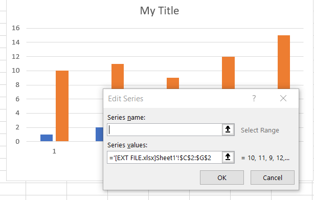
If you see a link to an external file in the name or values then you have found some phantom links. Go to this data in the external file, cut it and paste it in your problem workbook next to the chart.
 Fig(b1)
If you’ve already tried to BREAK LINKS to this file then instead of the file and range (above), all you will is a list of values (below).
 Fig(b3)
If this is the case then you’ll still need to cut the cells from the external file and paste in your problem workbook. The difficulty is going to be finding the cells. You don’t have a range reference in this case.
Also check the chart titles and other chart elements for external links such as this:
Other Non-Chart Objects
Other objects such as form controls or linked images may reference external files. You can check these as well before you go to the next step.
4a. Delete any external links in Conditional Formats.
UPDATE: Some links to external files can be hidden in any Excel feature that can reference sheet ranges. These features include Conditional Formats. (Thanks to Roger, Yuri and others in the comments for these additions)
Go through each sheet and select every cell. Click CTRL+A
For each of those rules: click on it then . You’ll need to check there are no references to external files in there. If there are then then amend or delete the rule. You can learn more about conditional formatting here if needed.
You can follow a similar process for Data Validation if you still have external links. To find data validation in a sheet you need to go to the menu then within the section click on then . Now select then click .
If you still cannot break links then try this:
5. Save a copy of the problem file.
This is the last resort if you cannot break links in Excel®. But this will resolve any remaining phantom link problems.
The downside is that this method is breaking external links without actually finding them. There is a chance this will impact the functionality of your workbook.
This method goes in to the file structure within the workbook to remove the link data.
- Create a copy of the file in which you are trying to remove the links
- In file explorer: right click this new file and RENAME
- Change the extension from .xlsx to .zip.
- Open this ZIP folder and navigate to the folder ‘FILENAME.zip > xl’
- Delete the folder named ‘externalLinks’.
- Back out of the ZIP folder
- Rename the ZIP folder from extension .zip back to .xlsx
- Open this file
When the file opens in Excel® you should not be asked to update links. The EDIT LINKS option should be grayed out.
Compare this new file with the original to ensure it is working correctly.
6. Change the file type to ‘xls’ then back to ‘xlsx’.
Update: this is added courtesy of the comment from Jack below. Thanks Jack.
This is the “last last” resort. Downgrade the file.
- Create a backup of your file.
- ‘Save As’ your workbook.
- Change the file type to ‘xls’ (Microsoft Excel 5.0/95 Workbook’
- Click ‘Save’
- ‘Save As’ again.
- Change the file type to ‘xlsx’
- Click ‘Save’
That may well fix any remaining problems.
There can be a downside to this method. Saving a file as ‘xls’ that was created as ‘xlsx’ may result in some features being removed from the file. You will receive a warning if there are any features that are incompatible with the ‘xls’ format so check that first. If there are any issues then your backup should bail you out.
Thank you so much!
I’d generated a bunch of filtered pivots from my main pivot and I kept getting a link error when I saved them separately. I can’t distribute them like that, and I couldn’t figure out where the connection was.
Followed your instructions, and clearing the named ranges worked like charm.
You sir are Awesome – thanks for posting this!
no. 5 is really awesome…
Thanks for all the tips.
However, I still had that “phantom” link.
Finally I saved the file with the downgraded extension from .xlsx to .xls.
Then with reopening the links had disappeared.
Maybe this can be helpful.
Thank you, Jack! It worked when nothing else posted here did!
I second this approach. All the above tricks work in most cases but for that extra sticky link, this is the only other approach, besides some possible VBA trick.
This is the only thing that fixed it, thanks!!
Thanks Jack. I included this tip in the post.
Cheers,
Mike
and one more issue – Conditional formatting, which can contain formulas linked to another workbook.
YES” This was my exact problem. It had been driving me up the wall. Thank you!
AMAZING!! Thank you so much for working this out!!
thanks the zip tip did the trick you are the Yoda of excel hacks
Thanks. I had tried all of your suggestions except for the ZIP file trick. That looked like it had real possibilities. But even that failed. I discovered the solution to my problem, which turned out to be a hidden link in a Data Validation rule. While the procedure described by user benalt at https://www.excelforum.com/excel-general/1024929-excel-file-wont-break-links.html did not exactly work, using the Find link in the Compatibility checker took me to the Data Validation cells that were problematic. I simply removed all the data validation on that worksheet and that solved my problem.
This is great. I knew to do everything but rename to zip file and delete external links folder. Thanks so much!
I had a link that would not break no matter what. I tried all the tips, even that suggested by the last commenter (Roger). None of this has worked to remove the link. Going back to historical versions, I was able to isolate it to two tabs in the file that had Data Validation.
In the end, I had to delete Data Validation in both tabs and then go to the end of the data in each tab, start with the first empty row after the data, highlight the next several using SHIFT+DOWN and then deleting those rows.
When I did that, the link magically disappeared forever!
So, somehow it was the combination of deleting all data validation and empty rows under the data that made the link disappear.
Through trial and error, I learned the link would not go away unless you FIRST removed the data validation in both tabs and then delete the empty rows of data each tab. The link did not disappear until I deleted the empty rows in the 2nd tab.
None of the above worked for me. It ended up being hidden in the data validation. Probably the same can happen with conditional formatting but that is easier to find. For validation you start by: Go To Special Data validation All. to see if any exist on that sheet. if it does you’ll have to check each cell by selecting it and selecting Data-> Data Validation and seeing rather the validation references an external cell. Many cells can also be selected and then Data->Data Validation it will let you know if one has different settings than the rest of the data validation which can be useful in finding the culprit.
Thank you yuri – everything failed for me – including (surprisingly) the zip file trick. Your comment about conditional formatting was correct – a couple of tabs had conditional formatting linking elsewhere……
click on [Home Tab], [Conditional Formatting], [Manage Rules], in the dropdown at the top [Show Formatting Rules For:] select each of your tabs in turn and look for anything that references an external sheet in either the rule or “applies to” columns.
Once I had done that and removed the external links, I was able to delete the link in the normal way from the [Data] tab and [Edit links] button.
Thank you. Best forum for solving this problem. I’ve been looking for a solution for months now.
Thanks very much! I had tried literally everything, including removing any problematic conditional formatting / data validation issues, but nothing worked… until I tried the renaming to .zip trick. No more annoying and inexplicable messages!
Jack – your suggestion was the right solution – non of the 5 points worked – but saving the file as .XLS worked – perfect.
For me, none of the article’s tips worked (however they do seem often useful!).
But thank you Jack, downgrading the file to .xls and back to .xlsx did the trick to me!
That is … just … awesome! OMG. Who knew that zipping a file exposed some of the guts of the file. I am forever humbled.
Massive thanks for that – I too was forced to use the rename-to-zip method (I’d heard of renaming files to zips, but never aware it was any use…). Got me out of a Deeep hole, so big thankyou!!
Thank you for this! I have been going batty over a link I couldn’t break. It never occured to me that it could be referenced in Conditional Formatting.
Awesome. You really helped me out here.
This is awesome. I had links to external workbooks in conditional formatting. All is fixed now.
I tried a few of these things – finally tried #6 – that worked…:-)
Источник
Use there quick fixes to get back to work in no time
by Matthew Adams
Matthew is a freelancer who has produced a variety of articles on various topics related to technology. His main focus is the Windows OS and all the things… read more
Updated on December 22, 2022
Reviewed by
Vlad Turiceanu

Passionate about technology, Windows, and everything that has a power button, he spent most of his time developing new skills and learning more about the tech world. Coming… read more
- Excel brings lots of functions that help us get our work done as fast as possible, but when the function we need doesn’t work it can be really annoying.
- Such a function can even be the Excel break links that if it’s not working can really be a pain.
- Fortunately, this article shows you exactly how to make it work again in a matter of minutes.

XINSTALL BY CLICKING THE DOWNLOAD FILE
This software will keep your drivers up and running, thus keeping you safe from common computer errors and hardware failure. Check all your drivers now in 3 easy steps:
- Download DriverFix (verified download file).
- Click Start Scan to find all problematic drivers.
- Click Update Drivers to get new versions and avoid system malfunctionings.
- DriverFix has been downloaded by 0 readers this month.
Some Excel users link their spreadsheets with reference links. A value in one Excel file will then be linked to another. Users can usually remove those reference links with the Edit Links dialog, which includes a Break Link option.
However, sometimes users encounter an error where the excel function to break links is not working. If you can’t break all reference links in an Excel file, check out some of the resolutions below.
How to fix the Excel function break links is not working?
- How to fix the Excel function break links is not working?
- 1. Unprotect the Excel worksheet
- 2. Delete named cell ranges
- 3. Clear all data validation rules from the sheet
- 4. Check out the Break Link Excel add-in
1. Unprotect the Excel worksheet
- Select Excel’s Review tab.
- Click the Unprotect Sheet button.

- If the sheet protection has a password, you’ll need to enter that password in the dialog window that opens.
- Click the OK button.
- Then the Break Link option might not be greyed out. Select the Data tab.
- Click the Edit Links option.

- Select the links listed, and click the Break Link option.


2. Delete named cell ranges
- Click the Formulas tab.
- Press the Name Manager button.

- Select a cell range name there.
- Press the Delete button to erase it.
- Click the OK option to confirm.
- Delete all the referenced cell range names listed within the Name Manager.
- Click the Close button.

3. Clear all data validation rules from the sheet
- Click the Select All button at the top left of a worksheet.

- Select the Data tab.
- Then click the Data Validation button.
- Select the Data Validation option.
- A dialog box should then open that asks to clear all.
- Press the OK button on that window.
- Repeat the above steps for other sheet tabs in the spreadsheet.

- Excel Running Slow? 4 Quick Ways to Make It Faster
- Fix: Excel Stock Data Type Not Showing
- Best Office Add-Ins: 15 Picks That Work Great in 2023
- Errors Were Detected While Saving [Excel Fix Guide]
4. Check out the Break Link Excel add-in
The Break Link Tool is an Excel add-in with which you can quickly remove all reference links from an Excel worksheet. The add-in is not freely available, but you can still try out the add-in with a one-week free trial.
Click the Download button on the Break Link Tool page to install that add-in.
With that add-in installed, you’ll see a Break Links button on the Home tab. Click that button to open the tool’s window. Then you can click a Select all option to select all the tool’s break link settings. Pressing the Start button will remove all the links.
So, that’s how you can break links in your sheet when you can’t get rid of them with the Edit Links tool. Note that spreadsheet objects and pivot tables might also include referral links.
So, also check if any objects and pivot tables on sheets have any reference links.
Which one of these methods worked out for you? Let us know by leaving a message in the comments section below.
Still having issues? Fix them with this tool:
SPONSORED
If the advices above haven’t solved your issue, your PC may experience deeper Windows problems. We recommend downloading this PC Repair tool (rated Great on TrustPilot.com) to easily address them. After installation, simply click the Start Scan button and then press on Repair All.
![]()