
Excel for Microsoft 365 Excel for Microsoft 365 for Mac Excel 2021 Excel 2021 for Mac Excel 2019 Excel 2019 for Mac Excel 2016 Excel 2016 for Mac Excel 2013 Excel 2010 Excel 2007 Excel for Mac 2011 More…Less
To add spacing between lines or paragraphs of text in a cell, use a keyboard shortcut to add a new line.
-
Double-click the cell in which you want to insert a line break
-
Click the location where you want to break the line.
-
Press ALT+ENTER to insert the line break.
Top of Page
Need more help?
Want more options?
Explore subscription benefits, browse training courses, learn how to secure your device, and more.
Communities help you ask and answer questions, give feedback, and hear from experts with rich knowledge.
A line break in Excel can be used to end the current line and start a new line in the same cell (as shown below).

Notice that in the pic above, Morning is in the second row in the same cell.
You may want to insert a line break in Excel when you have multiple parts of a text string that you want to show in separate lines. A good example of this could be when you have an address and you want to show each part of the address in a separate line (as shown below).

In this tutorial, I will show you a couple of ways to insert a line break in Excel (also called the in-cell carriage return in Excel)
Inserting a Line Break Using a Keyboard Shortcut
If you only need to add a couple of line breaks, you can do this manually by using a keyboard shortcut.
Here is how to insert a line break using a keyboard shortcut:
- Double-click on the cell in which you want to insert the line break (or press F2). This will get you into the edit mode in the cell
- Place the cursor where you want the line break.
- Use the keyboard shortcut – ALT + ENTER (hold the ALT key and then press Enter).
The above steps would insert a line break right where you had placed the cursor. Now you can continue to write in the cell and whatever you type will be placed in the next line.
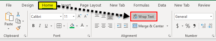
Note that you need the cell to be in the ‘Wrap text’ mode to see the content appear in the next line. In case it’s is not applied, you will see all the text in a single cell (even if you have the line break). ‘Wrap Text’ option is available in the Home tab in the ribbon.
The keyboard shortcut is a quick way to add a line break if you only have to do this for a few cells. But if you have to do this a lot of cells, you can use the other methods covered later in this tutorial.
Inserting Line Breaks Using Formulas
You can add a line break as a part of the formula result.
This can be useful when you have different cells that you want to combine and add a line break so that each part is in a different line.
Below is an example where I have used a formula to combined different parts of an address and have added a line break in each part.

Below is the formula that adds a line break within the formula result:
=A2&CHAR(10)&B2&(CHAR(10)&C2)
The above formula uses CHAR(10) to add the line break as a part of the result. CHAR(10) uses the ASCII code which returns a line feed. By placing the line feed where you want the line break, we are forcing the formula to break the line in the formula result.
You can also use the CONCAT formula instead of using the ampersand (&) symbol:
=CONCAT(A2,CHAR(10),B2,CHAR(10),C2)
or the old CONCATENATE formula in case you’re using older versions of Excel and don’t have CONCAT
=CONCATENATE(A2,CHAR(10),B2,CHAR(10),C2)
And in case you are using Excel 2016 or prior versions, you can use the below TEXTJOIN formula (which is a better way to join cells/ranges)
=TEXTJOIN(CHAR(10),TRUE,A2:C2)
Note that in order to get the line break visible in the cell, you need to make sure that ‘Wrap Text’ is enabled. If the Wrap Text is NOT applied, adding Char(10) would make no changes in the formula result.
Note: If you are using Mac, use Char(13) instead of Char(10).
Using Define Name Instead of Char(10)
If you need to use Char(10) or Char(13) often, a better way would be to assign a name to it by creating a defined name. This way, you can use a shortcode instead of typing the entire CHAR(10) in the formula.
Below are the steps to create a named range for CHAR(10)
Now you can use LB instead of =CHAR(10).
So the formula to combine address can now be:
=A2&LB&B2&LB&C2
Using Find and Replace (the CONTROL J Trick)
This is a super cool trick!
Suppose you have a dataset as shown below and you want to get a line break wherever there is a comma in the address.

If you want to insert a line break wherever there is a comma in the address, you can do that using the FIND and REPLACE dialog box.
Below are the steps to replace the comma with a line break:
- Select the cells in which you want to replace the comma with a line break
- Click the Home tab

- In the Editing group, click on Find and Select and then click on Replace (you can also use the keyboard shortcut Control + H). This will open the Find and Replace dialog box.

- In the Find and Replace dialog box, enter comma (,) in the Find What field.

- Place the cursor in the Replace Field and then use the keyboard shortcut – CONTROL + J (hold the Control key and then press J). This will insert the line feed in the field. You may be able to see a blinking dot in the field after you use Control + J
- Click on Replace ALL.
- Make sure Wrap text is enabled.


The above steps remove the comma and replace it with the line feed.
Note that if you use the keyboard shortcut Control J twice, this will insert the line feed (carriage return) two times and you will have a gap of two lines in between sentences.
You can also use the same steps if you want to remove all the line breaks and replace it will a comma (or any other character). Just reverse the ‘Find What’ and ‘Replace with’ entries.
You may also like the following Excel tutorials:
- Insert a watermark in Excel.
- Excel AUTOFIT: Make Rows/Columns Fit the Text Automatically
- Insert Picture in an Excel Cell.
- Add Bullet Points In Excel
- Insert a Check Mark Symbol in Excel
- 200+ Excel Keyboard Shortcuts.
- How to Create Named Ranges in Excel
You may need to split a value in your cell into two or more columns by space, character, or another delimiter. This can be done easily with a few clicks. On the other hand, some users need to split cells into rows. Although Excel does not have this functionality out of the box, you can use a few functions to do the job. Read on to learn all the options available for splitting cells in Excel.
You can split cells in Excel with the following options:
- Using a native functionality
- Using a combination of Excel functions
- Power Query
- Visual Basic for Applications (VBA)
For this article, we have decided to group the use cases not by option, but by the expected outcome. So, we’ll cover two epic tasks: split cells to columns and split cells to rows. Each of these tasks will include the options to split by different delimiters and other specific requirements.
For the examples below, we imported data from different sources such as Airtable, Google Sheets, and BigQuery with Coupler.io. It’s a powerful solution for getting data to Excel from multiple apps and web APIs without coding. The main benefit is that you can synchronize your workbook with your data source on a custom schedule!

Check out the Microsoft Excel integrations available.
Let’s check out each option so you can choose the one that works best for your task.
How to split one cell into two cells in Excel
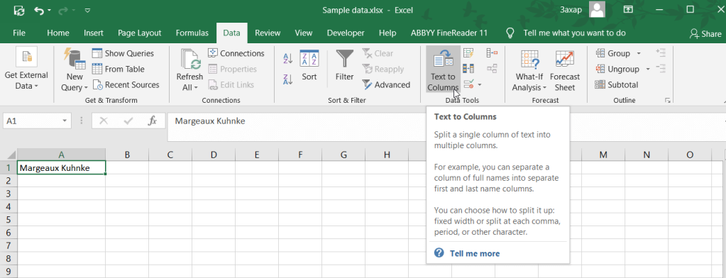
We’ll warm up with a simple example of splitting a full name, Margeaux Kuhnke, into first and last name cells. Go to the Data ribbon and click Text to Columns.
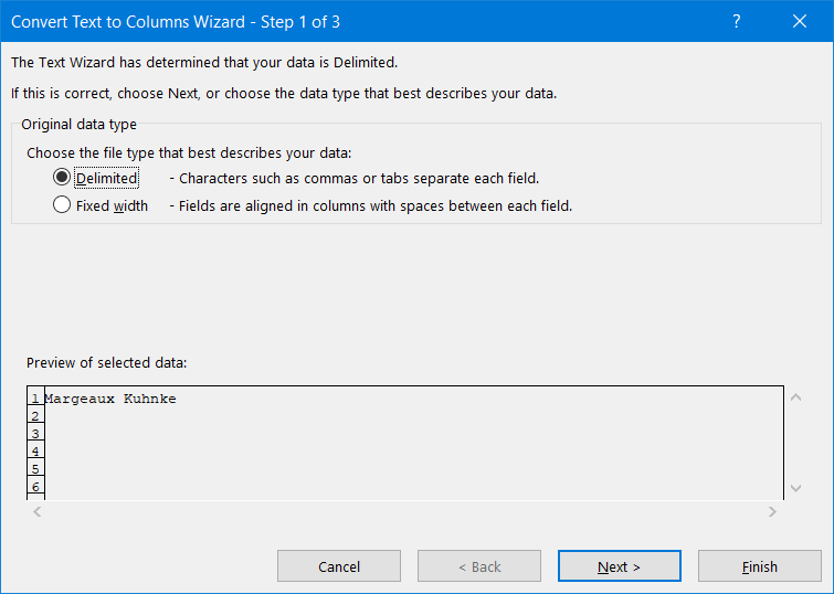
A wizard will open, where you’ll need to perform three steps:
- Choose the way to split your data: by a delimiter or by a fixed width
- Set delimiters or field width depending on which splitting method you chose before. In our example, we need to split a cell by space as a delimiter.

- Select the date format and destination cell. If you want to keep the source value, choose a different cell as a destination.

Once you click “Finish“, your cell will be split into the number of cells depending on the number of delimiters in your source value. In our example, we had one delimiter, so the cell was split into two cells.

Split text in Excel cell into multiple cells by space
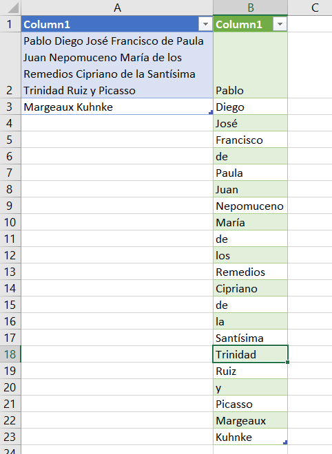
If a full name in a cell consists of three or more names, the number of split cells will be greater. For example, let’s split Pablo Picasso’s full name using space as a delimiter:
Pablo Diego José Francisco de Paula Juan Nepomuceno María de los Remedios Cipriano de la Santísima Trinidad Ruiz y Picasso

The outcome is that we’ve split the text in the Excel cell into multiple cells (20!) by spaces!

Excel split cells by character
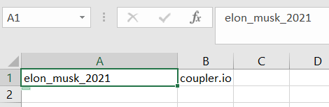
Splitting cells by character may be useful if you need to separate, for example, username and domain name in email addresses. Let’s say we have a fictional user with the following email address:
elon_musk_2021@coupler.io
In this case, the delimiter is a character: @. So, we need to specify this.

There you go!
Excel split data in cell by line break
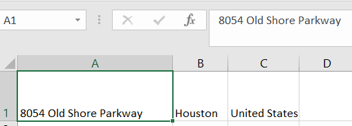
What if your cell contains a few lines like an address, and you want each line in its own cell?
8054 Old Shore Parkway
Houston
United States
To split this string, you need to specify the line break as a delimiter. To do this, choose Other as a delimiter and press Ctrl + J.

Here is the result:
How to split merged cells in Excel
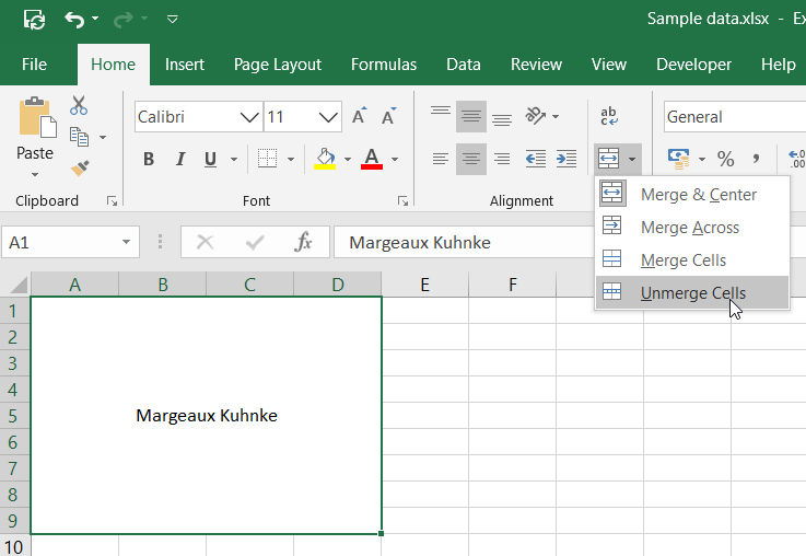
Splitting merged cells is a slightly different concept, since it does not affect the content of the cells. You can do this easily using the Merge & Center button.
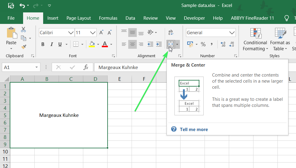
Select the merged cells, open the drop-down options and click Unmerge Cells.
Split cells into rows in Excel
Unfortunately, there is no single button or function to split a cell into rows or to split cells vertically in Excel. Nevertheless, you can do this with the help of Excel functions or Power Query. But first, check out this easy method for splitting cells into rows.
Split Excel cell into two rows easily
You’ll need to take two steps:
- Split your cell using the Text to Columns button as we explained before.

- Copy the resulting cells and paste them using Paste special => Transpose.

This is the simplest way to split cells to rows in Excel, but it’s manual. Let’s discover some options to automate the flow.
Split cells vertically in Excel with formulas
Let’s take the previous example of splitting a full name: Margeaux Kuhnke.
We’ll need two formulas for each row:
- First
= LEFT(cell, FIND(" ",cell) - 1)
This formula extracts a string before the specified delimiter: FIND(" ",cell).
2. Second
= RIGHT(cell, LEN(cell) - FIND(" ",cell))
This formula extracts a string after the specified delimiter.
If you have two or more delimiters, both formulas will only work with the first delimiter, like this:

If for some reason you need to split a cell by a second or third delimiter, you need to update the FIND formula, keeping the following logic in mind:
=FIND("delimiter",cell,starting_position)starting_position– specify the starting position (character) to skip the unnecessary delimiters.
In our example, to split the cell by the second delimiter, the formulas will look like this:
=LEFT(A1,FIND(" ",A1,10)-1)
=RIGHT(A1, LEN(A1) - FIND( " ",A1,10) )

Split cells in Excel into multiple rows
Unfortunately, these formulas do not apply to the “Pablo Picasso” case, where the number of delimiters is 19! For such cases, the following formula works better:
=FILTERXML("<t><s>" &SUBSTITUTE($cell," ", "</s><s>") & "</s></t>", "//s")This converts cell contents into an XML string and then extracts data from it. This formula should be executed as an array formula; that is, you need to select the cell to split into and press Ctrl+Shift+Enter. Here is how it works with the Pablo Picasso’s full name:
=FILTERXML("<t><s>" &SUBSTITUTE($A$1," ", "</s><s>") & "</s></t>", "//s")

You can also use this formula to extract specific pieces of your string by specifying them as follows:
=FILTERXML("<t><s>" &SUBSTITUTE($cell," ", "</s><s>") & "</s></t>", "//s"[number_of_piece])For example, to extract the third name from the Picasso’s full name, we update our formula as follows:
=FILTERXML("<t><s>" &SUBSTITUTE($A$1," ", "</s><s>") & "</s></t>", "//s[3]")

How to split cells to rows or columns in Excel dynamically without formulas
If you don’t want to mess with formulas for your splitting tasks, but you want to have a dynamic approach, check out the Power Query method. Let’s check it out for our Pablo Picasso example.
- Go to Data => From Table.
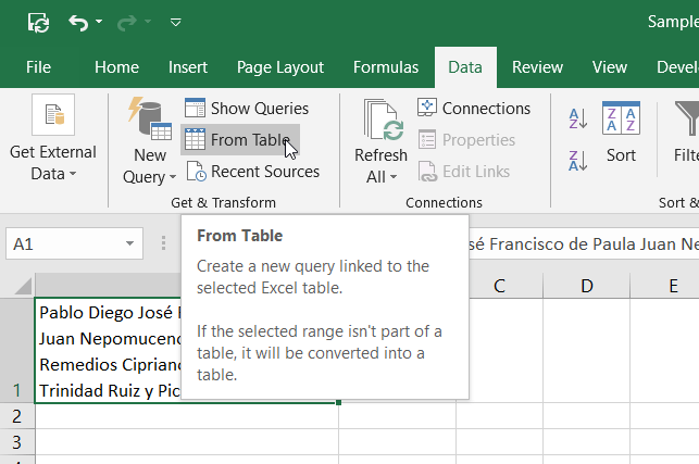
- Select the cell with your data and click “OK“.

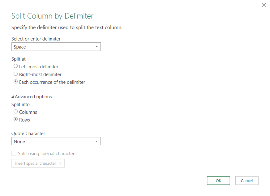
- After that, the Power Query Editor will open. Then select Split Column => By Delimiter.

- Select your delimiter, click “Advanced options“, choose Split into Rows, and select “None” as a Quote Character.
- The data will be split into rows. Now you need to save and load it. For this, click:
- “Close & Load” to load data in a new worksheet.
- “Close & Load To…” to specify a custom destination for your data.

There you go!

Now, every value added to the A column will be split into rows by space. Just click refresh to see the split values.
See, with Power Query you can also split cells into columns by different delimiters.
Bonus: How to split cells diagonally in Excel
By diagonal split, users usually mean crossing a cell with a diagonal border like this:
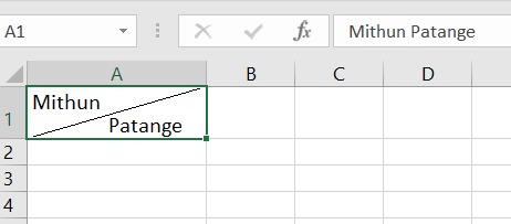
This does not split a cell into columns or rows, but makes a visual split of two values in the cell. Here is how you can do this.
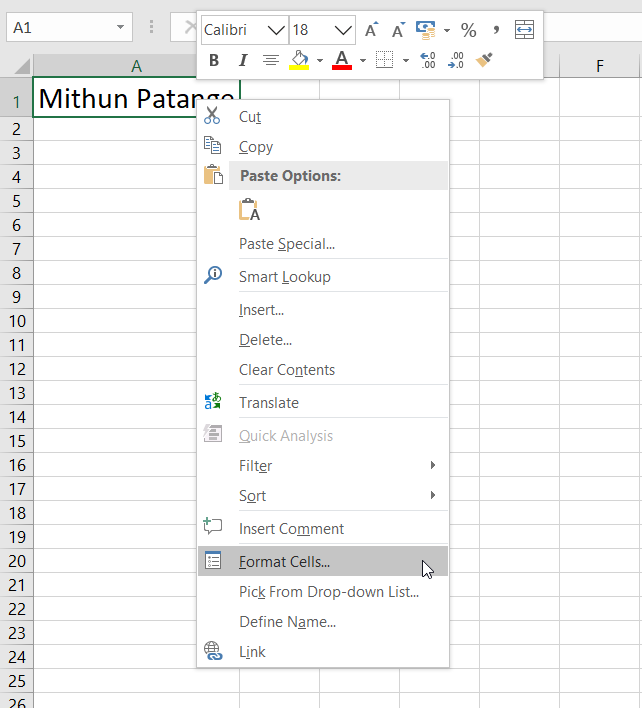
- Right-click on the cell you want to split diagonally and select Format Cells…
- In the open dialog window, go to the Border tab and click the diagonal border.
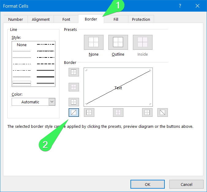
- Click OK and you will see a line splitting the selected cell diagonally. But this is not quite how we want it to look.

- To fix this, we need to assign the Superscript font effect to one value in the cell, and Subscript to the other value. Select one word – in our case, this is “Mithun“. Then go to the Home tab and click the Font Settings – a small arrow at the bottom-right corner of the Font section.
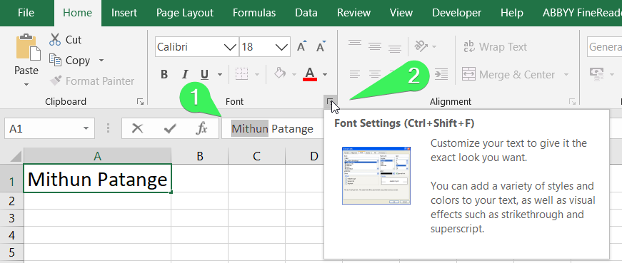
- In the dialog box, check the Superscript font effect and click OK.

- Here is how it looks now

- Now, do the same with the second value using the Subscript option.

- And there you go!
Are there other options to split cells in Excel?
In Excel, there is no dedicated function for splitting data, like SPLIT in Google Sheets. However, using Excel VBA, you can build a custom VBA function to solve your specific splitting tasks. This requires knowledge of Microsoft Visual Basic for Applications.
However, for most cases, the options previously described will do the job. Good luck with splitting your data!
-

A content manager at Coupler.io whose key responsibility is to ensure that the readers love our content on the blog. With 5 years of experience as a wordsmith in SaaS, I know how to make texts resonate with readers’ queries✍🏼

Back to Blog
Focus on your business
goals while we take care of your data!
Try Coupler.io
This post will guide you how to split cells with line break or carriage returns into multiple rows or columns in Excel. How do I split cell contents based on carriage returns into separate rows with Text to Columns in Excel. How to split Excel Cell with carriage returns into multiple rows using VBA Macro in Excel.
- Split Cell Contents with Carriage Returns into Multiple Rows using Text to Columns Feature
- Split Cell Contents with Carriage Returns into Multiple Rows using VBA Macro
- Video: Split Cell Contents with Carriage Returns into Multiple Rows
The Carriage returns also known as line breaks in Excel, and when you press “Alt+Enter” shortcut in a cell, one carriage returns will be generated. Or you copied the text string from other source, which already have the line breaks.
Table of Contents
- Split Cell Contents with Carriage Returns into Multiple Rows using Text to Columns Feature
- Split Cell Contents with Carriage Returns into Multiple Rows using VBA Macro
Split Cell Contents with Carriage Returns into Multiple Rows using Text to Columns Feature
Assuming that you have a list of data in range B1:B4, which contain text strings with carriage returns, and you want to split those cells based on the carriage returns or line breaks into separate rows or columns. How to achieve it. You can use the Text to Columns feature to achieve the result. just do the following steps:
#1 select the range of cells B1:B4 that you want to split.
#2 go to DATA tab, click Text to Columns command under Data Tools group. And the Text to Columns dialog box will open.
#3 choose the Delimited radio button under Original data type section. And click Next button.
#4 only check the Other check box in the Delimiters section, and select the text box of Other, and then press Ctrl + J shortcut in your keyboard. And you can see the expected result in the Data preview section. Click Next button.
#5 select one cell as the destination cell, such as: put the result in Cell C1, and you can type the value $C$1 in destination text box. and then click Finish button.
#6 let’s see the result:
Split Cell Contents with Carriage Returns into Multiple Rows using VBA Macro
You can also use an Excel VBA Macro to achieve the same result of splitting Cells with line breaks into multiple rows. Do the following steps:
#1 open your excel workbook and then click on “Visual Basic” command under DEVELOPER Tab, or just press “ALT+F11” shortcut.

#2 then the “Visual Basic Editor” window will appear.
#3 click “Insert” ->”Module” to create a new module.

#4 paste the below VBA code into the code window. Then clicking “Save” button.
Sub SplitCellsBaseLineBreak()
    Dim str() As String
    Dim myRng As Range
    Set myRng = Application.Selection
    Set myRng = Application.InputBox("select one range that you want to split", "SplitCellsBaseLineBreak", myRng.Address, Type:=8)

    For Each myCell In myRng
        If Len(myCell) Then
            str = VBA.Split(myCell, vbLf)
            myCell.Resize(1, UBound(str) + 1).Offset(0, 1) = str
        End If
    Next
End Sub
#5 back to the current worksheet, then run the above excel macro. Click Run button.
#6 select one range that you want to split, such as B1:B4, click Ok button.
#7 Let’s see the result.
Video: Split Cell Contents with Carriage Returns into Multiple Rows
What is a Line Break in Excel Cell?
Line break in Excel means inserting a new line in any cell value. Simply pressing the “Enter” key can take us to the next cell. We can use the keyboard shortcut, “ALT + Enter,” to insert a new line inside a cell to insert a line break. As we insert a line break, the cell’s height also increases as it represents the data in the cell.
Table of contents
- What is a Line Break in Excel Cell?
- How to Insert Line Break in Excel Cell?
- Method #1 – Line Break with Excel Formula (& Function)
- Method #2 – Line Break with Excel Formula (Concatenate)
- Method #3 – Line Break in Excel Cell (Conventional way)
- Things to Remember
- Recommended Articles
- How to Insert Line Break in Excel Cell?
How to Insert Line Break in Excel Cell?
- Concatenate Function in excelThe CONCATENATE function in Excel helps the user concatenate or join two or more cell values which may be in the form of characters, strings or numbers.read more.
- AND function
- Use of Alt + Enter Method.
You can download this Line Break Excel Template here – Line Break Excel Template
Method #1 – Line Break with Excel Formula (& Function)
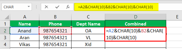
Suppose we have the name, phone number, and department name in a column. We want them in a single cell combined, but a line separates all three. The data is as follows:
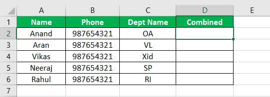
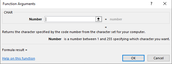
We want all the three data combined in one column D column and want each data to be separated by a line. We will learn the method of using the AND function in this example. But, first, we need to understand what a CHAR function is. Char function in excelThe character function in Excel, also known as the char function, identifies the character based on the number or integer accepted by the computer language. For example, the number for character «A» is 65, so if we use =char(65), we get A.read more: returns the character specified by our computer, a specific code.
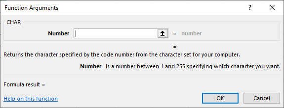
Char(10) returns a line break in the cell.
Below are the steps of inserting line break in Excel:
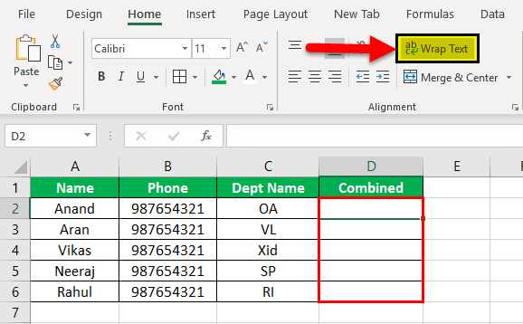
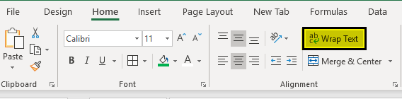
- Now, we need to wrap the text D column to see all the data in the D column.

- Select the blank cells opposite to the data in the D column.

- Click on the Excel Wrap Text in the Alignment section of the Home tab.

- Now in cell D2, we must write the following formula:

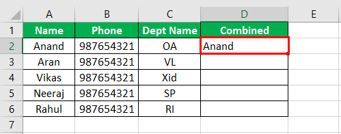
- Now, press the Enter key to see the result.

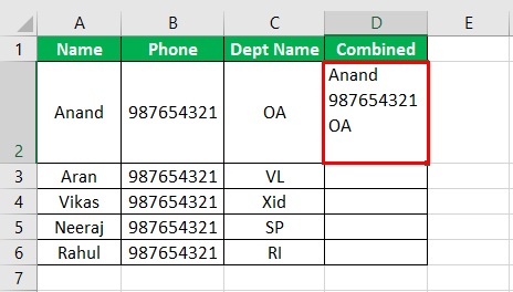
- We currently do not see the whole data; we need to expand the row by clicking on the expand row button by hovering our mouse between the two cells, A2 and A3.

- Now, drag the formula to cell D6.

We can see that we have successfully inserted a line break in cells using the AND formula.


Method #2 – Line Break with Excel Formula (Concatenate)
In the above example, we used the AND formula to insert a line break in a cell. We will learn to insert a line break in the cell using the CONCATENATE function. But first, what is a CONCATENATE function? The CONCATENATE function joins several strings or numbers, or values into a single string.
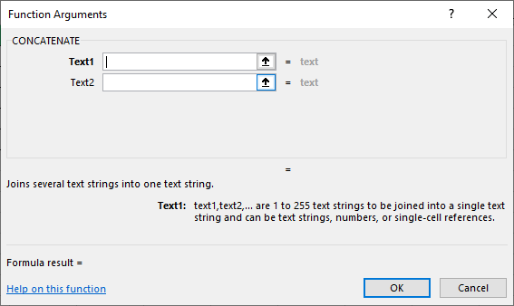
Also, we know what a CHAR function does, but for our revision, let us look again at what a char function does. The CHAR function returns the character specified by our computer, a specific code.
The CHAR(10) inserts a line break in a cell. Now, have a look at the below data:
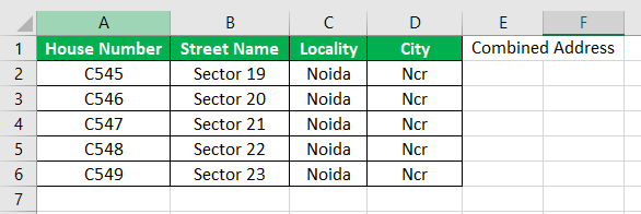
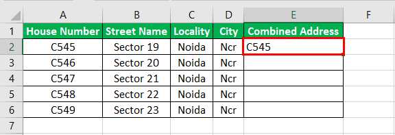
We have a house number, street name, locality, and city in columns A, B, C, and D. Like we fill out forms, it is the same. However, we want the combined address in the E column. We will use the CONCATENATE formula and the CHAR function to insert a line break in the cell.
- Step #1 – First, we need to wrap the text to see all the data.
- Step #2 – Select all the cells parallel to data in the E column.
- Step #3 – Now, click on “Wrap text” under the “Alignment” section in the “Home” tab.
- Step #4 – In cell E2, we must write the following formula:

- Step #5 – When we press the “Enter” key, we can see the following result:
- Step #6 – We currently do not see the whole data. We need to expand the row by clicking on the expand row button by hovering our mouse between the two cells, A2 and A3.
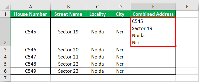
- Step #7 – Now, we must drag the formula to cell E8 and see the result.

We have successfully inserted a line break using the concatenate excel formulaThe CONCATENATE function in Excel helps the user concatenate or join two or more cell values which may be in the form of characters, strings or numbers.read more.
Method #3 – Line Break in Excel Cell (Conventional way)
We will use the last and the most convenient way of using a line break in a cell while working on data. We need to keep in mind that this method only works in a cell. For the next cell, we need to repeat the process. We cannot copy the same formula to other cells like a formula.
We will try to insert a line break in the sentence “I am a Boy” and insert a line break after every word.
- Step #1 – In any cell, double click on the cell or press the F2 button to get in the cell.
- Step #2 – Write I and press the “Alt + Enter” keys.
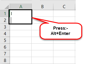
- Step #3 – We can see that it inserted a line break after I. Now, do this for every word.
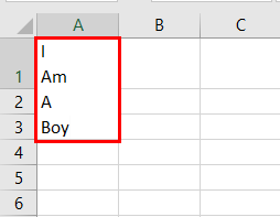
- Step #4 – Press the “Enter” key and see the result.
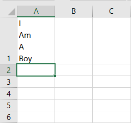
We have successfully inserted a line break using the “Alt + Enter” method.
Things to Remember
There are a few things we need to remember in line breaks:
- To use AND and CONCATENATE functions, we must wrap text to view the whole data.
- We must expand the rows after wrapping the text.
- The CHAR (10) function inserts a line break.
- The “Alt + Enter” method works in a single cell. However, for it to work in another cell, we must repeat the process.
Recommended Articles
This article is a guide to Line Break in Excel Cell. We discuss how to insert a line break in Excel using 1) AND Formula, 2) CONCATENATE Formula, and 3) Alt + Enter method, along with practical examples and a downloadable template. You may learn more about Excel from the following articles: –
- BreakPoint in VBA
- Excel Concatenate Columns
- Concatenate Function in VBA
- Format Phone Numbers in Excel