
Excel for Microsoft 365 Excel 2021 Excel 2019 Excel 2016 Excel 2013 Excel 2010 Excel 2007 Excel Starter 2010 More…Less
When you want to display a list of values that users can choose from, add a list box to your worksheet.
Add a list box to a worksheet
-
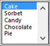
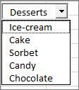
Create a list of items that you want to displayed in your list box like in this picture.

-
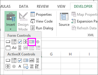
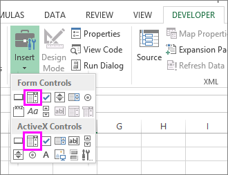
Click Developer > Insert.
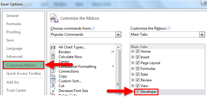
Note: If the Developer tab isn’t visible, click File > Options > Customize Ribbon. In the Main Tabs list, check the Developer box, and then click OK.
-
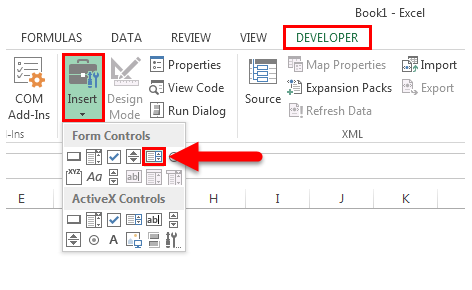
Under Form Controls, click List box (Form Control).
-
Click the cell where you want to create the list box.
-
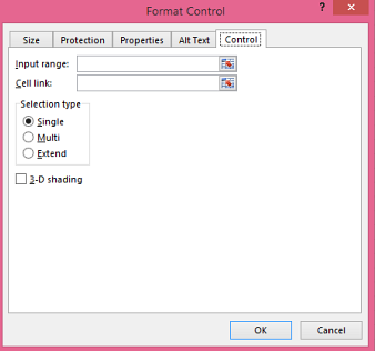
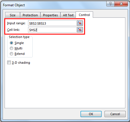
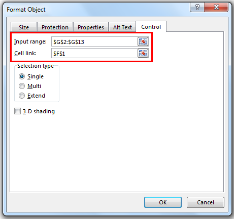
Click Properties > Control and set the required properties:
-
In the Input range box, type the range of cells containing the values list.
Note: If you want more items displayed in the list box, you can change the font size of text in the list.
-
In the Cell link box, type a cell reference.
Tip: The cell you choose will have a number associated with the item selected in your list box, and you can use that number in a formula to return the actual item from the input range.
-
Under Selection type, pick a Single and click OK.
Note: If you want to use Multi or Extend, consider using an ActiveX list box control.
-
Add a combo box to a worksheet
You can make data entry easier by letting users choose a value from a combo box. A combo box combines a text box with a list box to create a drop-down list.
You can add a Form Control or an ActiveX Control combo box. If you want to create a combo box that enables the user to edit the text in the text box, consider using the ActiveX Combo Box. The ActiveX Control combo box is more versatile because, you can change font properties to make the text easier to read on a zoomed worksheet and use programming to make it appear in cells that contain a data validation list.
-
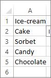
Pick a column that you can hide on the worksheet and create a list by typing one value per cell.
Note: You can also create the list on another worksheet in the same workbook.
-
Click Developer > Insert.
Note: If the Developer tab isn’t visible, click File > Options > Customize Ribbon. In the Main Tabs list, check the Developer box, and then click OK.
-
Pick the type of combo box you want to add:
-
Under Form Controls, click Combo box (Form Control).
Or
-
Under ActiveX Controls, click Combo Box (ActiveX Control).
-
-
Click the cell where you want to add the combo box and drag to draw it.
Tips:
-
To resize the box, point to one of the resize handles, and drag the edge of the control until it reaches the height or width you want.
-
To move a combo box to another worksheet location, select the box and drag it to another location.
Format a Form Control combo box
-
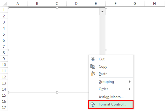
Right-click the combo box and pick Format Control.
-
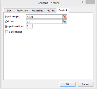
Click Control and set the following options:
-
Input range: Type the range of cells containing the list of items.
-
Cell link: The combo box can be linked to a cell where the item number is displayed when you select an item from the list. Type the cell number where you want the item number displayed.
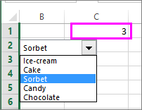
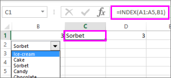
For example, cell C1 displays 3 when the item Sorbet is selected, because it’s the third item in our list.
Tip: You can use the INDEX function to show an item name instead of a number. In our example, the combo box is linked to cell B1 and the cell range for the list is A1:A2. If the following formula, is typed into cell C1: =INDEX(A1:A5,B1), when we select the item «Sorbet» is displayed in C1.
-
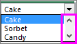
Drop-down lines: The number of lines you want displayed when the down arrow is clicked. For example, if your list has 10 items and you don’t want to scroll you can change the default number to 10. If you type a number that’s less than the number of items in your list, a scroll bar is displayed.
-
-
Click OK.
Format an ActiveX combo box
-
Click Developer > Design Mode.
-
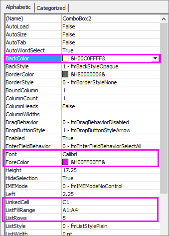
Right-click the combo box and pick Properties, click Alphabetic, and change any property setting that you want.
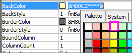
Here’s how to set properties for the combo box in this picture:
To set this property
Do this
Fill color
Click BackColor > the down arrow > Pallet, and then pick a color.
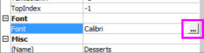
Font type, style or size
Click Font > the… button and pick font type, size, or style.
Font color
Click ForeColor > the down arrow > Pallet, and then pick a color.
Link a cell to display selected list value.
Click LinkedCell
Link Combo Box to a list
Click the box next to ListFillRange and type the cell range for the list.
Change the number of list items displayed
Click the ListRows box and type the number of items to be displayed.
-
Close the Property box and click Designer Mode.
-
After you complete the formatting, you can right-click the column that has the list and pick Hide.
Need more help?
You can always ask an expert in the Excel Tech Community or get support in the Answers community.
See Also
Overview of forms, Form controls, and ActiveX controls on a worksheet
Add a check box or option button (Form controls)
Need more help?
Want more options?
Explore subscription benefits, browse training courses, learn how to secure your device, and more.
Communities help you ask and answer questions, give feedback, and hear from experts with rich knowledge.
The list box in Excel (Table of Contents)
- List box in Excel
- How to Create List box in Excel?
- Examples of the List box in Excel
List Box in Excel
List Box in excel is used to create a list inside the box and choose them just we select the values from dropdown. List boxes are available in the Insert option in the Developer menu tab. We can use List boxes with VBA macro and also excel cells. Whatever values we select can be seen in the list box, and once we select any value that will be reflected, the cell linked to List Box.
List Box is located under Developer Tab in Excel. If you are not a VBA macro user, you may not see this DEVELOPER tab in your excel.
Follow the below steps to unleash the Developer Tab.
If the Developer tab is not showing, then follow the below steps to enable the Developer tab.
- Go to the FILE option (top of the left-hand side of the excel).
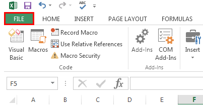
- Now go to Options.
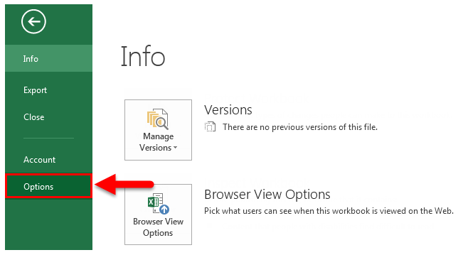
- Go to Custom Ribbon and click on the Developer tab check-box.
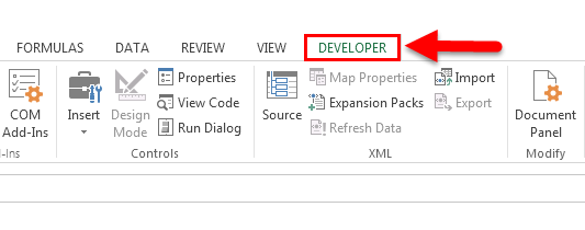
- Once the Developer Tab is enabled, you can see it on your excel ribbon.
How to Create List box in Excel?
Follow the below steps to insert the List box in excel.
You can download this List Box Excel Template here – List Box Excel Template
Step 1: Go to Developer Tab > Controls > Insert > Form Controls > List Box.
Step 2: Click on List Box and draw in the worksheet; then Right-click on the List Box and select the option Format Control.
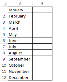
Step 3: Create a month list in column A from A1 to A12.
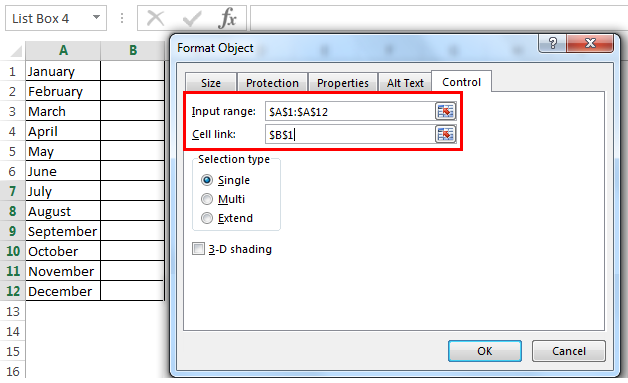
Step 4: Once you have selected Format Control, it will open the below dialog box; go to the Control tab in the input range select the month lists from A1 to A10. In the cell link, give a link to cell B1.
We have linked our cell to B1. Once the first value has selected the cell B1 will show 1. Similarly, if you select April, it will show 4 in cell B1.
Examples of List Box in Excel
Let’s look at a few examples of using Lise Box in Excel.
Example #1 – List Box with Vlookup Formula
Now we will look at the way of using List Box in excel.
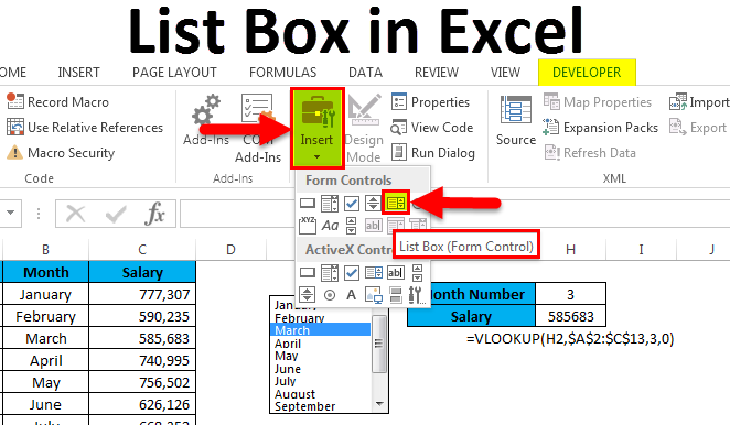
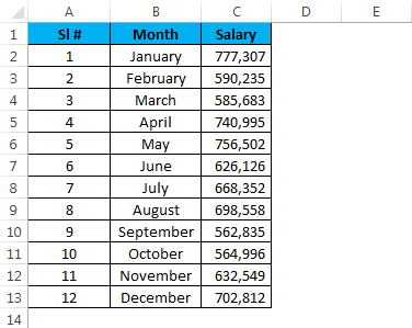
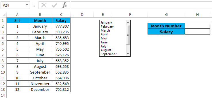
Assume you have salary data month-wise from A2 to A13. Based on the selection made from the list, it has to show the value for the selected month.
Step 1: Draw a List Box from the developer tab and create a list of months.
Step 2: I have given a cell link to H2. In G2 and G3, create a list like this.
Step 3: Apply the VLOOKUP formula in cell H3 to get the salary data from the list.
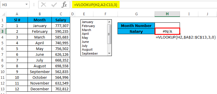
Step 4: Right now, it is showing an error as #N/A. Please select any of the months; it will show you the salary data for that month.
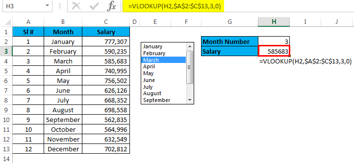
I have selected March month, and the number for March month is 3 and VLOOKUP showing the value for number 3 from the table.
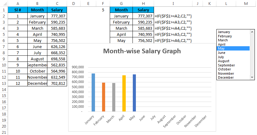
Example #2 – Custom Chart with List Box
In this example, I will explain how to create the custom chart using List Box. I will take the same example that I have used previously.
Step 1: Create a table like this.
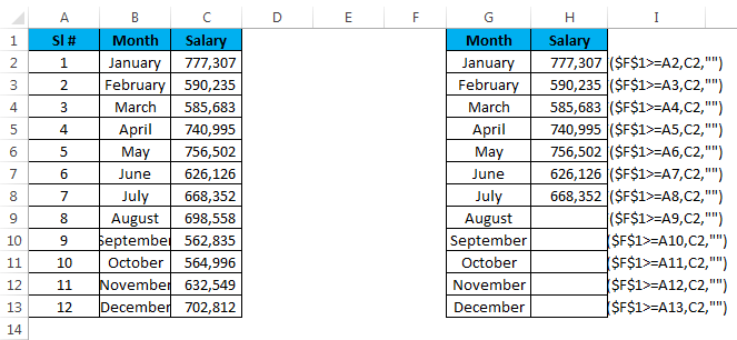
Step 2: Insert List Box from the Developer tab. Go to Format Control give a link to the month list and a cell link to F1.
Step 3: Apply the IF formula in the newly created table.
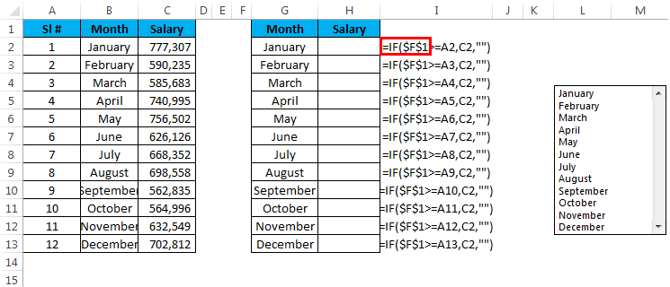
I have applied the IF condition to the table. If I select the month March, the value in cell F1 will show the number 3 because March is the third value in the list. Similarly, it will show 4 for April, 10 for October and 12 for December.
IF condition checks if the value in the cell F1 is greater than equal to 4, it will show for the value for the first 4 months. If the value in cell F1 is greater than equal to 6, it will show the value for the first 6 months only.
Step 4: Now apply the chart for the modified table with the IF condition.
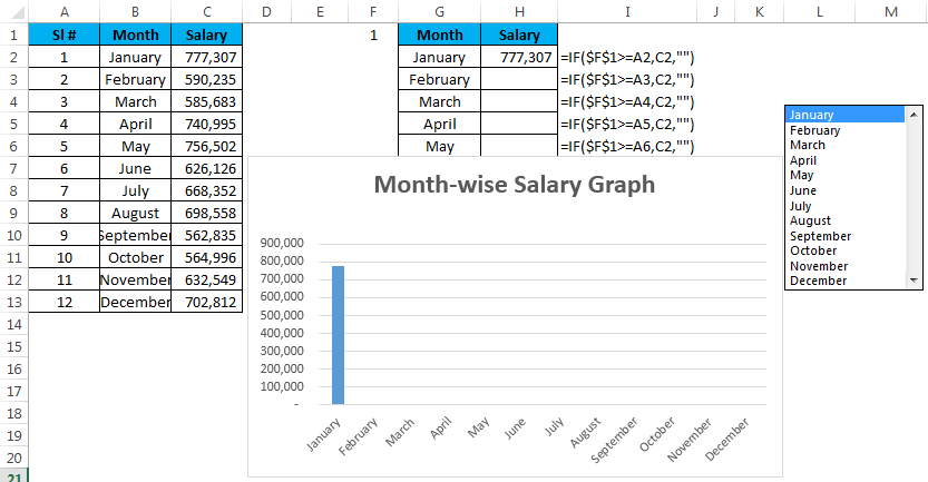
Step 5: Now it is showing the empty graph. Select the month to see the magic. I have selected the month of May, which is why it shows the graph for the first 5 months.
Things to Remember
- There is one more List Box under Active X Control in excel. This has mainly used in VBA macros.
- Cell link is to indicate which item from the list has selected.
- We can control the user to enter the data by using List Box.
- We can avoid wrong data entry by using List Box.
Recommended Articles
This has been a guide to the List box in Excel. Here we discuss the List box in Excel and How to create the List box in Excel along with practical examples and a downloadable excel template. You can also go through our other suggested articles –
- Name Box in Excel
- Excel Search Box
- CheckBox in Excel
- Compare Two Lists in Excel
Microsoft Excel has a functionality where we can link a textbox to a specific cell. If we change the data in the cell, the value of the linked cell gets updated automatically. Below are the following steps to link a cell to a text box:
1. Open Excel
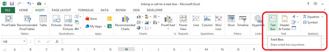
2. Click on the Insert tab
3. Click the Text Box button
4. A text Box will Open

5. Select the Text Box
6. Type = in the Formula Bar
7. Select the cell where you want to give a reference
Let us take an example
1. Open Excel
2. Click on the Insert tab
3. Click the Text Box button
4. A text Box will Open
5. Select the Text Box
6. Type = in the Formula Bar
7. Select the cell A1

8. After we select Cell A1, automatically it will display “=$A$1”
9. Now when we change the Text in cell A1, automatically text in the Text Box will change

There are several different methods for selecting a block of cells in Excel, or extending an existing selection with more cells. Let’s take a look at them.
Select a Range of Cells By Clicking and Dragging
One of the easiest ways to select a range of cells is by clicking and dragging across the workbook.
Click the first cell you want to select and continue holding down your mouse button.

Drag your pointer over all the cells you want in the selection, and then release your mouse button.
You should now have a group of cells selected.
Select a Large Range of Cells With the Shift Key
Sometimes, clicking and dragging isn’t convenient because the range of cells you want to select extends off your screen. You can select a range of cells using your Shift key, much the same way you’d select a group of files in a file folder.
Click the first cell in the range you want to select.
Scroll your sheet until you find the last cell in the range you want to select. Hold down your Shift key, and then click that cell.
All the cells in the range are now selected.
Select (or Deselect) Independent Cells Outside a Range With the Ctrl Key
You can also select multiple cells that are not connected to one another by using your Ctrl key.
Click the first cell you want to select.
Now, hold down the Ctrl key and click to select additional cells. In the image below, we’ve selected five different cells.
You can also use your Ctrl key to deselect an already selected cell—even from a selection range. In the image below, we deselected several cells from a range of cells we’d already selected just by holding down the Ctrl key while clicking the cells.
Select a Range of Cells Using the Name Box
If you know the exact range of cells you want to select, using the name box is a useful way to make the selection without any clicking or dragging.
Click the name box in the top left of the workbook.
Type in the range of cells you want to select using the following format:
First Cell:LastCell
Here, we’re selecting all the cells from cell B2 (our top left cell) to F50 (our bottom right cell).
Hit Enter (or Return on Mac), and the cells you input are selected.
Select an Entire Row of Cells
You may need to select an entire row of cells at one time—perhaps to apply formatting a header row. It’s easy to do this.
Just click the row number at the left hand side of the row.
The entire row is now selected.
Select Multiple Entire Rows of Cells.
Sometimes, you may want to select multiple entire rows cells. Much like with selecting individual cells, you’ll use the Shift key if the rows are contiguous (or you can click and drag) and the Ctrl key if the rows are noncontiguous.
To select a contiguous set of rows, click the row number of the first row.
Continuing to hold down your mouse button, drag your cursor across all the rows you want to select. Or, if you prefer, you can hold down your Shift key and click the bottom-most row you want to select. Either way, you’ll select a range of rows.
To select noncontiguous rows, click the row number of a row you want to select.
Then hold down your Ctrl key while clicking the row numbers of additional rows you want to add to the selection. In the image below, we’ve selected several rows that are noncontiguous.
And, just like with individual cells, you can also use the Ctrl key to deselect rows from a selected range. In the image below, we’ve deselected two rows from a selected range by holding down the Ctrl key while clicking the row numbers of the rows we didn’t want in the selection.
Select One or More Entire Columns of Cells
Sometimes, you may want to select an entire column of cells. It’s easy to do this, too. In fact, it works exactly like selecting rows.
Click a column letter to select the column.
You can also select multiple columns by clicking and dragging or by using the Shift key, just like with rows. The Ctrl key also works for selecting noncontiguous columns or for deselecting columns from a selected range.
READ NEXT
- › How to Set the Print Area in Microsoft Excel
- › How to Use an Advanced Filter in Microsoft Excel
- › How to Create and Customize a Treemap Chart in Microsoft Excel
- › How to Create and Customize a Funnel Chart in Microsoft Excel
- › How to Add or Subtract Times in Microsoft Excel
- › How to Format Phone Numbers in Microsoft Excel
- › How to Move Cells in Microsoft Excel
- › BLUETTI Slashed Hundreds off Its Best Power Stations for Easter Sale
- Column
- TECHNOLOGY Q&A
By J. Carlton Collins, CPA
Q. Is it possible to link the contents of a text box in Excel to data in a cell?
A. Yes, you can link the contents of an Excel text box to data in a cell as follows:
1. Insert a text box. Insert a text box in Excel from the Insert tab by selecting Text, Text Box, and then use your mouse to drag to a region on your worksheet.

2. Insert a formula in the text box. With the Text Box still selected, press the F2 key. This will activate the formula bar (indicated by a blinking cursor in the formula bar). Write your desired formula (in the example shown above, I entered the formula =B2) and press Enter. Thereafter, the text box will display the data contained in the linked cell (405,843 in this example), even if the contents of that cell change.
Additional comments about text boxes:
a. The linked text box will continue to work even if you move it to another worksheet or to another workbook.
b. The linked text box will work even if you create the link in a different worksheet or workbook.
c. This type of link also works with other shapes, such as the four example speech bubbles pictured below. (In this screenshot, I also applied a few of the available formatting effects involving colors, shadows, bevels, and glow effects.)

d. With a little tech-savvy trickery, it is possible to combine text and numbers to embed a full sentence in a text box or speech bubble. For example, below in cell A4, I have used the Concatenate symbol (the «&» symbol) to combine both text and numbers. I also used the Text function to control the formatting of the values included in the sentence. I then embedded the resulting formula in the speech bubble and included a clip art image of myself. The result is an image with a speech bubble that changes automatically as the values in the worksheet change.
This type of effect may be useful in certain situations to help emphasize key results produced in a workbook. You can download this example workbook at carltoncollins.com/textbox.xlsx.

About the author
J. Carlton Collins (carlton@asaresearch.com) is a technology consultant, a CPE instructor, and a JofA contributing editor.
Note: Instructions for Microsoft Office in “Technology Q&A” refer to the 2007 through 2016 versions, unless otherwise specified.
Submit a question
Do you have technology questions for this column? Or, after reading an answer, do you have a better solution? Send them to jofatech@aicpa.org. We regret being unable to individually answer all submitted questions.