
This page is a guide to creating your own option pricing Excel spreadsheet, in line with the Black-Scholes model (extended for dividends by Merton). Here you can get a ready-made Black-Scholes Excel calculator with charts and additional features such as parameter calculations and simulations.
Black-Scholes in Excel: The Big Picture
If you are not familiar with the Black-Scholes model, its assumptions, parameters, and (at least the logic of) the formulas, you may want to read those pages first (overview of all Black-Scholes resources is here).
Below I will show you how to apply the Black-Scholes formulas in Excel and how to put them all together in a simple option pricing spreadsheet. There are four steps:
- Design cells where you will enter parameters.
- Calculate d1 and d2.
- Calculate call and put option prices.
- Calculate option Greeks.
Black-Scholes Inputs

First you need to design six cells for the six Black-Scholes parameters. When pricing a particular option, you will have to enter all the parameters in these cells in the correct format. The parameters and formats are:
S = underlying price (USD per share)
K = strike price (USD per share)
σ = volatility (% p.a.)
r = continuously compounded risk-free interest rate (% p.a.)
q = continuously compounded dividend yield (% p.a.)
t = time to expiration (% of year)
Underlying price is the price at which the underlying security is trading on the market at the moment you are doing the option pricing. Enter it in dollars (or euros/yen/pound etc.) per share.
Strike price, also called exercise price, is the price at which you will buy (if call) or sell (if put) the underlying security if you choose to exercise the option. If you need more explanation, see: Strike vs. Market Price vs. Underlying Price. Enter it also in dollars per share (it must have same units as underlying price, also with the same contract or lot multipliers).
Volatility is the most difficult parameter to estimate (all the other parameters are more or less given). It is your job to decide how high volatility you expect and what number to enter – neither the Black-Scholes model, nor this page will tell you how high volatility to expect with your particular option (for more on that, see the volatility tutorials, particularly historical and implied volatility). Being able to estimate (= predict) volatility with more success than other people is the hard part and key factor determining success or failure in option trading. The important thing here is to enter it in the correct format, which is % p.a. (percent annualized).
Risk-free interest rate should be entered in % p.a., continuously compounded. The interest rate’s tenor (time to maturity) should match the time to expiration of the option you are pricing. You can interpolate the yield curve to get the interest rate for your exact time to expiration. Interest rate does not affect the resulting option price very much in the low interest environment that we’ve had in the recent years, but it can become very important when rates are higher (for more details on the effect of interest rates on option prices see the option rho tutorial).
Dividend yield should also be entered in % p.a., continuously compounded. If the underlying stock doesn’t pay any dividend, enter zero. If you are pricing an option on securities other than stocks, you may enter the second country interest rate (for FX options) or convenience yield (for commodities) here.
Time to expiration should be entered as % of year between the moment of pricing (now) and expiration of the option. For example, if the option expires in 24 calendar days, enter 24/365 = 6.58%. Alternatively, you can measure time in trading days rather than calendar days. If the option expires in 18 trading days and there are 252 trading days per year, you will enter time to expiration as 18/252 = 7.14%. You can also be more precise and measure time to expiration to hours or even minutes. In any case you must always express the time to expiration as % of year in order for the calculations to return correct results (it is very easy in Excel – just divide the number of days to expiration by the number of days per year).
I will illustrate the calculations on the example below. The parameters are in cells A44 (underlying price), B44 (strike price), C44 (volatility), D44 (interest rate), E44 (dividend yield), and G44 (time to expiration as % of year).

Note: It is row 44, because I am using the Black-Scholes Calculator for screenshots and it has charts in the rows above. You can of course start in row 1 or arrange your calculations in a column.
Black-Scholes d1 and d2
When you have the cells with parameters ready, the next step is to calculate d1 and d2, because these terms then enter all the calculations of call and put option prices and Greeks. The formulas for d1 and d2 are:


All the operations in these formulas are relatively simple mathematics. The only things that may be unfamiliar to some less savvy Excel users are the natural logarithm (LN Excel function) and square root (SQRT Excel function).
The hardest thing with the d1 formula is making sure you put the brackets in the right places. This is why you may want to calculate individual parts of the formula in separate cells, as I do in the example below:

First I calculate the natural logarithm of the ratio of underlying price and strike price (this is why they must have the same units) in cell H44:
=LN(A44/B44)
Then I calculate the rest of the numerator of the d1 formula in cell I44:
=(D44-E44+POWER(C44,2)/2)*G44
Then I calculate the denominator of the d1 formula in cell J44. Another reason why you may want to calculate d1 in separate parts is that this term will also enter the formula for d2:
=C44*SQRT(G44)
Now I have all the three parts of the d1 formula and I can combine them in cell K44 to get d1:
=(H44+I44)/J44
Finally, I calculate d2 in cell L44:
=K44-J44
Black-Scholes Option Price Excel Formulas
The Black-Scholes formulas for call option (C) and put option (P) prices are:


The two formulas are very similar. There are four terms in each formula. I will again calculate them in separate cells first and then combine them in the final call and put formulas.
N(d1), N(d2), N(-d2), N(-d1)
Potentially unfamiliar parts of the formulas are the N(d1), N(d2), N(-d2), and N(-d1) terms.
N(x) denotes the standard normal cumulative distribution function:
")
For example, N(d1) is the standard normal cumulative distribution function for the d1 that we have calculated in the previous step.
In Excel you can easily calculate the standard normal cumulative distribution functions using the NORM.DIST function, which has four parameters:
NORM.DIST(x, mean, standard_dev, cumulative)- x = link to the cell where you have calculated d1 or d2 (with minus sign for -d1 and -d2)
- mean = enter 0, because it is standard normal distribution
- standard_dev = enter 1, because it is standard normal distribution
- cumulative = enter TRUE, because it is cumulative
For example, I calculate N(d1) in cell M44:
=NORM.DIST(K44,0,1,TRUE)
Note: There is also the NORM.S.DIST function in Excel, which is the same as NORM.DIST with fixed mean = 0 and standard_dev = 1 (therefore you enter only two parameters: x and cumulative). You can use either. NORM.S.DIST may not be available in some spreadsheet software.
The Terms with Exponential Functions
The exponents (e-qt and e-rt terms) are calculated using the EXP Excel function with -q*t or -r*t as parameter.
I calculate e-rt in cell Q44:
=EXP(-D44*G44)
Then I use it to calculate K e-rt in cell R44:
=B44*Q44
Analogically, I calculate e-qt in cell S44:
=EXP(-E44*G44)
Then I use it to calculate S e-qt in cell T44:
=A44*S44
Now I have all the individual terms and I can calculate the final call and put option price.
Call Option Price
I combine the four terms in the call formula to get call option price in cell U44:
=T44*M44-R44*O44
Put Option Price
I combine the four terms in the put formula to get put option price in cell U44:
=R44*P44-T44*N44
Black-Scholes Greeks in Excel

Here you can continue to the second part of this tutorial, which explains Excel calculation of the Greeks: delta, gamma, theta, vega, and rho:
Continue to Option Greeks Excel Formulas
Or you can see how all the Excel calculations work together in the Black-Scholes Calculator. Explanation of the calculator’s other features (parameter calculations and simulations of option prices and Greeks) are available in the calculator’s user guide.
Содержание
- How to Use Excel to Simulate Stock Prices
- Key Takeaways
- Building a Pricing Model Simulation
- Black-Scholes option pricing in Excel and VBA
- 1. Black-Scholes model
- 2. The Black-Scholes model in Excel
- 3. The Black-Scholes model in VBA
- References
- Related material
- Black-Scholes Excel Formulas and How to Create a Simple Option Pricing Spreadsheet
- Black-Scholes in Excel: The Big Picture
- Black-Scholes Inputs
- Black-Scholes d1 and d2
- Black-Scholes Option Price Excel Formulas
- N(d1), N(d2), N(-d2), N(-d1)
- The Terms with Exponential Functions
- Call Option Price
- Put Option Price
- Black-Scholes Greeks in Excel
How to Use Excel to Simulate Stock Prices
:max_bytes(150000):strip_icc()/picture-53711-1421794744-5bfc2a9246e0fb005119864b.jpg)
Some active investors model variations of a stock or other asset to simulate its price and that of the instruments that are based on it, such as derivatives. Simulating the value of an asset on an Excel spreadsheet can provide a more intuitive representation of its valuation for a portfolio.
Key Takeaways
- Traders looking to back-test a model or strategy can use simulated prices to validate its effectiveness.
- Excel can help with your back-testing using a monte carlo simulation to generate random price movements.
- Excel can also be used to compute historical volatility to plug into your models for greater accuracy.
Building a Pricing Model Simulation
Whether we are considering buying or selling a financial instrument, the decision can be aided by studying it both numerically and graphically. This data can help us judge the next likely move that the asset might make and the moves that are less likely.
First of all, the model requires some prior hypotheses. We assume, for example, that the daily returns, or «r(t),» of these assets are normally distributed with the mean, «(μ),» and standard deviation sigma, «(σ).» These are the standard assumptions that we will use here, though there are many others that could be used to improve the accuracy of the model.
Источник
Black-Scholes option pricing in Excel and VBA
1. Black-Scholes model
According to the Black-Scholes (1973) model, the theoretical price (C) for European call option on a non dividend paying stock is $$begin C=S_0 N(d_1)-Xe^<-rT>N(d_2) end$$ where $$d_1=frac right) + left( r+ frac <sigma^2> <2>right )T><sigma sqrt> $$ $$d_2=frac right) + left( r — frac <sigma^2> <2>right )T><sigma sqrt> = d_1 — sigma sqrt$$
In equation 1, (S_0) is the stock price at time 0, (X) is the exercise price of the option, (r) is the risk free interest rate, (sigma) represents the annual volatility of the underlying asset, and (T) is the time to expiration of the option.
From Put-Call parity, the theoretical price (P) of European put option on a non dividend paying stock is $$begin P=Xe^<-rT>N(-d_2) — S_0 N(-d_1) end$$
2. The Black-Scholes model in Excel
Example: The stock price at time 0, six months before expiration date of the option is $42.00, option exercise price is $40.00, the rate of interest on a government bond with 6 months to expiration is 5%, and the annual volatility of the underlying stock is 20%.
The values used in this example are similar to those in Hull (2009, p294 ) with S0 = 42, K (exercise) = 40, r = 0.1, σ = 0.2, and T = 0.5. This set returns c = 4.76 and p = 0.81
Calculation of the call price can be completed as a 5 step process. Step 1. d1; 2. d2 as ( left[frac right) + left( r — frac <sigma^2> <2>right )T><sigma sqrt> right]); 3. N(d1); 4. N(d2); and step 5, C. The value for d1 and d2 are shown in rows 12 and 13 of figure 1. The probabilities for (N(cdot)) are estimated with the NORM.S.DIST function. The call price from equation 1 is $4.08 (Figure 1 row 18), and the put price from equation 2 is $1.09 (Figure 1 row 19).
Syntax NORM.S.DIST(z,cumulative) . z is the probability value, and cumulative is a LOGICAL value. TRUE returns the cumulative distribution function. FALSE returns the probability mass function.
Fig 1: Excel Web App #1: — Excel version of Black and Scholes’ model for a European type option on a non dividend paying stock
3. The Black-Scholes model in VBA
In this example, separate function procedures are developed for the call (code 1) and put (code 2) equations. The Excel NORM.S.DIST function, line 6 in code 1 and 2, requires that the dot operators be replaced by underscores when the function is called from VBA.
The BScall and BSPut functions are tested by the calling procedure in code 3. Output is sent to the Immediate Window with the Debug.Print method.
The output from code 3 is shown in the Immediate Window of figure 2.
 Fig 2: Black and Scholes’ model — for a European type option on a non dividend paying stock
A combination Call and Put procedure is shown in Code 4.
The BSOption function functions is tested by the calling procedure in code 5.
References
Black F, and M Scholes, (1973), The pricing of options and corporate liabilities, Journal of Political Economy, Vol 81 No 3 pp.637-654.
Hull J, (2009), ‘Options, futures, and other derivatives’, 7th ed., Pearson Prentice Hall
Black Scholes on the HP10bII+ financial calculator
Social media links
Added 24th February 2016
- Download the Excel file for this module: bs_nondiv.xlsm [29 KB]
- Download the VBA code for this module: xlf-black-scholes-code.txt [4 KB]
- Development platform: Microsoft Excel 2013 Pro 64 bit.
- Revised: Friday 24th of February 2023 — 10:37 PM, Pacific Time (PT)
Copyright © 2011 – 2023 ♦ Dr Ian O’Connor, CPA. | Privacy policy
Источник
Black-Scholes Excel Formulas and How to Create a Simple Option Pricing Spreadsheet
This page is a guide to creating your own option pricing Excel spreadsheet, in line with the Black-Scholes model (extended for dividends by Merton). Here you can get a ready-made Black-Scholes Excel calculator with charts and additional features such as parameter calculations and simulations.
Black-Scholes in Excel: The Big Picture
If you are not familiar with the Black-Scholes model, its assumptions, parameters, and (at least the logic of) the formulas, you may want to read those pages first (overview of all Black-Scholes resources is here).
Below I will show you how to apply the Black-Scholes formulas in Excel and how to put them all together in a simple option pricing spreadsheet. There are four steps:
- Design cells where you will enter parameters.
- Calculate d1 and d2.
- Calculate call and put option prices.
- Calculate option Greeks.
Black-Scholes Inputs
First you need to design six cells for the six Black-Scholes parameters. When pricing a particular option, you will have to enter all the parameters in these cells in the correct format. The parameters and formats are:
S = underlying price (USD per share)
K = strike price (USD per share)
σ = volatility (% p.a.)
r = continuously compounded risk-free interest rate (% p.a.)
q = continuously compounded dividend yield (% p.a.)
t = time to expiration (% of year)
Underlying price is the price at which the underlying security is trading on the market at the moment you are doing the option pricing. Enter it in dollars (or euros/yen/pound etc.) per share.
Strike price, also called exercise price, is the price at which you will buy (if call) or sell (if put) the underlying security if you choose to exercise the option. If you need more explanation, see: Strike vs. Market Price vs. Underlying Price. Enter it also in dollars per share (it must have same units as underlying price, also with the same contract or lot multipliers).
Volatility is the most difficult parameter to estimate (all the other parameters are more or less given). It is your job to decide how high volatility you expect and what number to enter – neither the Black-Scholes model, nor this page will tell you how high volatility to expect with your particular option (for more on that, see the volatility tutorials, particularly historical and implied volatility). Being able to estimate (= predict) volatility with more success than other people is the hard part and key factor determining success or failure in option trading. The important thing here is to enter it in the correct format, which is % p.a. (percent annualized).
Risk-free interest rate should be entered in % p.a., continuously compounded. The interest rate’s tenor (time to maturity) should match the time to expiration of the option you are pricing. You can interpolate the yield curve to get the interest rate for your exact time to expiration. Interest rate does not affect the resulting option price very much in the low interest environment that we’ve had in the recent years, but it can become very important when rates are higher (for more details on the effect of interest rates on option prices see the option rho tutorial).
Dividend yield should also be entered in % p.a., continuously compounded. If the underlying stock doesn’t pay any dividend, enter zero. If you are pricing an option on securities other than stocks, you may enter the second country interest rate (for FX options) or convenience yield (for commodities) here.
Time to expiration should be entered as % of year between the moment of pricing (now) and expiration of the option. For example, if the option expires in 24 calendar days, enter 24/365 = 6.58%. Alternatively, you can measure time in trading days rather than calendar days. If the option expires in 18 trading days and there are 252 trading days per year, you will enter time to expiration as 18/252 = 7.14%. You can also be more precise and measure time to expiration to hours or even minutes. In any case you must always express the time to expiration as % of year in order for the calculations to return correct results (it is very easy in Excel – just divide the number of days to expiration by the number of days per year).
I will illustrate the calculations on the example below. The parameters are in cells A44 (underlying price), B44 (strike price), C44 (volatility), D44 (interest rate), E44 (dividend yield), and G44 (time to expiration as % of year).
Note: It is row 44, because I am using the Black-Scholes Calculator for screenshots and it has charts in the rows above. You can of course start in row 1 or arrange your calculations in a column.
Black-Scholes d1 and d2
When you have the cells with parameters ready, the next step is to calculate d1 and d2, because these terms then enter all the calculations of call and put option prices and Greeks. The formulas for d1 and d2 are:
All the operations in these formulas are relatively simple mathematics. The only things that may be unfamiliar to some less savvy Excel users are the natural logarithm ( LN Excel function) and square root ( SQRT Excel function).
The hardest thing with the d1 formula is making sure you put the brackets in the right places. This is why you may want to calculate individual parts of the formula in separate cells, as I do in the example below:
First I calculate the natural logarithm of the ratio of underlying price and strike price (this is why they must have the same units) in cell H44:
Then I calculate the rest of the numerator of the d1 formula in cell I44:
Then I calculate the denominator of the d1 formula in cell J44. Another reason why you may want to calculate d1 in separate parts is that this term will also enter the formula for d2:
Now I have all the three parts of the d1 formula and I can combine them in cell K44 to get d1:
Finally, I calculate d2 in cell L44:
Black-Scholes Option Price Excel Formulas
The Black-Scholes formulas for call option (C) and put option (P) prices are:
The two formulas are very similar. There are four terms in each formula. I will again calculate them in separate cells first and then combine them in the final call and put formulas.
N(d1), N(d2), N(-d2), N(-d1)
N(x) denotes the standard normal cumulative distribution function:
For example, N(d1) is the standard normal cumulative distribution function for the d1 that we have calculated in the previous step.
In Excel you can easily calculate the standard normal cumulative distribution functions using the NORM.DIST function, which has four parameters:
- x = link to the cell where you have calculated d1 or d2 (with minus sign for -d1 and -d2)
- mean = enter 0, because it is standard normal distribution
- standard_dev = enter 1, because it is standard normal distribution
- cumulative = enter TRUE, because it is cumulative
For example, I calculate N(d1) in cell M44:
Note: There is also the NORM.S.DIST function in Excel, which is the same as NORM.DIST with fixed mean = 0 and standard_dev = 1 (therefore you enter only two parameters: x and cumulative). You can use either. NORM.S.DIST may not be available in some spreadsheet software.
The Terms with Exponential Functions
The exponents (e -qt and e -rt terms) are calculated using the EXP Excel function with -q*t or -r*t as parameter.
I calculate e -rt in cell Q44:
Then I use it to calculate K e -rt in cell R44:
Analogically, I calculate e -qt in cell S44:
Then I use it to calculate S e -qt in cell T44:
Now I have all the individual terms and I can calculate the final call and put option price.
Call Option Price
I combine the four terms in the call formula to get call option price in cell U44:
Put Option Price
I combine the four terms in the put formula to get put option price in cell U44:
Black-Scholes Greeks in Excel
Here you can continue to the second part of this tutorial, which explains Excel calculation of the Greeks: delta, gamma, theta, vega, and rho:
Or you can see how all the Excel calculations work together in the Black-Scholes Calculator. Explanation of the calculator’s other features (parameter calculations and simulations of option prices and Greeks) are available in the calculator’s user guide.
Источник
Simplified
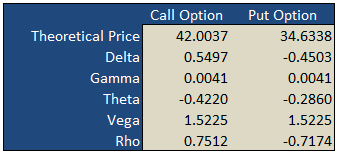
On the «basic» worksheet tab you will find a simple option calculator that generates fair values and option Greeks for a single call and put according to the underlying inputs you select. The white areas are for your user input while the shaded green areas are the model outputs.
Implied Volatility
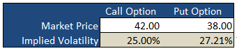
Underneath the main pricing outputs is a section for calculating the implied volatility for the same call and put option. Here, you enter the market prices for the options, either last paid or bid/ask into the white Market Price cell and the spreadsheet will calculate the volatility that the model would have used to generate a theoretical price that is in-line with the market price i.e. the «implied» volatility.
Payoff Graphs
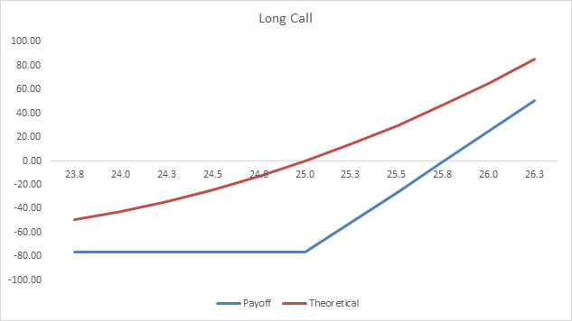
The PayoffGraphs tab gives you the profit and loss profile of basic option legs; buy call, sell call, buy put and sell put. You can change the underlying inputs to see how your changes effect the profit profile of each option.
Strategies
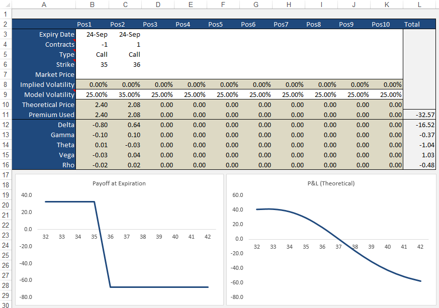
The Strategies tab allows you to create option/stock combinations of up to 10 components. Again, use the while areas for your user input while the shaded areas are for the model outputs.
Formulas
Theoretical and Greek Prices
Use this Excel formula for generating theoretical prices for either call or put as well as the option Greeks:
=OTW_BlackScholes(Type, Output, Underlying Price, Exercise Price, Time, Interest Rates, Volatility, Dividend Yield)
- Type
- c = Call, p = Put, s = Stock
- Output
- p = theoretical price, d = delta, g = gamma, t = theta, v = vega, r = rho
- Underlying Price
- The current market price of the stock
- Exercise Price
- The exercise/strike price of the option
- Time
- Time to expiration in years e.g. 0.50 = 6 months
- Interest Rates
- As a percentage e.g. 5% = 0.05
- Volatlity
- As a percentage e.g. 25% = 0.25
- Dividend Yield
- As a percentage e.g. 4% = 0.04
A Sample formula would look like =OTW_BlackScholes(c, p, 25, 26, 0.25, 0.05, 0.21, 0.015).
Implied Volatility
=OTW_IV(Type, Underlying Price, Exercise Price, Time, Interest Rates, Market Price, Dividend Yield)
Same inputs as above except:
- Market Price
- The current market last, bid/ask of the option
Example: =OTW_IV(p, 100, 100, 0.74, 0.05, 8.2, 0.01)
Support
If you’re having troubles getting the formulas to work, please check out the support page or send me an email.
If you’re after an online version of an option calculator then you should visit Option-Price.com
Just to note that much of what I have learnt that made this spreadsheet possible was taken from the highly acclaimed book on financial modeling by Simon Benninga — Financial Modeling — 3rd Edition ![]()
![]()
If you’re an Excel junkie, you’ll love this book. There are loads of real world problems that Simon solves using Excel. The book also comes with a disk that contains all the exercises Simon illustrates. You can find a copy of Financial Modeling at Amazon of course.
Background
If you follow through our introduction to the binomial option pricing model (Part 1 and Part 2), you’ll notice that the binomial model is a discrete-time model, meaning that the uncertainty of the stock price movement is bound in discrete period like year 1, 2, 3 and month Jan, Feb, Mar etc. A natural question to ask is if we can work on continuous periods instead of discrete, something more like our daily experience?
This article would be more conceptual at first, but we’ll tie this with a calculated example applying the Black-Scholes equation.
Sample Workbook
As always, feel free to download our sample workbook to work through the examples with us.
You may also be interested in How to Display the Formula as Text in Excel?
Brownian Motion
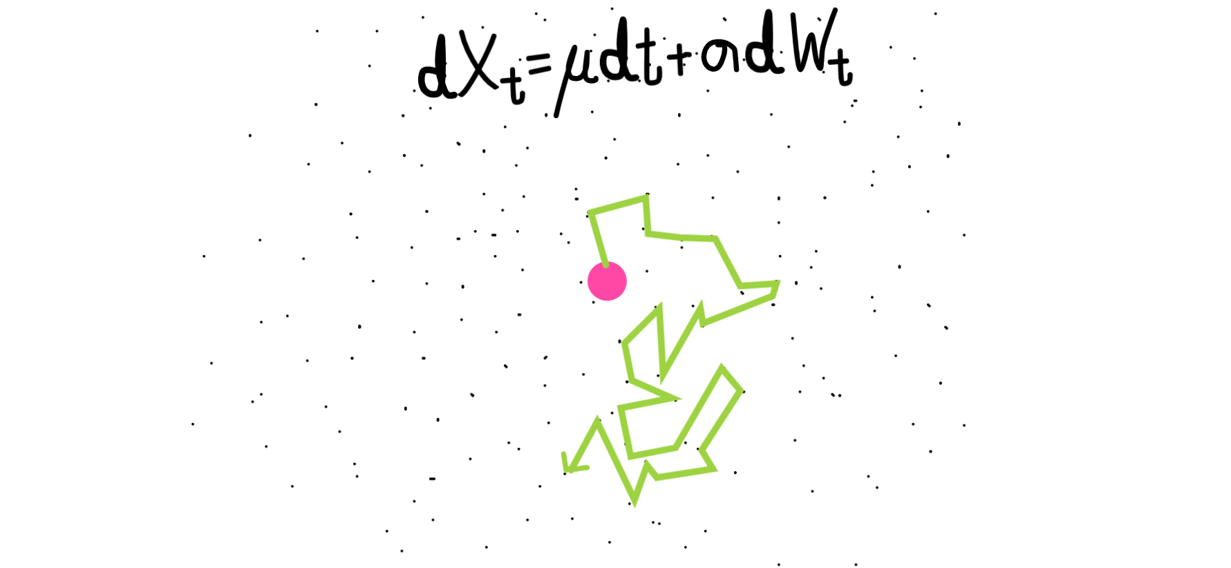
Financial modelers aim to answer this with what we call a continuous-time stochastic model, which is a fancy word to frame our question above. Borrowing from Physics, financial modelers based their modelling of the stock price with what we call a Brownian motion/diffusion – a random process that is closely related to the Normal Distribution. Brownian motion is first used to describe how a pollen grains move randomly after colliding with water molecule, as describe in the figure below:
Black-Scholes Equation & Delta-Hedging
We are going to simplify a lot (really a lot!) of the details in coming up with the B-S equation, but the key idea is to remember what we try to achieve in the binomial option pricing model and generalize the idea into continuous-time. Financial modelers start with the same setup as the binomial tree model: a hedging portfolio. This time, we are instead interested in a dynamic setting, so the delta-hedge (d* in our previous article) is instantaneous and continuous. With some heavy-lifting in stochastic calculus, we arrive at a portfolio that is risk-free, and is able to arrive at the present value through discounting the payoff of the replicating portfolio with the risk-free interest rate.
One of the terms that you’ll often hear people mention is the lognormal distribution. Because of the close relationship of the Brownian motion and the Normal distribution, we are de facto modelling the stock returns (or more precisely, the log-returns) using the normal distribution. As such, the stock price at a after a given period of time will follow a lognormal distribution, which is a skewed and non-zero.
An important thing to note here is on the form of the solution of the option price. While a nice pricing equation does exists for in more vanilla options which are not path-dependent (i.e. you could not exercise the option mid-way through the contract), they don’t exist for exotic products which are path-dependent. In those cases, we’ll have to use a technique called Monte-Carlo Simulation to approximate the price.
You may also be interested in How to Sum and Count Cells by Color in Excel?
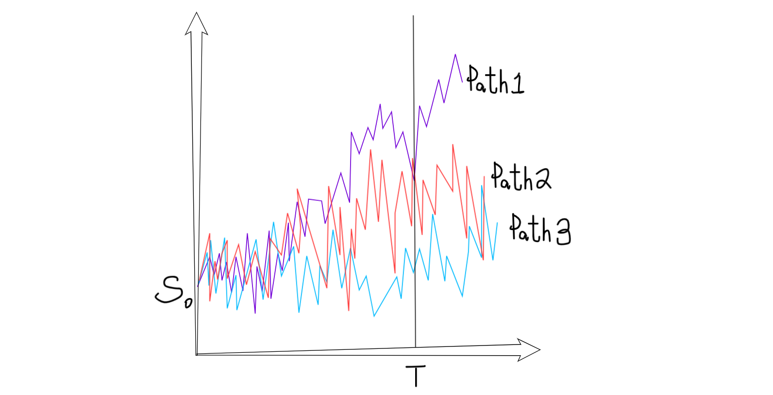
Under Black-Scholes, stock price is assumed to be distributed lognormally.
European Options – With nice equations
Since European options are not path-dependent, we do have nice equations to describe their price under the Black-Scholes model. This is again a result of modelling the stock price under a lognormal distribution (which comes from the Brownian Motion), and therefore we can deduce a general pricing formula for European options. If you are interested in the derivation, you can check it out at the end of this article, but otherwise we’ll take the results as granted and apply it to Excel.
Let’s start from the pricing input:
- S0: Initial stock price
- K: Strike price
- r: Risk-free rate of interest
- σ: Volatility of the stock
- T: Time to maturity
Given the following input, the appropriate (i.e. no-arbitrage) price for a European call option is provided by applying the formula shown below. Don’t be discouraged by the seemingly complicated formula! As usual, let’s give the components a economic interpretation and understanding the concepts behind.
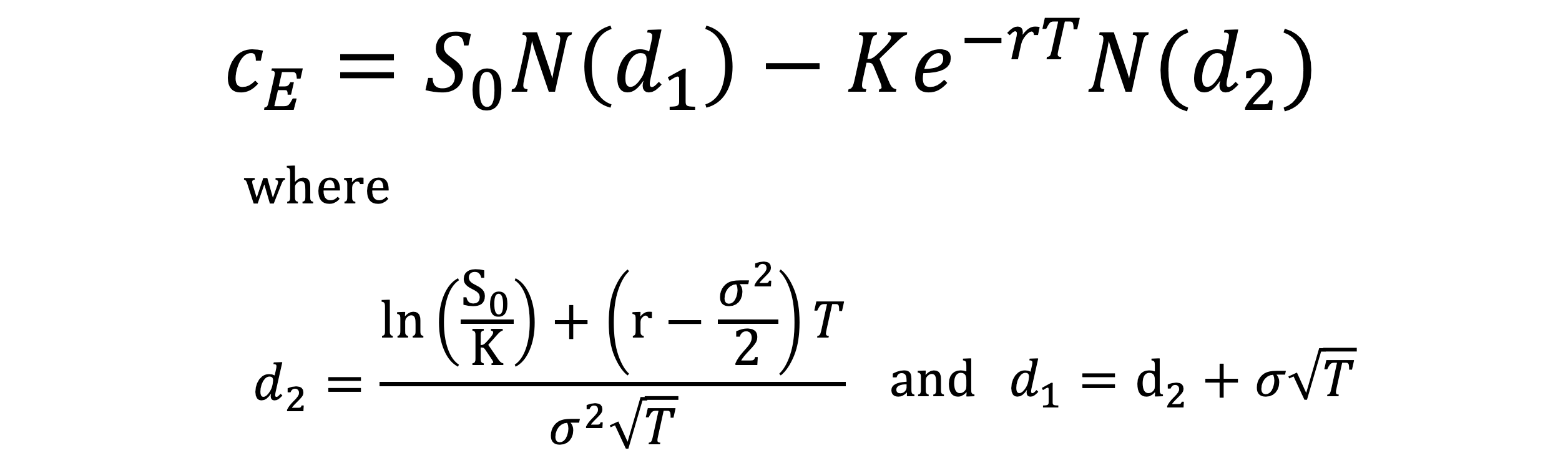
At first glance, you may notice that the formula is in the format similar to the payoff of a call option, which is S – K. The only difference is the N(d1) or the N(d2) that is applied to S and K separately. While the math is complicated, the intuition is:
- S0N(d1) is the conditional expected value of the stock price at maturity, given that the option is in-the-money
- N(d2) is the probability of in-the-moneyness, i.e. the expected value of the price you paid for the stock at maturity is the discounted strike price multiplied by N(d2)
You may also be interested in How To Reverse Concatenate In Excel (3 ways)
European Option in Excel
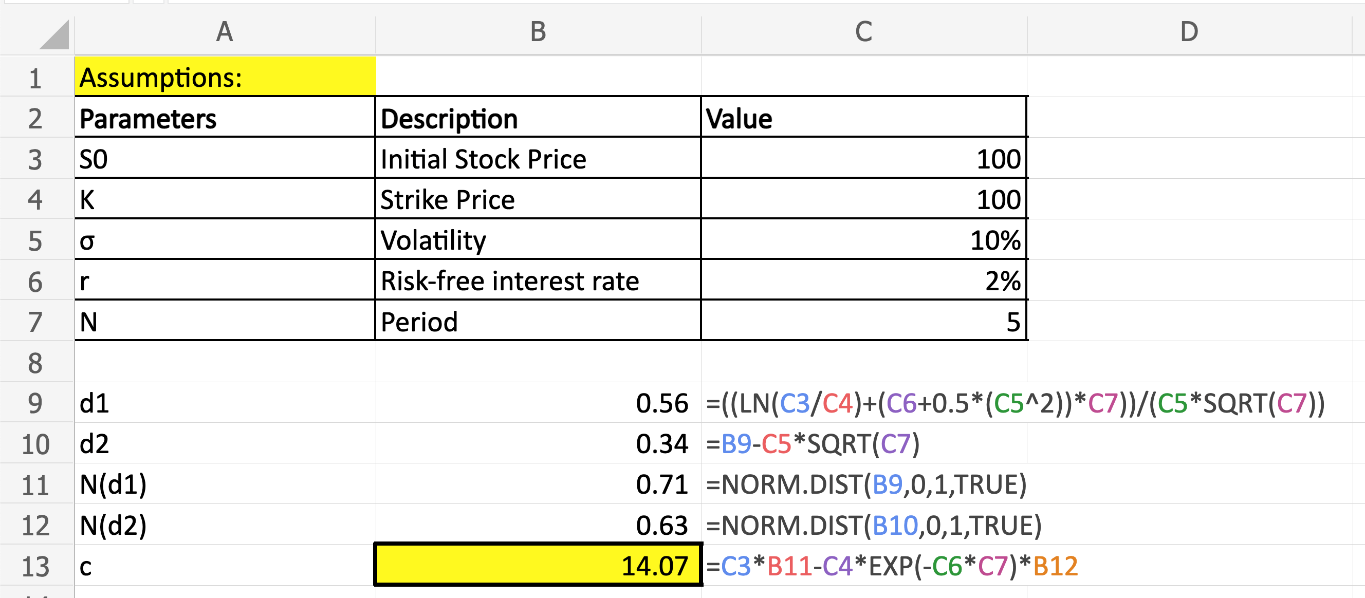
Applying the formula we have in the above, we can easily price any European option as long as we have the 5 inputs available to us! One thing to keep in mind here is on N(d1) and N(d2). Since we are trying compute the cumulative probability function of a standard normal random variable at d1 (or d2), we need to use the Excel functions =NORM.DIST(d1,0,1,TRUE), where 0 and 1 are the mean/standard deviation of the Normal distribution respectively.
Try it out yourself and see if you can get the formula correct in Excel!
What’s Next?
In our next article, we are going to introduce an even more sophisticated and interesting way to price options in Excel – Monte-Carlo Simulation. We’ll start with an example for American option and work our way to learn about VBA as well.
You may also be interested in 2021 New Year Resolution List for Excel
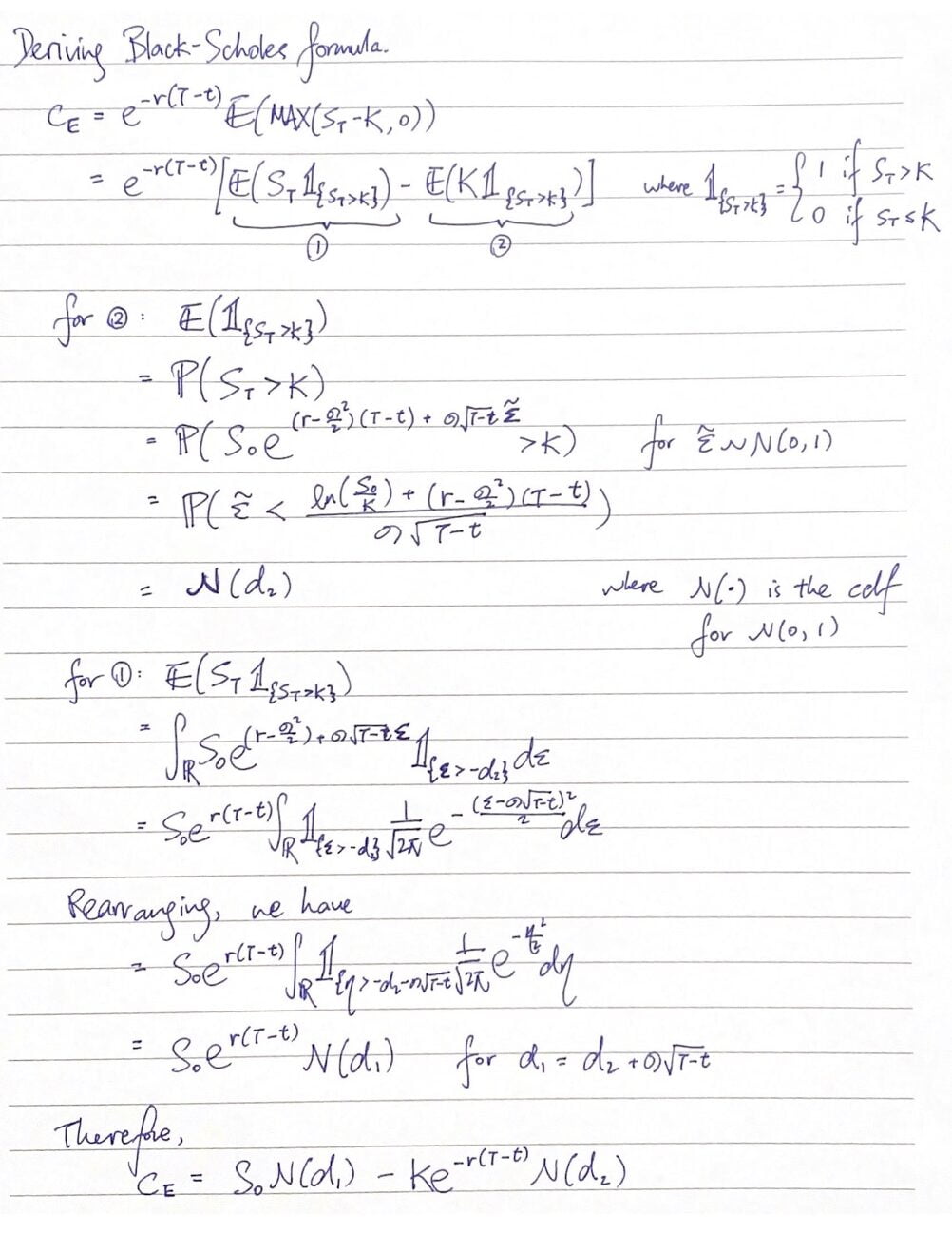
Appendix: Deriving the Black-Scholes formula
This part is for the geeks: we outline a proof to arrive at the Black-Scholes formula for pricing an European call option below.
Hungry for more useful Excel tips like this? Subscribe to our newsletter to make sure you won’t miss out on any of our posts and get exclusive Excel tips!
Black-Scholes Model (European)
Need a European-style Black-Scholes calculator to compute the value of a Put Option or Call Option? Just interested in how the calculation works? Want something just to double check a calculation? Either way, this spreadsheet will help. All of the formulas can be read (and modified if you think that’s necessary).
Quick and simple to use Black-Scholes Calculator. A total of 8 inputs are necessary for this calculation to work.
Black-Scholes Model (European)
System Requirements & Download

To use this Black-Scholes calculator all you have to do is enter the required inputs (in total there are 8). Each red cell is a required input, so if something happens to be zero, a “0” still needs to be input. Within most of the inputs, there are notes, which provide some additional guidance in completing the related input. Below are some of the links that we’ve referenced within the notes. We think these links will be beneficial:
- Market Price – Yahoo Finance
- Risk Free Rate – Federal Reserve
- Volatility – SpreadsheetShoppe.com, we’ve included another file below that has a volatility calculator included. If your looking for a volatility calculator by itself go here.
Enter information into the cells outlined in red. Option Outputs is all formula driven.
Template Summary
- Simple to use
- Easy to understand
- Notes included to help guide input completion
- Inputs and outputs are clearly defined
- No hidden calculations
- No macros
- Straight forward
Due to the amount of judgement associated with determining the correct inputs, this site does not offer any guidance in that area, the suggestions provided are just that, suggestions. As always, it is up to you to understand each input and to select the inputs necessary.
Once the inputs are entered, both the call option and the put option are calculated. We’ve also shown the formulas for the primary parameters – d1 and d2. The time to expire is shown in Days, Months, and Years. This calculation is based on the Start Date and Expiration Date as well as the number of days in the year. Adjust as necessary. Note, be sure to delete the example information before beginning. Also, all items in the input section are required to be completed; therefore, if an item is zero, enter a “0” in that cell.
For those of you who want this Black-Scholes Model combined with the historical volatility also found on this site we’ve combined them for you in the link below.
On October 27, 2015 / Accounting, Analysis, Audit, Calculator, Downloads, Financial Statements, Portfolio