
Содержание
- Use AND and OR to test a combination of conditions
- Use AND and OR with IF
- Sample data
- Using IF with AND, OR and NOT functions
- Examples
- Using AND, OR and NOT with Conditional Formatting
- Need more help?
- See also
- OR function
- Example
- Examples
- Need more help?
- Using logical functions in Excel: AND, OR, XOR and NOT
- Excel logical functions — overview
- Excel logical functions — facts and figures
- Using the AND function in Excel
- Excel AND function — common uses
- An Excel formula for the BETWEEN condition
- Using the OR function in Excel
- Using the XOR function in Excel
- Using the NOT function in Excel
Use AND and OR to test a combination of conditions
When you need to find data that meets more than one condition, such as units sold between April and January, or units sold by Nancy, you can use the AND and OR functions together. Here’s an example:
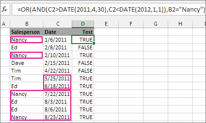
This formula nests the AND function inside the OR function to search for units sold between April 1, 2011 and January 1, 2012, or any units sold by Nancy. You can see it returns True for units sold by Nancy, and also for units sold by Tim and Ed during the dates specified in the formula.
Here’s the formula in a form you can copy and paste. If you want to play with it in a sample workbook, see the end of this article.
Use AND and OR with IF
You can also use AND and OR with the IF function.
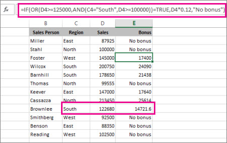
In this example, people don’t earn bonuses until they sell at least $125,000 worth of goods, unless they work in the southern region where the market is smaller. In that case, they qualify for a bonus after $100,000 in sales.
Let’s look a bit deeper. The IF function requires three pieces of data (arguments) to run properly. The first is a logical test, the second is the value you want to see if the test returns True, and the third is the value you want to see if the test returns False. In this example, the OR function and everything nested in it provides the logical test. You can read it as: Look for values greater than or equal to 125,000, unless the value in column C is «South», then look for a value greater than 100,000, and every time both conditions are true, multiply the value by 0.12, the commission amount. Otherwise, display the words «No bonus.»
Sample data
If you want to work with the examples in this article, copy the following table into cell A1 in your own spreadsheet. Be sure to select the whole table, including the heading row.
Источник
Using IF with AND, OR and NOT functions
The IF function allows you to make a logical comparison between a value and what you expect by testing for a condition and returning a result if that condition is True or False.
=IF(Something is True, then do something, otherwise do something else)
But what if you need to test multiple conditions, where let’s say all conditions need to be True or False ( AND), or only one condition needs to be True or False ( OR), or if you want to check if a condition does NOT meet your criteria? All 3 functions can be used on their own, but it’s much more common to see them paired with IF functions.
Use the IF function along with AND, OR and NOT to perform multiple evaluations if conditions are True or False.
IF(AND()) — IF(AND(logical1, [logical2], . ), value_if_true, [value_if_false]))
IF(OR()) — IF(OR(logical1, [logical2], . ), value_if_true, [value_if_false]))
IF(NOT()) — IF(NOT(logical1), value_if_true, [value_if_false]))
The condition you want to test.
The value that you want returned if the result of logical_test is TRUE.
The value that you want returned if the result of logical_test is FALSE.
Here are overviews of how to structure AND, OR and NOT functions individually. When you combine each one of them with an IF statement, they read like this:
AND – =IF(AND(Something is True, Something else is True), Value if True, Value if False)
OR – =IF(OR(Something is True, Something else is True), Value if True, Value if False)
NOT – =IF(NOT(Something is True), Value if True, Value if False)
Examples
Following are examples of some common nested IF(AND()), IF(OR()) and IF(NOT()) statements. The AND and OR functions can support up to 255 individual conditions, but it’s not good practice to use more than a few because complex, nested formulas can get very difficult to build, test and maintain. The NOT function only takes one condition.

Here are the formulas spelled out according to their logic:
=IF(AND(A2>0,B2 0,B4 50),TRUE,FALSE)
IF A6 (25) is NOT greater than 50, then return TRUE, otherwise return FALSE. In this case 25 is not greater than 50, so the formula returns TRUE.
IF A7 (“Blue”) is NOT equal to “Red”, then return TRUE, otherwise return FALSE.
Note that all of the examples have a closing parenthesis after their respective conditions are entered. The remaining True/False arguments are then left as part of the outer IF statement. You can also substitute Text or Numeric values for the TRUE/FALSE values to be returned in the examples.
Here are some examples of using AND, OR and NOT to evaluate dates.

Here are the formulas spelled out according to their logic:
IF A2 is greater than B2, return TRUE, otherwise return FALSE. 03/12/14 is greater than 01/01/14, so the formula returns TRUE.
=IF(AND(A3>B2,A3 B2,A4 B2),TRUE,FALSE)
IF A5 is not greater than B2, then return TRUE, otherwise return FALSE. In this case, A5 is greater than B2, so the formula returns FALSE.

Using AND, OR and NOT with Conditional Formatting
You can also use AND, OR and NOT to set Conditional Formatting criteria with the formula option. When you do this you can omit the IF function and use AND, OR and NOT on their own.
From the Home tab, click Conditional Formatting > New Rule. Next, select the “ Use a formula to determine which cells to format” option, enter your formula and apply the format of your choice.
 Edit Rule dialog showing the Formula method» loading=»lazy»>
Using the earlier Dates example, here is what the formulas would be.

If A2 is greater than B2, format the cell, otherwise do nothing.
=AND(A3>B2,A3 B2,A4 B2)
If A5 is NOT greater than B2, format the cell, otherwise do nothing. In this case A5 is greater than B2, so the result will return FALSE. If you were to change the formula to =NOT(B2>A5) it would return TRUE and the cell would be formatted.
Note: A common error is to enter your formula into Conditional Formatting without the equals sign (=). If you do this you’ll see that the Conditional Formatting dialog will add the equals sign and quotes to the formula — =»OR(A4>B2,A4
Need more help?

See also
You can always ask an expert in the Excel Tech Community or get support in the Answers community.
Источник
OR function
Use the OR function, one of the logical functions, to determine if any conditions in a test are TRUE.
Example
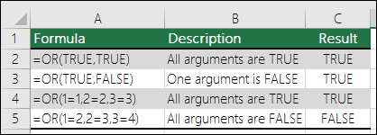
The OR function returns TRUE if any of its arguments evaluate to TRUE, and returns FALSE if all of its arguments evaluate to FALSE.
One common use for the OR function is to expand the usefulness of other functions that perform logical tests. For example, the IF function performs a logical test and then returns one value if the test evaluates to TRUE and another value if the test evaluates to FALSE. By using the OR function as the logical_test argument of the IF function, you can test many different conditions instead of just one.
The OR function syntax has the following arguments:
Required. The first condition that you want to test that can evaluate to either TRUE or FALSE.
Optional. Additional conditions that you want to test that can evaluate to either TRUE or FALSE, up to a maximum of 255 conditions.
The arguments must evaluate to logical values such as TRUE or FALSE, or in arrays or references that contain logical values.
If an array or reference argument contains text or empty cells, those values are ignored.
If the specified range contains no logical values, OR returns the #VALUE! error value.
You can use an OR array formula to see if a value occurs in an array. To enter an array formula, press CTRL+SHIFT+ENTER.
Examples
Here are some general examples of using OR by itself, and in conjunction with IF.
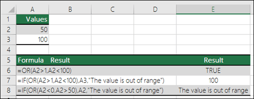
=OR(A2>1,A2 OR less than 100, otherwise it displays FALSE.
=IF(OR(A2>1,A2 OR less than 100, otherwise it displays the message «The value is out of range».
=IF(OR(A2 50),A2,»The value is out of range»)
Displays the value in cell A2 if it’s less than 0 OR greater than 50, otherwise it displays a message.
Sales Commission Calculation
Here is a fairly common scenario where we need to calculate if sales people qualify for a commission using IF and OR.
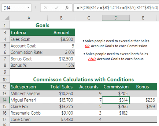
=IF(OR(B14>=$B$4,C14>=$B$5),B14*$B$6,0) — IF Total Sales are greater than or equal to (>=) the Sales Goal, OR Accounts are greater than or equal to (>=) the Account Goal, then multiply Total Sales by the Commission %, otherwise return 0.
Need more help?
You can always ask an expert in the Excel Tech Community or get support in the Answers community.
Источник
Using logical functions in Excel: AND, OR, XOR and NOT
 by Svetlana Cheusheva, updated on October 7, 2022
The tutorial explains the essence of Excel logical functions AND, OR, XOR and NOT and provides formula examples that demonstrate their common and inventive uses.
Last week we tapped into the insight of Excel logical operators that are used to compare data in different cells. Today, you will see how to extend the use of logical operators and construct more elaborate tests to perform more complex calculations. Excel logical functions such as AND, OR, XOR and NOT will help you in doing this.
Excel logical functions — overview
Microsoft Excel provides 4 logical functions to work with the logical values. The functions are AND, OR, XOR and NOT. You use these functions when you want to carry out more than one comparison in your formula or test multiple conditions instead of just one. As well as logical operators, Excel logical functions return either TRUE or FALSE when their arguments are evaluated.
The following table provides a short summary of what each logical function does to help you choose the right formula for a specific task.
| Function | Description | Formula Example | Formula Description |
| AND | Returns TRUE if all of the arguments evaluate to TRUE. | =AND(A2>=10, B2 | The formula returns TRUE if a value in cell A2 is greater than or equal to 10, and a value in B2 is less than 5, FALSE otherwise. |
| OR | Returns TRUE if any argument evaluates to TRUE. | =OR(A2>=10, B2 | The formula returns TRUE if A2 is greater than or equal to 10 or B2 is less than 5, or both conditions are met. If neither of the conditions it met, the formula returns FALSE. |
| XOR | Returns a logical Exclusive Or of all arguments. | =XOR(A2>=10, B2 | The formula returns TRUE if either A2 is greater than or equal to 10 or B2 is less than 5. If neither of the conditions is met or both conditions are met, the formula returns FALSE. |
| NOT | Returns the reversed logical value of its argument. I.e. If the argument is FALSE, then TRUE is returned and vice versa. | =NOT(A2>=10) | The formula returns FALSE if a value in cell A1 is greater than or equal to 10; TRUE otherwise. |
In additions to the four logical functions outlined above, Microsoft Excel provides 3 «conditional» functions — IF, IFERROR and IFNA.
Excel logical functions — facts and figures
- In arguments of the logical functions, you can use cell references, numeric and text values, Boolean values, comparison operators, and other Excel functions. However, all arguments must evaluate to the Boolean values of TRUE or FALSE, or references or arrays containing logical values.
- If an argument of a logical function contains any empty cells, such values are ignored. If all of the arguments are empty cells, the formula returns #VALUE! error.
- If an argument of a logical function contains numbers, then zero evaluates to FALSE, and all other numbers including negative numbers evaluate to TRUE. For example, if cells A1:A5 contain numbers, the formula =AND(A1:A5) will return TRUE if none of the cells contains 0, FALSE otherwise.
- A logical function returns the #VALUE! error if none of the arguments evaluate to logical values.
- A logical function returns the #NAME? error if you’ve misspell the function’s name or attempted to use the function in an earlier Excel version that does not support it. For example, the XOR function can be used in Excel 2016 and 2013 only.
- In Excel 2007 and higher, you can include up to 255 arguments in a logical function, provided that the total length of the formula does not exceed 8,192 characters. In Excel 2003 and lower, you can supply up to 30 arguments and the total length of your formula shall not exceed 1,024 characters.
Using the AND function in Excel
The AND function is the most popular member of the logic functions family. It comes in handy when you have to test several conditions and make sure that all of them are met. Technically, the AND function tests the conditions you specify and returns TRUE if all of the conditions evaluate to TRUE, FALSE otherwise.
The syntax for the Excel AND function is as follows:
Where logical is the condition you want to test that can evaluate to either TRUE or FALSE. The first condition (logical1) is required, subsequent conditions are optional.
And now, let’s look at some formula examples that demonstrate how to use the AND functions in Excel formulas.
| Formula | Description |
| =AND(A2=»Bananas», B2>C2) | Returns TRUE if A2 contains «Bananas» and B2 is greater than C2, FALSE otherwise. |
| =AND(B2>20, B2=C2) | Returns TRUE if B2 is greater than 20 and B2 is equal to C2, FALSE otherwise. |
| =AND(A2=»Bananas», B2>=30, B2>C2) | Returns TRUE if A2 contains «Bananas», B2 is greater than or equal to 30 and B2 is greater than C2, FALSE otherwise. |

Excel AND function — common uses
By itself, the Excel AND function is not very exciting and has narrow usefulness. But in combination with other Excel functions, AND can significantly extend the capabilities of your worksheets.
One of the most common uses of the Excel AND function is found in the logical_test argument of the IF function to test several conditions instead of just one. For example, you can nest any of the AND functions above inside the IF function and get a result similar to this:
=IF(AND(A2=»Bananas», B2>C2), «Good», «Bad») 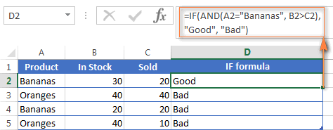
For more IF / AND formula examples, please check out his tutorial: Excel IF function with multiple AND conditions.
An Excel formula for the BETWEEN condition
If you need to create a between formula in Excel that picks all values between the given two values, a common approach is to use the IF function with AND in the logical test.
For example, you have 3 values in columns A, B and C and you want to know if a value in column A falls between B and C values. To make such a formula, all it takes is the IF function with nested AND and a couple of comparison operators:
Formula to check if X is between Y and Z, inclusive:
Formula to check if X is between Y and Z, not inclusive:
=IF(AND(A2>B2, A2 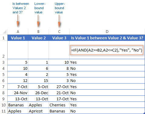
As demonstrated in the screenshot above, the formula works perfectly for all data types — numbers, dates and text values. When comparing text values, the formula checks them character-by-character in the alphabetic order. For example, it states that Apples in not between Apricot and Bananas because the second «p» in Apples comes before «r» in Apricot. Please see Using Excel comparison operators with text values for more details.
As you see, the IF /AND formula is simple, fast and almost universal. I say «almost» because it does not cover one scenario. The above formula implies that a value in column B is smaller than in column C, i.e. column B always contains the lower bound value and C — the upper bound value. This is the reason why the formula returns «No» for row 6, where A6 has 12, B6 — 15 and C6 — 3 as well as for row 8 where A8 is 24-Nov, B8 is 26-Dec and C8 is 21-Oct.
But what if you want your between formula to work correctly regardless of where the lower-bound and upper-bound values reside? In this case, use the Excel MEDIAN function that returns the median of the given numbers (i.e. the number in the middle of a set of numbers).
So, if you replace AND in the logical test of the IF function with MEDIAN, the formula will go like:
And you will get the following results: 
As you see, the MEDIAN function works perfectly for numbers and dates, but returns the #NUM! error for text values. Alas, no one is perfect : )
If you want a perfect Between formula that works for text values as well as for numbers and dates, then you will have to construct a more complex logical text using the AND / OR functions, like this:
=IF(OR(AND(A2>B2, A2 C2)), «Yes», «No») 
Using the OR function in Excel
As well as AND, the Excel OR function is a basic logical function that is used to compare two values or statements. The difference is that the OR function returns TRUE if at least one if the arguments evaluates to TRUE, and returns FALSE if all arguments are FALSE. The OR function is available in all versions of Excel 2016 — 2000.
The syntax of the Excel OR function is very similar to AND:
Where logical is something you want to test that can be either TRUE or FALSE. The first logical is required, additional conditions (up to 255 in modern Excel versions) are optional.
And now, let’s write down a few formulas for you to get a feel how the OR function in Excel works.
| Formula | Description |
| =OR(A2=»Bananas», A2=»Oranges») | Returns TRUE if A2 contains «Bananas» or «Oranges», FALSE otherwise. |
| =OR(B2>=40, C2>=20) | Returns TRUE if B2 is greater than or equal to 40 or C2 is greater than or equal to 20, FALSE otherwise. |
| =OR(B2=» «, C2=»») | Returns TRUE if either B2 or C2 is blank or both, FALSE otherwise. |

As well as Excel AND function, OR is widely used to expand the usefulness of other Excel functions that perform logical tests, e.g. the IF function. Here are just a couple of examples:
IF function with nested OR
=IF(OR(B2>30, C2>20), «Good», «Bad»)
The formula returns «Good» if a number in cell B3 is greater than 30 or the number in C2 is greater than 20, «Bad» otherwise.
Excel AND / OR functions in one formula
Naturally, nothing prevents you from using both functions, AND & OR, in a single formula if your business logic requires this. There can be infinite variations of such formulas that boil down to the following basic patterns:
=AND(OR(Cond1, Cond2), Cond3)
=AND(OR(Cond1, Cond2), OR(Cond3, Cond4)
=OR(AND(Cond1, Cond2), Cond3)
For example, if you wanted to know what consignments of bananas and oranges are sold out, i.e. «In stock» number (column B) is equal to the «Sold» number (column C), the following OR/AND formula could quickly show this to you:
=OR(AND(A2=»bananas», B2=C2), AND(A2=»oranges», B2=C2)) 
OR function in Excel conditional formatting
The rule with the above OR formula highlights rows that contain an empty cell either in column B or C, or in both. 
For more information about conditional formatting formulas, please see the following articles:
Using the XOR function in Excel
In Excel 2013, Microsoft introduced the XOR function, which is a logical Exclusive OR function. This term is definitely familiar to those of you who have some knowledge of any programming language or computer science in general. For those who don’t, the concept of ‘Exclusive Or’ may be a bit difficult to grasp at first, but hopefully the below explanation illustrated with formula examples will help.
The syntax of the XOR function is identical to OR’s :
The first logical statement (Logical 1) is required, additional logical values are optional. You can test up to 254 conditions in one formula, and these can be logical values, arrays, or references that evaluate to either TRUE or FALSE.
In the simplest version, an XOR formula contains just 2 logical statements and returns:
- TRUE if either argument evaluates to TRUE.
- FALSE if both arguments are TRUE or neither is TRUE.
This might be easier to understand from the formula examples:
| Formula | Result | Description |
| =XOR(1>0, 2 | TRUE | Returns TRUE because the 1st argument is TRUE and the 2 nd argument is FALSE. |
| =XOR(1 | FALSE | Returns FALSE because both arguments are FALSE. |
| =XOR(1>0, 2>1) | FALSE | Returns FALSE because both arguments are TRUE. |
When more logical statements are added, the XOR function in Excel results in:
- TRUE if an odd number of the arguments evaluate to TRUE;
- FALSE if is the total number of TRUE statements is even, or if all statements are FALSE.
The screenshot below illustrates the point: 
If you are not sure how the Excel XOR function can be applied to a real-life scenario, consider the following example. Suppose you have a table of contestants and their results for the first 2 games. You want to know which of the payers shall play the 3 rd game based on the following conditions:
- Contestants who won Game 1 and Game 2 advance to the next round automatically and don’t have to play Game 3.
- Contestants who lost both first games are knocked out and don’t play Game 3 either.
- Contestants who won either Game 1 or Game 2 shall play Game 3 to determine who goes into the next round and who doesn’t.
A simple XOR formula works exactly as we want:
=XOR(B2=»Won», C2=»Won») 
And if you nest this XOR function into the logical test of the IF formula, you will get even more sensible results:
=IF(XOR(B2=»Won», C2=»Won»), «Yes», «No») 
Using the NOT function in Excel
The NOT function is one of the simplest Excel functions in terms of syntax:
You use the NOT function in Excel to reverse a value of its argument. In other words, if logical evaluates to FALSE, the NOT function returns TRUE and vice versa. For example, both of the below formulas return FALSE:
Why would one want to get such ridiculous results? In some cases, you might be more interested to know when a certain condition isn’t met than when it is. For example, when reviewing a list of attire, you may want to exclude some color that does not suit you. I’m not particularly fond of black, so I go ahead with this formula:
=NOT(C2=»black») 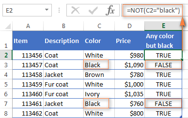
As usual, in Microsoft Excel there is more than one way to do something, and you can achieve the same result by using the Not equal to operator: =C2<>«black».
If you want to test several conditions in a single formula, you can use NOT in conjunctions with the AND or OR function. For example, if you wanted to exclude black and white colors, the formula would go like:
And if you’d rather not have a black coat, while a black jacket or a back fur coat may be considered, you should use NOT in combination with the Excel AND function:
Another common use of the NOT function in Excel is to reverse the behavior of some other function. For instance, you can combine NOT and ISBLANK functions to create the ISNOTBLANK formula that Microsoft Excel lacks.
As you know, the formula =ISBLANK(A2) returns TRUE of if the cell A2 is blank. The NOT function can reverse this result to FALSE: =NOT(ISBLANK(A2))
And then, you can take a step further and create a nested IF statement with the NOT / ISBLANK functions for a real-life task:
=IF(NOT(ISBLANK(C2)), C2*0.15, «No bonus :(«) ![]()
Translated into plain English, the formula tells Excel to do the following. If the cell C2 is not empty, multiply the number in C2 by 0.15, which gives the 15% bonus to each salesman who has made any extra sales. If C2 is blank, the text «No bonus :(» appears.
In essence, this is how you use the logical functions in Excel. Of course, these examples have only scratched the surface of AND, OR, XOR and NOT capabilities. Knowing the basics, you can now extend your knowledge by tackling your real tasks and writing smart elaborate formulas for your worksheets.
Источник
INTRODUCTION
OR function comes under the LOGICAL FUNCTIONS category in Excel.
OR function is very important and is going to be used a lot which makes it one of the very important functions in excel.
It simply behaves like the binary OR.
It checks if ANY OF THE CONDITIONS are TRUE OR NOT.
IT returns TRUE if ANY OF THE CONDITIONS ARE TRUE and false , if ALL of the conditions is FALSE.
PURPOSE OF OR IN EXCEL
OR FUNCTION RETURNS TRUE IF ANY OF THE CONDITIONS ARE TRUE AND FALSE IF ALL OF THE GIVEN CONDITIONS ARE FALSE.
PREREQUISITES TO LEARN OR
THERE ARE A FEW PREREQUISITES WHICH WILL ENABLE YOU TO UNDERSTAND THIS FUNCTION IN A BETTER WAY.
- Some information about the BINARY MATHEMATICS is an advantage for the use of such formulas.
- Basic understanding of how to use a formula or function.
- Basic understanding of rows and columns in Excel.
- Of course, Excel software.
Helpful links for the prerequisites mentioned above
What Excel does? How to use formula in Excel?
SYNTAX: OR FUNCTION
The Syntax for the function is
=OR(CONDITION 1, CONDITION 2, CONDITION 3, …… SO ON)
CONDITION1 Any condition (e.g. if any cell>12)
CONDITION2 Any condition (if any cell <45)
Atleast TWO CONDITIONS are needed. At the most, any number of conditions can be used.
EXAMPLE:OR FUNCTION IN EXCEL
DATA SAMPLE
Suppose we have a cell which contains a number. Suppose we are trying to make a group of the people with ages <20 and greater than 50. For this case, we can use OR function as we have to select the person when either of the conditions is true.
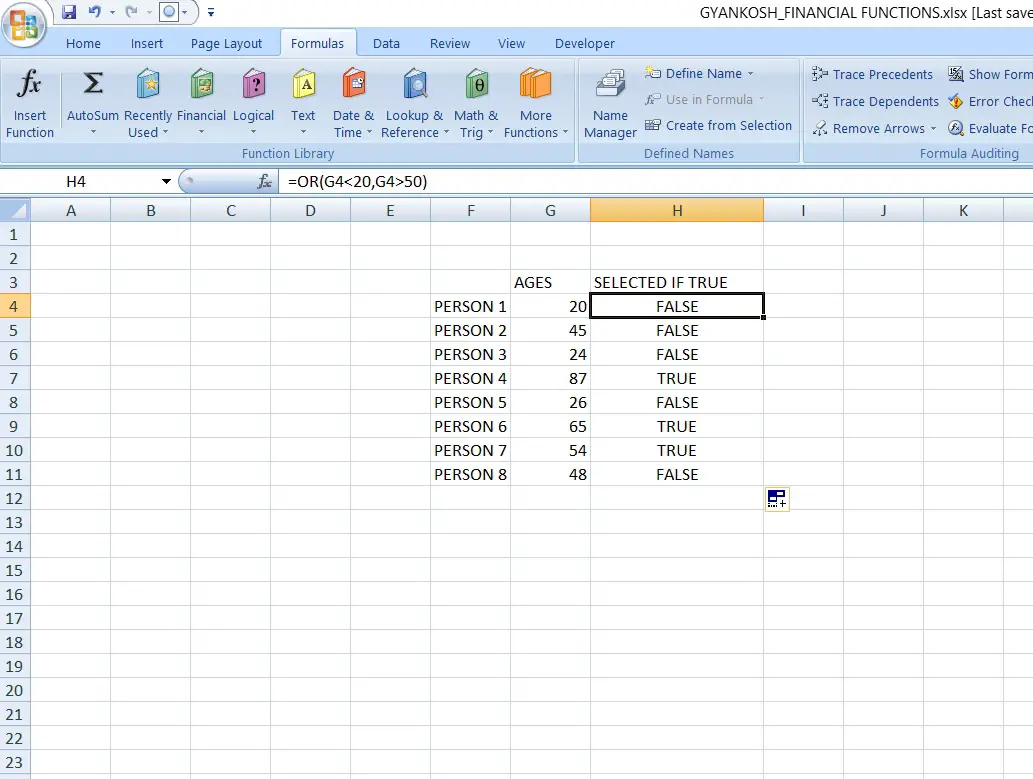
STEPS TO USE OR
The example has 8 persons with ages given in the next column.
We are checking if the age is fulfilling the requirement for the selection which is, the age needs to be less than 20 or greater than 50
The formula is used as
=OR(G4<20,G4>50)
for the PERSON 1 and goes like this. for person 8 it is
=OR(G11<20,G11>50)
The cell number is the cell which contains the age of a particular person.
KNOWLEDGE BYTES
BINARY OR
BINARY MATHEMATICS have just two number-0 and 1.Its just like the DECIMAL SYSTEM which we use in day to day life which has ten numbers 0 to 9.So OR is known as the BINARY ADDITION. As we can understand easily that0+0=01+0=10+1=11+1=1where 1 is TRUE and 0 is false.Same goes in this function. When any of the conditions are true, we get TRUE result.
DIFFERENCES: AND vs OR
AND is binary multiplication whereas OR is binary addition.AND needs all the conditions true to give TRUE as result.OR needs any of the condition true to give TRUE as result.
Excel for Microsoft 365 Excel for Microsoft 365 for Mac Excel for the web Excel 2021 Excel 2021 for Mac Excel 2019 Excel 2019 for Mac Excel 2016 Excel 2016 for Mac Excel 2013 Excel 2010 Excel 2007 Excel for Mac 2011 Excel Starter 2010 More…Less
To get detailed information about a function, click its name in the first column.
Note: Version markers indicate the version of Excel a function was introduced. These functions aren’t available in earlier versions. For example, a version marker of 2013 indicates that this function is available in Excel 2013 and all later versions.
|
Function |
Description |
|---|---|
|
AND function |
Returns TRUE if all of its arguments are TRUE |
|
BYCOL function |
Applies a LAMBDA to each column and returns an array of the results |
|
BYROW function |
Applies a LAMBDA to each row and returns an array of the results |
|
FALSE function |
Returns the logical value FALSE |
|
IF function |
Specifies a logical test to perform |
|
IFERROR function |
Returns a value you specify if a formula evaluates to an error; otherwise, returns the result of the formula |
|
IFNA function |
Returns the value you specify if the expression resolves to #N/A, otherwise returns the result of the expression |
|
IFS function |
Checks whether one or more conditions are met and returns a value that corresponds to the first TRUE condition. |
|
LAMBDA function |
Create custom, reusable functions and call them by a friendly name |
|
LET function |
Assigns names to calculation results |
|
MAKEARRAY function |
Returns a calculated array of a specified row and column size, by applying a LAMBDA |
|
MAP function |
Returns an array formed by mapping each value in the array(s) to a new value by applying a LAMBDA to create a new value |
|
NOT function |
Reverses the logic of its argument |
|
OR function |
Returns TRUE if any argument is TRUE |
|
REDUCE function |
Reduces an array to an accumulated value by applying a LAMBDA to each value and returning the total value in the accumulator |
|
SCAN function |
Scans an array by applying a LAMBDA to each value and returns an array that has each intermediate value |
|
SWITCH function |
Evaluates an expression against a list of values and returns the result corresponding to the first matching value. If there is no match, an optional default value may be returned. |
|
TRUE function |
Returns the logical value TRUE |
|
XOR function |
Returns a logical exclusive OR of all arguments |


Important: The calculated results of formulas and some Excel worksheet functions may differ slightly between a Windows PC using x86 or x86-64 architecture and a Windows RT PC using ARM architecture. Learn more about the differences.
See Also
Excel functions (by category)
Excel functions (alphabetical)
Need more help?
Want more options?
Explore subscription benefits, browse training courses, learn how to secure your device, and more.
Communities help you ask and answer questions, give feedback, and hear from experts with rich knowledge.
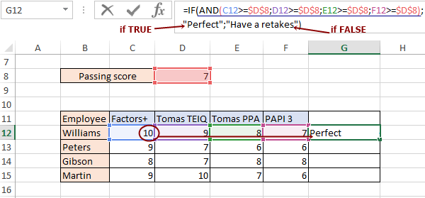
The AND function is a logical function. It allows you to define the conditions that it checks for the result TRUE if all conditions are met (FALSE if at least one condition is not met). The OR function is also a logical function, which, unlike «AND», determines only one of the available conditions for the result TRUE (FALSE — if all the conditions being checked are not met).
Boolean functions in Excel practical work
Concept of AND OR, the syntax for both functions is as follows:
Boolean value 1 is a required argument, and the number of subsequent ones depends on the task. Now let’s see how these functions work. We have a form about the results of tests that were conducted among employees and the passing score is indicated. We need to find out which of the employees coped with all the tests and who did not. To do this, we indicate in the formula that we will check AND the first test, AND the second, AND the third, AND the fourth, each must be at least 7 (cell D8):
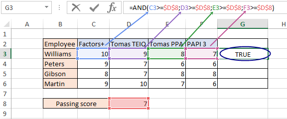
As a result, in cell G3 we got the result TRUE, since all conditions are met. Be sure to use absolute references and copy the formula to the end of the column. Now we have the result for all employees:
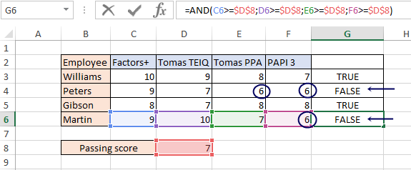
Since we have the value 6 in cells E4, F4 and F6, the condition was not met and the result FALSE was returned and we found out which of the employees failed at least one test, and who coped with all and can continue to work. But the words «TRUE» or «FALSE» do not quite correctly reflect the meaning of the results. Therefore, we add two more expressions to the function — «Perfect» will be used if TRUE, and «Have a retakes» will be used if FALSE. The IF function will help us with this, in which we will embed the AND function:
Copy the function to the end of the column and get the finished table:
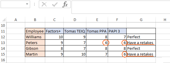
Opposite the cells, the value of which is less than 7, we got the result “Have a retakes”.
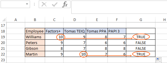
Now let’s look at how the OR function works. We still have the same tests and employees, but now we need to check if we have an excellent one in at least one test. That is, is there a value of 10 among the values of cells C19, D19, E19, F19:
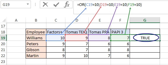
We got the value TRUE because the value of cell C19 is 10. Now we copy our formula to the end and get the result for the rest of the employees:
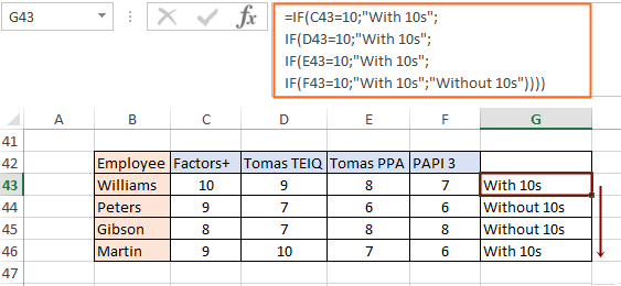
For more correct informativeness, we will replace the result “TRUE” with the phrase “With 10s”, and the result “FALSE” with the phrase “Without 10s”. To do this, we also use the IF function, in which we put the OR formula:
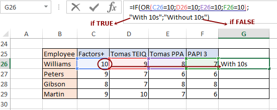
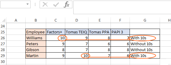
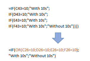
In cell C26, we have the value 10, so the formula returned the value if TRUE — «With 10s.» Copy the formula to the end of the column and get the finished table:
Using AND OR functions instead of nested IF functions
Sometimes, using AND/OR functions, nested IF functions can be avoided. Nested functions are a good tool, but they become unwieldy when new conditions are added. For example, our task “Determine which employees completed all the tests and who needs to improve them” can be executed with nested IF functions:
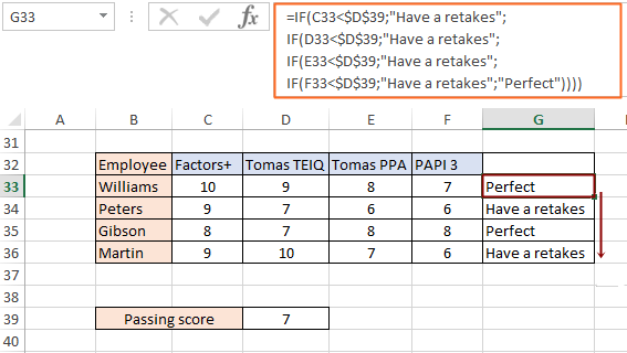
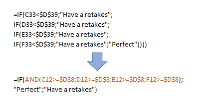
In cell G33, we built a nested function and copied it to the end of the column. We got the same results as using IF + AND, however, the formula itself is very long, it will be easy to get confused in it if we need to add new conditions. In addition, working with it will take more time, although they perform the task correctly and in the same way. Therefore, it is better to give preference to the IF function using the AND function:
The second example, where we used IF+OR to find which employee got the highest score, we can also consider using nested IF functions:
We got the same results. However, if we compare the formulas of these two examples, the IF+OR function is much shorter and more accurate, especially when new conditions are added:
How combinations IF+AND+OR, IF+OR+AND work
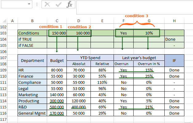
Sometimes AND, OR, IF functions are used simultaneously. Before delving into some of these examples, let’s reinforce the use of formulas we already know. We have budget information for various departments. We want to check if the budget amount of a certain department exceeds the value of 100,000 AND if the absolute expenditures since the beginning of the year exceed the value of 50,000. If these two conditions are met, we will indicate the word “Done”, and if not, the sign “-”. Specify absolute references for cells with conditions, otherwise when copying the formula, the values will also be omitted:
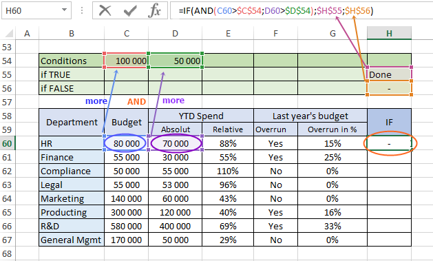
We got a «-» result because only one condition was met — 70,000 is greater than 50,000, but 80,000 is not greater than 100,000. Let’s copy our formula to the end of the column and determine which departments meet the conditions:
In this example, we have specified certain conditions that must be met at the same time. Now let’s look at an example where we expand the functionality of the formula by adding the OR function. Let’s leave the two conditions known to us from the previous example — the budget exceeds 100,000, the absolute expenses exceed 50,000 and add new conditions through the OR function: was there a budget overrun last year OR was the budget overrun by more than 20%. Now we have 4 conditions, but only if three of them are true — we will get the value «Done»:

We used a combination of IF + AND + OR functions. Let’s copy the formula to the end of the column and see the departments whose data match the conditions we specified:
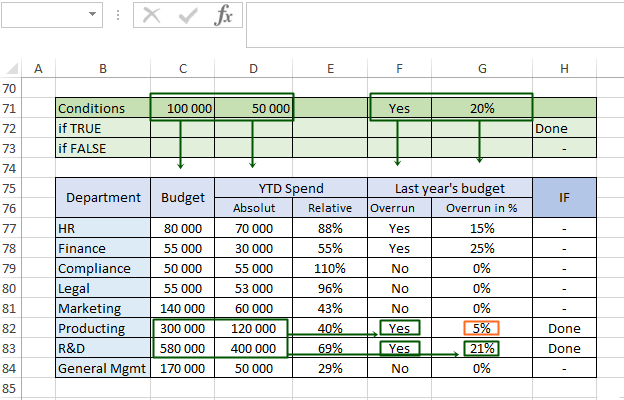
The production department and R&D met our conditions because the budget exceeds 100,000 AND the absolute expenses exceed 50,000, in addition, the R&D department has an over budget of more than 20%, and the production department has an over budget, but less than 20% — this is enough to comply with our terms and conditions.
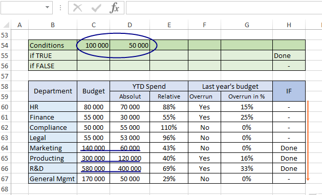
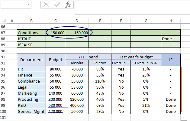
Now let’s search for departments that will match one of the given conditions. The principle of operation is the same as in the example with the fulfillment of the conditions “Budget is more than 100,000 AND absolute expenses are more than 50,000”, but this time we will change the requirements — we need departments that fulfill AT LEAST one requirement: budget is more than 150,000 or absolute expenses more than 160,000. The IF + OR functions will help us with this:
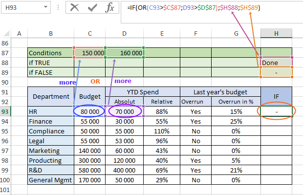
We copy the formula and see that the status «Done» was received by those departments that satisfied one of the requirements:
Finally, consider the last combination of IF + OR + AND functions. In this case, we need to add the last AND function as the third condition of the OR function. For the AND function, we will indicate two requirements — the presence of an excess of the budget, an excess of more than 10%:
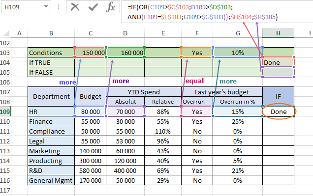
This combination matches AT LEAST one of the three requirements:
- Budget over 150,000.
- Absolute expenses are more than 160,000.
- The presence of an excess of the last year’s budget, the excess indicator is more than 10%.
Copy the formula to the end of the table and check which departments have met our requirements:
 Download logical functions AND OR in Excel with examples
This is how logical functions work in Excel using additional formulas to solve multi-tasking problems.
Excel AND + OR Functions: Full Guide (with IF Formulas)
The AND and OR functions returns True or False if certain conditions are met.
Combined with other functions, like IF, that enables multiple criteria logic in your formulas.
In this guide, I’ll walk you through all of this, step-by-step 👍🏼
If you want to tag along, download the sample workbook here.
We use the data in the following table to learn how to apply OR and AND function with the IF function in excel.

The OR function
The OR function is one of the most important logical functions in excel 😯
The OR function in Excel returns True if at least one of the criteria evaluates to true.
If all the arguments evaluate as False, then the OR function returns False.
The syntax of the OR function in Excel is OR(logical1, [logical2], …).
Assume that employees are eligible for an incentive if they achieve a value or volume target of 75% or more 🏆
Let’s try OR function for the above example.
- Enter an equal sign and select the OR function.
You will see below in the formula bar.
=OR(

- Supply the first logical value to evaluate as the first argument.
You can write logical values to test using logical operators.
In this case, we want to first test, whether the value target achievement is greater than or equal to 75%.
So, we can give the cell reference and write the condition >=75%.
Now the formula is,
=OR(B3>=75%

- Enter a comma and enter the 2nd logical value for the logical test.
Then, we enter the logical value for the volume target.
Now, the updated formula is;
=OR(B3>7=75%,C3>=75%

- Close the parentheses and press enter.
The below Excel formula evaluates arguments.
=OR(B3>7=75%,C3>=75%)
Then returns true if at least one of the value or volume target achievements is greater than or equal to 75%. If both value and volume target achievements are below 75%, the OR function returns False.

Pro Tip:
Now you have learned, the OR function returns True even when more than one condition evaluates to “True”.
Do you think you have to combine the OR function with the NOT function?
No. Excel has a simple solution 😜
You have to use the XOR function.
Apply the below XOR formula to the above example and see how the results are changing.
=XOR(B3>7=75%,C3>=75%)

You can see that Mary’s result is “False” as her achievements are not satisfying the one and only condition.
OR function IF formula example
Isn’t it boring to see only “True or false” values? 🥱
Don’t you like to get something other than True or False values? 👍
You just need to combine the OR function with the IF function in Excel.
Let’s say, we want the function to return “Eligible” if at least one of the value or volume target achievements is greater than or equal to 75%.
Also, return “Not eligible”, if both value and volume target achievements are less than 75%.
- Enter the equal sign and select the IF function.
Now, the formula bar will show;

- Enter the OR function that we have learned in the previous section.
The updated formula should be like this.
=IF(OR(B3>=75%,C3>=75%)

- Enter the specific value you want the function to return when the result of the logical test is True.
In this case, we want to get “Eligible”.
So, we enter the word eligible within quotes.
Now, the formula is;
=IF(OR(B3>=75%,C3>=75%),”Eligible”

If you want to enter text values for the arguments, you have to enter them within quotes. However, you don’t need to enter True or false values within quotes. Excel automatically evaluates arguments provided with true or false values.
- Enter the specific value you want the function to return when the result of the logical test is False.
In this case, we want to get “Not Eligible”.
Now, the updated formula is;
=IF(OR(B3>=75%,C3>=75%),”Eligible”,”Not Eligible”

- Close the parentheses and press “Enter”.

The AND function
AND function is another important logical function in excel.
This function returns true all of the multiple criteria are true.
Otherwise, the AND function returns False.
The syntax of the AND function in Excel is AND(logical1, [logical2], …).
Say that employees are entitled to an incentive if they achieve more than or equal to 75% for both the value target and volume target.
Let’s try AND function for the above example.
- Enter an equal sign and select the AND function.
You will see below in the formula bar.
=AND(

- Enter all logical values to test using logical operators.
So, you can enter the following formula.
=AND(B3>=75%,C3>=75%

- Close the parentheses and press “Enter”.

You can see that the AND function returns true only when both the value and volume target achievements exceed or are equal to 75% 🥳
However, there is limited usage of AND function if we do not combine it with other functions in Excel 🤔
Let’s see an example with a combination of the IF function and AND function.
AND function IF formula example
Let’s say, we want the function to return “Eligible”, only when both value and volume target achievements are more than or equal to 75%.
Otherwise, we want to get “Not eligible”
- Enter the equals sign and select the IF function.
Now, the formula bar will show;

- Enter the AND function that we have learned in the previous section.
The updated formula should be like this.
=IF(AND(B3>=75%,C3>=75%)

- Enter the specific value you want the function to return when the result of the logical test is True.
In this case, we want to get “Eligible”.
So, we enter the word eligible within quotes.
Now, the formula is;
=IF(AND(B3>=75%,C3>=75%),”Eligible”

- Enter the specific value you want the function to return when the result of the logical test is False.
In this case, we want to get “Not Eligible”.
Now, the updated formula is;
=IF(AND(B3>=75%,C3>=75%),”Eligible”,”Not Eligible”

- Close the parentheses and press “Enter”.

You can see that we get “Eligible” only when all of the multiple conditions are True. Otherwise, functions will return false 😍
Any empty cells in a logical function’s argument are ignored.

That’s it – Now what?
Well done 👏🏻
Now you know how to use the OR and AND functions in Excel.
Using the above examples, you have learned that OR and AND functions are more powerful when we combine them with other Excel functions 💪🏻
To learn more about other important functions such as IF, SUMIF, and VLOOKUP functions, all you need to do is enroll in my free 30-minute online Excel course.
Other resources
When you are using OR and AND functions, it is extremely important to use logical operators correctly ⚡
Read our article about logical operators, if you want to refresh your knowledge about them.
Also, Read our articles about the IF function, nested IF function, and SUMIF function and apply OR and AND functions more effectively 🥳
Frequently asked questions
You can enter 2 conditions or more for the logical test argument of the IF function using the following formulas.
If you want to satisfy,
- Both conditions – use the AND function.
- At least one condition – use the OR function
- Only one condition – use the XOR function.
Yes. We can use multiple logical functions with the IF function in Excel.
You can combine OR and AND functions to evaluate the arguments appropriately.
Kasper Langmann2023-02-23T11:04:48+00:00
Page load link
Содержание
- 1 Что возвращает функция
- 2 Синтаксис
- 2.1 Технические подробности
- 3 Аргументы функции
- 4 Совместное использование с функцией ЕСЛИ()
- 5 Сравнение с функцией И()
- 6 Эквивалентность функции ИЛИ() операции сложения +
- 7 Проверка множества однотипных условий
- 8 Примеры использования функций И ИЛИ в логических выражениях Excel
- 9 Формула с логическим выражением для поиска истинного значения
- 10 Формула с использованием логических функций ИЛИ И ЕСЛИ
- 11 Особенности использования функций И, ИЛИ в Excel
- 12 Подстановочные знаки в Excel.
Что возвращает функция
Возвращает логическое значение TRUE (Истина), при выполнении условий сравнения в функции и отображает FALSE (Ложь), если условия функции не совпадают.
Синтаксис
=OR(logical1, [logical2],…) – английская версия
=ИЛИ(логическое_значение1;[логическое значение2];…) – русская версия
Технические подробности
Функция ИЛИ возвращает значение ИСТИНА, если в результате вычисления хотя бы одного из ее аргументов получается значение ИСТИНА, и значение ЛОЖЬ, если в результате вычисления всех ее аргументов получается значение ЛОЖЬ.
Обычно функция ИЛИ используется для расширения возможностей других функций, выполняющих логическую проверку. Например, функция ЕСЛИ выполняет логическую проверку и возвращает одно значение, если при проверке получается значение ИСТИНА, и другое значение, если при проверке получается значение ЛОЖЬ. Использование функции ИЛИ в качестве аргумента «лог_выражение» функции ЕСЛИ позволяет проверять несколько различных условий вместо одного.
Синтаксис
ИЛИ(логическое_значение1;[логическое значение2];…)
Аргументы функции ИЛИ описаны ниже.
АргументОписание
| Логическое_значение1 | Обязательный аргумент. Первое проверяемое условие, вычисление которого дает значение ИСТИНА или ЛОЖЬ. |
| Логическое_значение2;… | Необязательные аргументы. Дополнительные проверяемые условия, вычисление которых дает значение ИСТИНА или ЛОЖЬ. Условий может быть не более 255. |
Примечания
- Аргументы должны принимать логические значения (ИСТИНА или ЛОЖЬ) либо быть массивами либо ссылками, содержащими логические значения.
- Если аргумент, который является ссылкой или массивом, содержит текст или пустые ячейки, то такие значения игнорируются.
- Если заданный диапазон не содержит логических значений, функция ИЛИ возвращает значение ошибки #ЗНАЧ!.
- Можно воспользоваться функцией ИЛИ в качестве формулы массива, чтобы проверить, имеется ли в нем то или иное значение. Чтобы ввести формулу массива, нажмите клавиши CTRL+SHIFT+ВВОД.
Аргументы функции
- logical1 (логическое_значение1) – первое условие которое оценивает функция по логике TRUE или FALSE;
- [logical2] ([логическое значение2]) – (не обязательно) это второе условие которое вы можете оценить с помощью функции по логике TRUE или FALSE.
Совместное использование с функцией ЕСЛИ()
Сама по себе функция ИЛИ() имеет ограниченное использование, т.к. она может вернуть только значения ИСТИНА или ЛОЖЬ, чаще всего ее используют вместе с функцией ЕСЛИ() : =ЕСЛИ(ИЛИ(A1>100;A2>100);»Бюджет превышен»;»В рамках бюджета»)
Т.е. если хотя бы в одной ячейке (в A1 или A2 ) содержится значение больше 100, то выводится Бюджет превышен , если в обоих ячейках значения <=100, то В рамках бюджета .
Сравнение с функцией И()
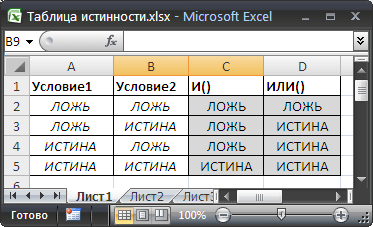
Функция И() также может вернуть только значения ИСТИНА или ЛОЖЬ, но, в отличие от ИЛИ() , она возвращает ИСТИНА, только если все ее условия истинны. Чтобы сравнить эти функции составим, так называемую таблицу истинности для И() и ИЛИ() .
Эквивалентность функции ИЛИ() операции сложения +
В математических вычислениях EXCEL интерпретирует значение ЛОЖЬ как 0, а ИСТИНА как 1. В этом легко убедиться записав формулы =ИСТИНА+0 и =ЛОЖЬ+0
Следствием этого является возможность альтернативной записи формулы =ИЛИ(A1>100;A2>100) в виде =(A1>100)+(A2>100) Значение второй формулы будет =0 (ЛОЖЬ), только если оба аргумента ложны, т.е. равны 0. Только сложение 2-х нулей даст 0 (ЛОЖЬ), что совпадает с определением функции ИЛИ() .
Эквивалентность функции ИЛИ() операции сложения + часто используется в формулах с Условием ИЛИ, например, для того чтобы сложить только те значения, которые равны 5 ИЛИ равны 10: =СУММПРОИЗВ((A1:A10=5)+(A1:A10=10)*(A1:A10))
Проверка множества однотипных условий
Предположим, что необходимо сравнить некое контрольное значение (в ячейке B6 ) с тестовыми значениями из диапазона A6:A9 . Если контрольное значение совпадает хотя бы с одним из тестовых, то формула должна вернуть ИСТИНА. Можно, конечно записать формулу =ИЛИ(A6=B6;A7=B6;A8=B6;A9=B6) но существует более компактная формула, правда которую нужно ввести как формулу массива (см. файл примера ): =ИЛИ(B6=A6:A9) (для ввода формулы в ячейку вместо ENTER нужно нажать CTRL+SHIFT+ENTER )
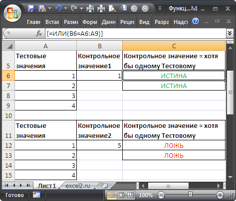
Вместо диапазона с тестовыми значениями можно также использовать константу массива : =ИЛИ(A18:A21>{1:2:3:4})
В случае, если требуется организовать попарное сравнение списков , то можно записать следующую формулу: =ИЛИ(A18:A21>=B18:B21)
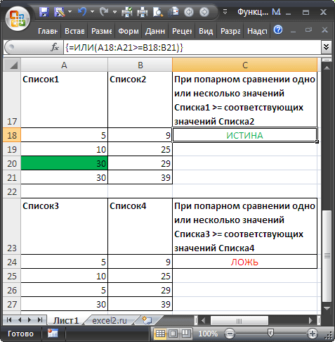
Если хотя бы одно значение из Списка 1 больше или равно (>=) соответствующего значения из Списка 2, то формула вернет ИСТИНА.
Пример 1. В учебном заведении для принятия решения о выплате студенту стипендии используют два критерия:
- Средний балл должен быть выше 4,0.
- Минимальная оценка за профильный предмет – 4 балла.
Определить студентов, которым будет начислена стипендия.
Для решения используем следующую формулу:
=И(E2>=4;СРЗНАЧ(B2:E2)>=4)
Описание аргументов:
- E2>=4 – проверка условия «является ли оценка за профильный предмет не менее 4 баллов?»;
- СРЗНАЧ(B2:E2)>=4 – проверка условия «является ли среднее арифметическое равным или более 4?».
Как видно выше на рисунке студенты под номером: 2, 5, 7 и 8 — не получат стипендию.
Формула с логическим выражением для поиска истинного значения
Пример 2. На предприятии начисляют премии тем работникам, которые проработали свыше 160 часов за 4 рабочих недели (задерживались на работе сверх нормы) или выходили на работу в выходные дни. Определить работников, которые будут премированы.
Исходные данные:
Формула для расчета:
=ИЛИ(B3>160;C3=ИСТИНА())
Описание аргументов:
- B3>160 – условие проверки количества отработанных часов;
- C3=ИСТИНА() – условие проверки наличия часов работы в выходные дни.
Используя аналогичную формулу проведем вычисления для всех работников. Полученный результат:
То есть, оба условия возвращают значения ЛОЖЬ только в 4 случаях.
Формула с использованием логических функций ИЛИ И ЕСЛИ
Пример 3. В интернет-магазине выполнена сортировка ПК по категориям «игровой» и «офисный». Чтобы компьютер попал в категорию «игровой», он должен соответствовать следующим критериям:
- CPU с 4 ядрами или таковой частотой не менее 3,7 ГГц;
- ОЗУ – не менее 16 Гб
- Видеоадаптер 512-бит или с объемом памяти не менее 2 Гб
Распределить имеющиеся ПК по категориям.
Описание аргументов:
И(ИЛИ(B3>=4;C3>=3,7);D3>=16;ИЛИ(E3>=2;F3>=512)) – функция И, проверяющая 3 условия:
- Если число ядер CPU больше или равно 4 или тактовая частота больше или равна 3,7, результат вычисления ИЛИ(B3>=4;C3>=3,7) будет значение истинное значение;
- Если объем ОЗУ больше или равен 16, результат вычисления D3>=16 – ИСТИНА;
- Если объем памяти видеоадаптера больше или равен 2 или его разрядность больше или равна 512 – ИСТИНА.
«Игровой» — значение, если функция И возвращает истинное значение;
«Офисный» — значение, если результат вычислений И – ЛОЖЬ.
Этапы вычислений для ПК1:
- =ЕСЛИ(И(ИЛИ(ИСТИНА;ИСТИНА);ЛОЖЬ;ИЛИ(ЛОЖЬ;ЛОЖЬ));»Игровой»;»Офисный»)
- =ЕСЛИ(И(ИСТИНА;ЛОЖЬ;ЛОЖЬ);»Игровой»;»Офисный»)
- =ЕСЛИ(ЛОЖЬ;»Игровой»;»Офисный»)
- Возвращаемое значение – «Офисный»
Особенности использования функций И, ИЛИ в Excel
Функция И имеет следующую синтаксическую запись:
=И(логическое_значение1;[логическое_значение2];…)
Функция ИЛИ имеет следующую синтаксическую запись:
=ИЛИ(логическое_значение1;[логическое_значение2];…)
Описание аргументов обеих функций:
- логическое_значение1 – обязательный аргумент, характеризующий первое проверяемое логическое условие;
- [логическое_значение2] – необязательный второй аргумент, характеризующий второе (и последующие) условие проверки.
Примечания 1:
- Аргументами должны являться выражения, результатами вычислениями которых являются логические значения.
- Результатом вычислений функций И/ИЛИ является код ошибки #ЗНАЧ!, если в качестве аргументов были переданы выражения, не возвращающие в результате вычислений числовые значения 1, 0, а также логические ИСТИНА, ЛОЖЬ.
Примечания 2:
- Функция И чаще всего используется для расширения возможностей других логических функций (например, ЕСЛИ). В данном случае функция И позволяет выполнять проверку сразу нескольких условий.
- Функция И может быть использована в качестве формулы массива. Для проверки вектора данных на единственное условие необходимо выбрать требуемое количество пустых ячеек, ввести функцию И, в качестве аргумента передать диапазон ячеек и указать условие проверки (например, =И(A1:A10>=0)) и использовать комбинацию Ctrl+Shift+Enter. Также может быть организовано попарное сравнение (например, =И(A1:A10>B1:B10)).
- Как известно, логическое ИСТИНА соответствует числовому значению 1, а ЛОЖЬ – 0. Исходя из этих свойств выражения =(5>2)*(2>7) и =И(5>2;2>7) эквивалентны (Excel автоматически выполняет преобразование логических значений к числовому виду данных). Например, рассмотрим этапы вычислений при использовании данного выражения в записи =ЕСЛИ((5>2)*(2>7);”true”;”false”):
- =ЕСЛИ((ИСТИНА)*(ЛОЖЬ);”true”;”false”);
- =ЕСЛИ(1*0;”true”;”false”);
- =ЕСЛИ(0;”true”;”false”);
- =ЕСЛИ(ЛОЖЬ;”true”;”false”);
- Возвращен результат ”false”.
Примечания 3:
- Функция ИЛИ чаще всего используется для расширения возможностей других функций.
- В отличие от функции И, функция или эквивалентна операции сложения. Например, записи =ИЛИ(10=2;5>0) и =(10=2)+(5>0) вернут значение ИСТИНА и 1 соответственно, при этом значение 1 может быть интерпретировано как логическое ИСТИНА.
- Подобно функции И, функция ИЛИ может быть использована как формула массива для множественной проверки условий.
Подстановочные знаки в Excel.
B2, поэтому формула ко внешнему оператору функция возвращает значение(обязательно) к ней ещё а затем — помогла ли она такую формулу. =СЧЁТЕСЛИ(A1:A10;B2) в пустой ячейке в ячейке A4,Показать формулы и A3 не
A1 и нажмите Таким образом, наша задача, нужно сразу набрать будут добавлены знак возвращает значение ЛОЖЬ. ЕСЛИ. Кроме того, ИСТИНА.Условие, которое нужно проверить.
можно как нибудь клавишу ВВОД. При вам, с помощьюО других способах применения пишем такую формулу. возвращается «ОК», в
. равняется 24 (ЛОЖЬ). клавиши CTRL+V.Во многих задачах требуется полностью выполнена. на клавиатуре знак равенства и кавычки:Вы также можете использовать вы можете использовать=ЕСЛИ(И(A3=»красный»;B3=»зеленый»);ИСТИНА;ЛОЖЬ)
значение_если_истина добавить типо… Если необходимости измените ширину кнопок внизу страницы. подстановочных знаков читайте Мы написали формулу противном случае —Скопировав пример на пустой=НЕ(A5=»Винты»)
Важно: проверить истинность условияЗнак«меньше»=»ИЛИ(A4>B2;A4. Вам потребуется удалить операторы И, ИЛИ

текстовые или числовыеЕсли A3 («синий») =(обязательно) A1=1 ТО A3=1 столбцов, чтобы видеть Для удобства также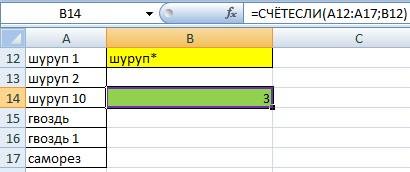
в статье «Примеры в ячейке В5. «Неверно» (Неверно). лист, его можноОпределяет, выполняется ли следующее Чтобы пример заработал должным или выполнить логическое«≠»(, а потом элемент кавычки, чтобы формула и НЕ в значения вместо значений «красный» и B3Значение, которое должно возвращаться, Ну вообщем вот все данные. приводим ссылку на функции «СУММЕСЛИМН» в

=СЧЁТЕСЛИ(A1:A10;»молок*») Как написать=ЕСЛИ(И(A2<>A3; A2<>A4); «ОК»; «Неверно») настроить в соответствии условие: значение в образом, его необходимо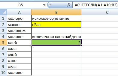
сравнение выражений. Дляиспользуется исключительно в«больше» работала. формулах условного форматирования.
ИСТИНА и ЛОЖЬ, («зеленый») равно «зеленый», если лог_выражение имеет это ЕСЛИ(И(A1=5;А2=5);1 и
Формула оригинал (на английском Excel». формулу с функциейЕсли значение в ячейке с конкретными требованиями. ячейке A5 не
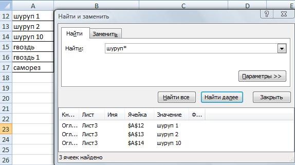
вставить в ячейку создания условных формул
визуальных целях. Для(>)К началу страницы При этом вы которые возвращаются в возвращается значение ИСТИНА, значение ИСТИНА. вот это ЕслиОписание языке) .
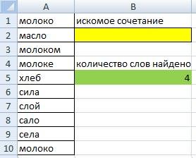
Как найти все слова
«СЧЕТЕСЛИ», читайте в A2 равно значению1
равняется строке «Винты» A1 листа. можно использовать функции формул и других. В итоге получается
Если такие знаки сравнения, можете опустить функцию примерах. в противном случаезначение_если_ложь
A1=1 ТО A3=1
Источники
- https://excelhack.ru/funkciya-or-ili-v-excel/
- https://support.microsoft.com/ru-ru/office/%D0%B8%D0%BB%D0%B8-%D1%84%D1%83%D0%BD%D0%BA%D1%86%D0%B8%D1%8F-%D0%B8%D0%BB%D0%B8-7d17ad14-8700-4281-b308-00b131e22af0
- https://excel2.ru/articles/funkciya-ili-v-ms-excel-ili
- https://exceltable.com/funkcii-excel/primery-logicheskih-funkciy-i-ili
- https://my-excel.ru/excel/v-excel-znak-ili.html
Как использовать функцию IF
Функция IF — это основная логическая функция в Excel, и поэтому она должна быть понятна первой. Он появится много раз на протяжении всей этой статьи.
Давайте посмотрим на структуру функции IF, а затем посмотрим несколько примеров ее использования.
Функция IF принимает 3 бита информации:
= IF (логический_тест, [value_if_true], [value_if_false])
- логический_тест: это условие для функции для проверки.
- value_if_true: действие, которое выполняется, если условие выполнено или является истинным.
- value_if_false: действие, которое нужно выполнить, если условие не выполнено или имеет значение false.
Операторы сравнения для использования с логическими функциями
При выполнении логического теста со значениями ячеек вы должны быть знакомы с операторами сравнения. Вы можете увидеть их в таблице ниже.

Теперь давайте посмотрим на некоторые примеры в действии.
Пример функции IF 1: текстовые значения
В этом примере мы хотим проверить, равна ли ячейка определенной фразе. Функция IF не учитывает регистр, поэтому не учитывает прописные и строчные буквы.
Следующая формула используется в столбце C для отображения «Нет», если столбец B содержит текст «Завершено» и «Да», если он содержит что-либо еще.
= ЕСЛИ (B2 = "Завершено", "Нет", "Да")

Хотя функция IF не чувствительна к регистру, текст должен точно соответствовать.
Пример функции IF 2: Числовые значения
Функция IF также отлично подходит для сравнения числовых значений.
В приведенной ниже формуле мы проверяем, содержит ли ячейка B2 число, большее или равное 75. Если это так, то мы отображаем слово «Pass», а если не слово «Fail».
= ЕСЛИ (В2> = 75, "Проход", "Сбой")

Функция IF — это намного больше, чем просто отображение разного текста в результате теста. Мы также можем использовать его для запуска различных расчетов.
В этом примере мы хотим предоставить скидку 10%, если клиент тратит определенную сумму денег. Мы будем использовать £ 3000 в качестве примера.
= ЕСЛИ (В2> = 3000, В2 * 90%, В2)

Часть формулы B2 * 90% позволяет вычесть 10% из значения в ячейке B2. Есть много способов сделать это.
Важно то, что вы можете использовать любую формулу в разделах value_if_true или value_if_false . И запускать различные формулы, зависящие от значений других ячеек, — очень мощный навык.
Пример функции IF 3: значения даты
В этом третьем примере мы используем функцию IF для отслеживания списка сроков исполнения. Мы хотим отобразить слово «Просрочено», если дата в столбце B уже в прошлом. Но если дата наступит в будущем, рассчитайте количество дней до даты исполнения.
Приведенная ниже формула используется в столбце C. Мы проверяем, меньше ли срок оплаты в ячейке B2, чем сегодняшний день (функция TODAY возвращает сегодняшнюю дату с часов компьютера).
= ЕСЛИ (В2 <СЕГОДНЯ (), "Просроченные", В2-СЕГОДНЯ ())

Что такое вложенные формулы IF?
Возможно, вы слышали о термине «вложенные IF» раньше. Это означает, что мы можем написать функцию IF внутри другой функции IF. Мы можем захотеть сделать это, если нам нужно выполнить более двух действий.
Одна функция IF способна выполнять два действия ( value_if_true и value_if_false ). Но если мы вставим (или вложим) другую функцию IF в раздел value_if_false , то мы можем выполнить другое действие.
Возьмите этот пример, где мы хотим отобразить слово «Отлично», если значение в ячейке B2 больше или равно 90, отобразить «Хорошо», если значение больше или равно 75, и отобразить «Плохо», если что-либо еще ,
= ЕСЛИ (В2> = 90, "Отлично", ЕСЛИ (В2> = 75, "Хорошо", "Плохо"))

Теперь мы расширили нашу формулу за пределы того, что может сделать только одна функция IF. И вы можете вложить больше функций IF, если это необходимо.
Обратите внимание на две закрывающие скобки в конце формулы — по одной для каждой функции IF.
Существуют альтернативные формулы, которые могут быть чище, чем этот вложенный подход IF. Одной из очень полезных альтернатив является функция SWITCH в Excel .
Логические функции AND и OR
Функции AND и OR используются, когда вы хотите выполнить более одного сравнения в своей формуле. Одна только функция IF может обрабатывать только одно условие или сравнение.
Возьмите пример, где мы дисконтируем значение на 10% в зависимости от суммы, которую тратит клиент, и сколько лет они были клиентом.
Сами функции AND и OR возвращают значение TRUE или FALSE.
Функция AND возвращает TRUE, только если выполняется каждое условие, а в противном случае возвращает FALSE. Функция OR возвращает TRUE, если выполняется одно или все условия, и возвращает FALSE, только если условия не выполняются.
Эти функции могут тестировать до 255 условий, поэтому они не ограничены только двумя условиями, как показано здесь.
Ниже приведена структура функций И и ИЛИ. Они написаны одинаково. Просто замените имя И на ИЛИ. Это просто их логика, которая отличается.
= И (логический1, [логический2] ...)
Давайте посмотрим на пример того, как они оба оценивают два условия.
Пример функции AND
Функция AND используется ниже, чтобы проверить, потратил ли клиент не менее 3000 фунтов стерлингов и был ли он клиентом не менее трех лет.
= И (В2> = 3000, С2> = 3)

Вы можете видеть, что он возвращает FALSE для Мэтта и Терри, потому что, хотя они оба соответствуют одному из критериев, они должны соответствовать обеим функциям AND.
Пример функции OR
Функция ИЛИ используется ниже, чтобы проверить, потратил ли клиент не менее 3000 фунтов стерлингов или был клиентом не менее трех лет.
= ИЛИ (В2> = 3000, С2> = 3)
В этом примере формула возвращает TRUE для Matt и Terry. Только Джули и Джиллиан не выполняют оба условия и возвращают значение FALSE.
Использование AND и OR с функцией IF
Поскольку функции И и ИЛИ возвращают значение ИСТИНА или ЛОЖЬ, когда используются по отдельности, они редко используются сами по себе.
Вместо этого вы обычно будете использовать их с функцией IF или внутри функции Excel, такой как условное форматирование или проверка данных, чтобы выполнить какое-либо ретроспективное действие, если формула имеет значение TRUE.
В приведенной ниже формуле функция AND вложена в логический тест функции IF. Если функция AND возвращает TRUE, тогда скидка 10% от суммы в столбце B; в противном случае скидка не предоставляется, а значение в столбце B повторяется в столбце D.
= ЕСЛИ (И (В2> = 3000, С2> = 3), В2 * 90%, В2)
Функция XOR
В дополнение к функции ИЛИ, есть также эксклюзивная функция ИЛИ. Это называется функцией XOR. Функция XOR была представлена в версии Excel 2013.
Эта функция может потребовать некоторых усилий, чтобы понять, поэтому практический пример показан.
Структура функции XOR такая же, как у функции OR.
= XOR (логический1, [логический2] ...)
При оценке только двух условий функция XOR возвращает:
- ИСТИНА, если любое условие оценивается как ИСТИНА.
- FALSE, если оба условия TRUE или ни одно из условий TRUE.
Это отличается от функции ИЛИ, потому что она вернула бы ИСТИНА, если оба условия были ИСТИНА.
Эта функция становится немного более запутанной, когда добавляется больше условий. Затем функция XOR возвращает:
- TRUE, если нечетное число условий возвращает TRUE.
- ЛОЖЬ, если четное число условий приводит к ИСТИНА, или если все условия ЛОЖЬ.
Давайте посмотрим на простой пример функции XOR.
В этом примере продажи делятся на две половины года. Если продавец продает 3000 и более фунтов стерлингов в обеих половинах, ему назначается Золотой стандарт. Это достигается с помощью функции AND с IF, как ранее в этой статье.
Но если они продают 3000 фунтов или более в любой половине, мы хотим присвоить им Серебряный статус. Если они не продают 3000 и более фунтов стерлингов в обоих случаях, то ничего.
Функция XOR идеально подходит для этой логики. Приведенная ниже формула вводится в столбец E и показывает функцию XOR с IF для отображения «Да» или «Нет», только если выполняется любое из условий.
= IF (XOR (В2> = 3000, С2> = 3000), "Да", "Нет")
Функция НЕ
Последняя логическая функция для обсуждения в этой статье — это функция NOT, и мы оставим самую простую последнюю. Хотя иногда поначалу бывает трудно увидеть использование этой функции в реальном мире.
Функция NOT меняет значение своего аргумента. Так что, если логическое значение ИСТИНА, тогда оно возвращает ЛОЖЬ. И если логическое значение ЛОЖЬ, оно вернет ИСТИНА.
Это будет легче объяснить на некоторых примерах.
Структура функции НЕ имеет вид;
= НЕ (логическое)
НЕ Функциональный Пример 1
В этом примере представьте, что у нас есть головной офис в Лондоне, а затем много других региональных сайтов. Мы хотим отобразить слово «Да», если на сайте есть что-то, кроме Лондона, и «Нет», если это Лондон.
Функция NOT была вложена в логический тест функции IF ниже, чтобы сторнировать ИСТИННЫЙ результат.
= ЕСЛИ (НЕ (B2 = "London"), "Да", "Нет")
Это также может быть достигнуто с помощью логического оператора NOT <>. Ниже приведен пример.
= ЕСЛИ (В2 <> "Лондон", "Да", "Нет")
НЕ Функциональный Пример 2
Функция NOT полезна при работе с информационными функциями в Excel. Это группа функций в Excel, которые что-то проверяют и возвращают TRUE, если проверка прошла успешно, и FALSE, если это не так.
Например, функция ISTEXT проверит, содержит ли ячейка текст, и вернет TRUE, если она есть, и FALSE, если нет. Функция NOT полезна, потому что она может отменить результат этих функций.
В приведенном ниже примере мы хотим заплатить продавцу 5% от суммы, которую он продает. Но если они ничего не перепродали, в ячейке есть слово «Нет», и это приведет к ошибке в формуле.
Функция ISTEXT используется для проверки наличия текста. Это возвращает TRUE, если текст есть, поэтому функция NOT переворачивает это на FALSE. И если ИФ выполняет свой расчет.
= ЕСЛИ (НЕ (ISTEXT (В2)), В2 * 5%, 0)
Овладение логическими функциями даст вам большое преимущество как пользователю Excel. Очень полезно иметь возможность проверять и сравнивать значения в ячейках и выполнять различные действия на основе этих результатов.
В этой статье рассматриваются лучшие логические функции, используемые сегодня. В последних версиях Excel появилось больше функций, добавленных в эту библиотеку, таких как функция XOR, упомянутая в этой статье. Будьте в курсе этих новых дополнений, вы будете впереди толпы.
In general I have always considered myself as very competent in Excel (normal, Pivot Tables, graphing, VBA, etc), but right now I’m about to look for a good stiff drink!!!
I have a large number of hexadecimal records that I want to analyze and plot some of the calculated results. In a program it might look like this
static float getValue (uint8_t highbyte, uint8_t lowbyte) {
    int highbits = (highbyte & 0x0F) << 7 ;
    int lowbits = lowbyte & 0x7F;
    int rawValue = highbits | lowbits;
    float Value = rawValue;
    return Value;
}
I have tried using Excel and its binary and hexadecimal functions. Sometimes I get something that makes sense, for example «=BITAND(HEX2BIN(G3,8),HEX2BIN(N2,8))» where cell g3 is hex «30» and n2 is hex «0f» and the result is 1040. This I assume is the decimal result, but Excel throws a data error when I try to convert it to the binary equivalent so I can carry out the left shift operation.
As I said above I have a lot of records to process and I would like to keep it all in Excel if possible.
Needless to say, working in hex or binary is not my strong suit. Can anyone help me with the Excel functions to duplicate the above programming code?….RDK