
Much of the data that you use Excel to analyze comes in a list form. You might need to sort the data, filter it, sum it, and perhaps even chart it. Excel tables provide superior tools for working with data in list form.
If you want to sum columns of data automatically so that the totals show only the sum of visible cells (for example), Excel’s Tables features can do it. And if you want to format any Excel data in just a couple of quick steps, Excel’s Tables features can handle that task, too. And as for using a form instead of punching numbers into ordinary spreadsheet cells, Tables once again can do the job.
Here are my top 10 secrets for managing lists of data using Excel Tables.
1. Create a Table in Any of Several Ways
The first step in learning how to work with Excel’s Tables features is to use the program to create a table. You’ll need a list with column headings and (if you wish) row headings. Select the data, including the heading rows and columns, and click Insert > Table. Visually confirm that the range you’ve selected is correct, click the My table has headers checkbox, and click OK. Excel will then create a formatted table for you. If you would prefer to choose a particular table format, select the same data area and click Home (instead of Insert); then choose a table style from the Table Styles gallery.
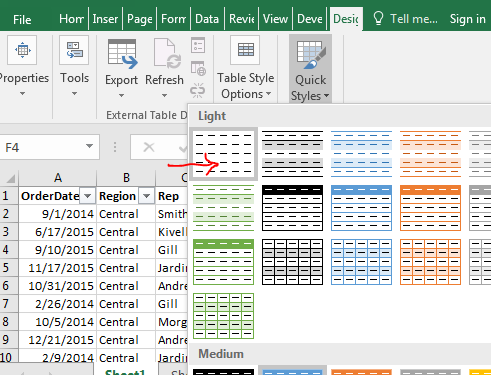
2. Remove the Filter Arrows
Click the Filter option to toggle the display of the filter arrows on or off. Microsoft
When you want to use some features of an Excel table, but you don’t plan to filter or sort your data, you can hide the filter arrows. To do this, click somewhere inside the table and then click Data > Sort & Filter > Filter. Now you can toggle between hiding the arrows with one click and revealing them with the next. The shortcut keystroke combination Shift-Ctrl-L accomplishes the same thing.
3. Take the Format but Ditch the Table
Formatting data as an Excel table is the quickest way to achieve a neatly formatted range of cells in Excel. The only potential problem is that it may seem that you can’t get the formatting without getting all the unwanted table features as well. But while this limitation is technically true, you don’t have to keep the table features if you don’t want them. To borrow a table style for any worksheet, first create the data as a table, making sure to choose your preferred table style for formatting it.
Next, click inside the table and then click Table Tools > Design > Convert to Range. Click Yes when Excel prompts you with ‘Do you want to convert the table to a normal range?’ and the table will revert to being a regular range—but with its attractive formatting intact.
4. Fix Ugly Column Headings
The filter arrows in an Excel table’s column headings look downright ugly when those headings are right-justified. The arrows cover the rightmost characters in the headings, and there is no obvious way to fix the problem. The workaround is to indent the content from the right side of the cell. To do this, select the cells containing the headings that are partly hidden and click Home > Increase Indent. If the cell contents respond by jumping to the left edge of the cell, click Home > Align Right to return them to right justification. Click Increase Indent more than once as necessary to position the heading text well clear of the filter arrows.
5. Add New Rows to a Table
Rows in a table behave a little differently from rows in a regular worksheet. If you need to add a new row to a table, and if the Totals row is not visible, click in the bottom right cell in the table and press the Tab key. This simple procedure adds a new row to the table, just as it would if you were working with a Word table.
To add rows to the end of a table, drag the small indicator in the bottom right corner of the table to add more rows and more adjacent columns, if desired. To add a row inside a table, click in a cell either above or below where the row should be inserted and click either Home > Insert > Insert Table Row Above or Home > Insert > Insert Table Row Below, depending on where you want the new row to appear. The table’s formatting will automatically adjust so that the new row is correctly formatted.
Next page: How to calculate accurate column totals.
6. Calculate Accurate Totals
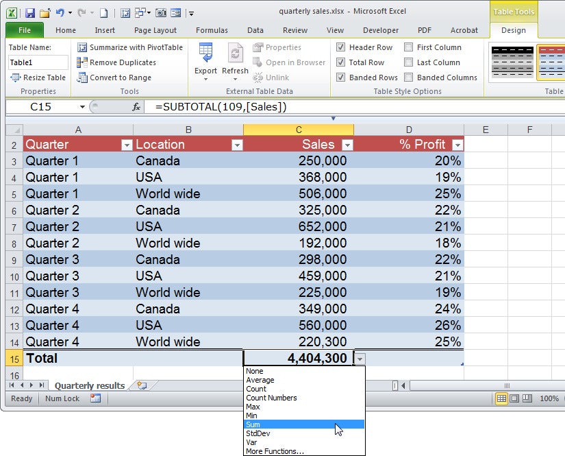
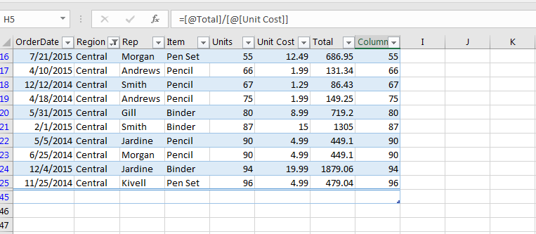
Anyone who has ever tried to use the SUM function to total a column of data in which some of the rows are hidden has received a nasty surprise: The SUM function calculates the total of all of the cells in a range, whether they’re visible or not. This characteristic of the function means that the result won’t be the total of the numbers in the visible rows—and that discrepancy can be a huge problem. The way tyo avoid this difficulty is to use the SUBTOTAL function instead. Excel will do this automatically when you use its Total row feature for your table.
When you want to add a total row to the table, click inside the table, right-click, and choose Table > Totals Row; or click inside the table and click Table Tools > Design > Total Row. In either case, a total row will appear at the foot of the table. If the last column contains numerical values, Excel will automatically use a SUBTOTAL function to sum them.
To add a total to any other column, click in the appropriate cell in the Total row, and in the drop-down menu click SUM. This operation will add a SUBTOTAL formula to the cell that will total only visible values when the table is filtered. You may choose other calculation options from this drop-down list, including Min, Max, Count, and Average.
7. Create a Chart From Table Data
One significant benefit of formatting a list as a table is that charts created from table data change dynamically when you add data to or remove data from the table. So a column chart that charts the values in a range will expand to incorporate new values when you add them to the table. This is the case whether you add data to the bottom of the table or introduce a new column to the right of it. Creating a chart based on the table is the same as creating any chart in Excel—only the behavior of the chart is different. Tables of this type are extremely useful when you work with data that expands or contracts over time.
8. Enter Data Using a Simple Form
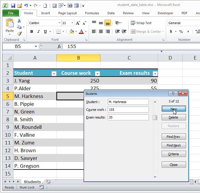
Typing lots of data across a wide table can be quite cumbersome; often, entering data into a form is easier. Earlier versions of Excel included a handy Form tool; that tool is still available, but you won’t find it on the Ribbon. To make it easier to find, you can add it to Excel’s Quick Access Toolbar: Click File > Options > Quick Access Toolbar. In the Choose Commands From list, click All Commands and then scroll down and click Form…. Click Add to add the tool to the Quick Access Toolbar, and then click OK.
To use the form, click somewhere inside your table and then click the Form button to display a form dialog area. The form heading is the sheet name, and the form contains boxes where you can preview the current form data and add new data. To add new data, click New and type the data into the relevant text boxes. To view the form data, click Find Prev or Find Next to move through the data one row (record) at a time. To exit the form, click Close.
9. Sort and Filter Table Data
One key feature of Excel’s tables is their ability to sort and filter the data in the table. To perform either of these actions, click the down arrow to the right of any table column and then choose a Sort or Filter option. The two Sort options available are ‘ascending’ and ‘descending’. The Filter options vary depending on whether you’re working with a column of numbers, text, or dates.
You can then select from among a number of predefined options, or click Custom Filter and build your own. Alternatively you can create complex filters such as AND and OR filters. For example, locating values in a column that are less than $200,000 or more than $400,000 involves using an OR filter. To create it, click Custom Filter and then build both parts of the search in the dialog area, making sure to click the OR option. Similarly you can create AND filters that work across two columns, thereby enabling you to display information such as “All entries for Canada, where sales are greater than $300,000.” In this case you would select to view only ‘Canada’ in the Location column. In the Sales column, click Numbers Filters > Custom Filter > is greater than, type 300000 and click OK.
Any column that has a filter in place will show a filter icon instead of the downward-pointing triangle, so you can see at a glance where the filters are. To clear a filter, click the Filter icon and click Clear filter from; or click Home > Sort & Filter > Clear to clear all filters from all columns in the table.
10. Create Complex OR Searches Across Multiple Columns
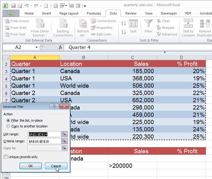
One type of search that you can’t build using the menu options is an OR search of the type “All entries for Canada or where sales are greater than $200,000.” Consequently you must write a search instruction of this type in a different way. To do so, first copy the table heading row and paste it a few rows immediately below your table. Beneath these headings, in the Location column, type =”=Canada” and in the second row, in the Sales column, type >200000. Click inside the table, click Data > Advanced > Filter the list, in-place. Confirm that the List range is the table range, and set the Criteria Range to an area covering the second set of headings and the two data rows below it. Then click OK to filter the list.
If you’ve enjoyed this article, check out these related stories:
• “How to Create Advanced Microsoft Excel Spreadsheets”
• “Work Faster in Microsoft Excel: 10 Secret Tricks”
• “Make Data Entry Easier in Microsoft Excel: 10 Tricks”
When was the last time you used excel tables? Do you know how powerful excel tables are?
If you have never or not recently used excel tables, it could be because you have not realized how powerful they are in data analysis.
By reading below 7 excel table’s secrets, your answer to above question will always be recent.
-
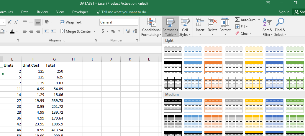
Simple to create —Ctrl + T
There are 2 ways of creating an excel table: Select any cell on your data, Go to HOME tab, under styles, click format as table and then select table format. Finally, click OK on the “FormatAsTable” Dialogue box that appears. This is the most common method used but it is too long.
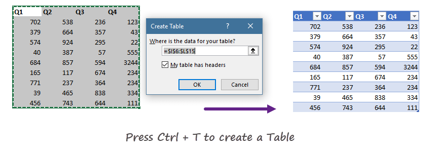
The simplest way to create an excel table is by use of a shortcut “Ctrl +T”. Select anywhere in your data then Ctrl +T and then click OK on Create Table Dialogue.

-
The best data source for Pivot tables
One of the biggest mistakes excel users make when using pivot tables is the failure to include in the pivot table analysis extra rows or columns added to their data source. This can be easily sorted by use of Excel tables.
Excel tables automatically expand to include the new rows and columns in the table saving time to check if you have included all data. All that is required is to hit refresh in and your pivot table is fully updated.
Furthermore, you can easily convert a table to a pivot table with just one click. Under Table tools in Design tab, Click Summarize with PivotTable. That’s All!

-
Use of Slicers to Filter table
Slicers are excellent tools for data visualization, especially creating dashboards. These work best when data is formatted as an excel table.
To easily filter table data using slicers, select the table, Under Design tab, Select insert Slicer

Select the column you want to create slicers for and then OK.
 az
az
Excel creates a Slicer as shown in the image below which is an excellent way to filter tables:

-
Easily create Summaries
You can easily create a one-line summary on the table without writing any formula.
To do this, Under Design Tab, tick Total Row.

Click the total figure and you will find a drop down that has more summary types you can apply by just clicking on any of them.

-
Create Dynamically expanding Charts
Manually updating chart data range is hectic and prone to errors. With Excel table, your chart data range is automatically expanded.
To do this, Select Columns in the table to create a chart, then Insert the chart. As Excel tables automatically expand to include the new rows and columns in the table, so will the chart labels and values be expanded.
This is far much easier than using the indirect and offset functions to create a dynamic chart.
-
The quickest way to insert Running Totals
Running totals are important in data analysis as they show the overall progress. Excel tables structure enables a quick insert of calculated fields which is the best fit for running totals.
For example to add a running totals column in below sales data, just type below simple sum formula on a column adjacent to the last column in the table. When you hit the enter button, excel table instantly applies the formula to all other cells in that table creating a column that contains running totals.
This is possible because of the structured reference format of the formula, a feature unique in excel tables.

With just that one formula, you get below accurate running totals

-
Excel table’s awesome data referencing
Most Excel users are used to cell referencing which is mostly hard to understand.
Excel tables introduced structured references which are easily explainable especially in a formula created outside the excel table.
Structured reference syntax = Table name [Column name]
For example, in below formula, you can tell the count range is data contained in products column which is in a table called sales.
=COUNTIF(Sales[Product],"Paper")

In case you need to drag your formula across, the easiest way to create a Column Absolute reference is to create a duplicate column name separated by a full colon.
=COUNTIF(Sales[[Product]:[Product]],G1)

Conclusion:
As you can see from above discussion, the whole aim of excel tables is to make a data analyst life simple.
So, does your life seem complicated?
Check out if you are using Excel tables and include them in your daily excel work.
For further reading check out this article: https://support.office.com/en-us/article/Using-structured-references-with-Excel-tables-f5ed2452-2337-4f71-bed3-c8ae6d2b276e
Interesting Links
4 WAYS TO SUM DATA BY WEEK NUMBER
Nothing beats the time-saving awesomeness of the perfect Excel template.
Whether you’re managing a team of employees or a busy household, being able to simply plug in your data and go means your work gets done faster, your projects run smoother, and you’re the most organized person in the room.
But finding the right template can be time-consuming on its own.
Luckily, you can get started ASAP because we’ve compiled a list of 52 free Excel templates to help make your life easier today.
Level up your Excel skills
Become a certified Excel ninja with GoSkills bite-sized courses
Start free trial
Our list has you covered with template picks spanning 7 categories:
- Project management
- Money management
- Planning ahead
- Buying a house
- Personal weight loss
- Business management
- Business planning
Skip ahead to the sections you’re interested in or check each one out to see what you’re missing.
Looking for more templates? Check out these free downloadable Word resume templates and PowerPoint templates.
To kick things off, let’s start with 7 project management templates your team can’t afford to go without.
Project management
1. Timeline template
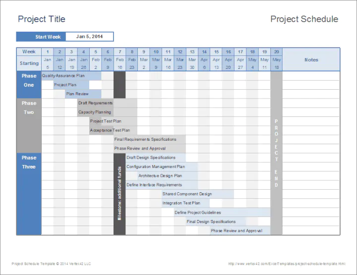 Most of us are used to seeing timelines in history class, but they also work well for project management. Timelines give you a general overview of important milestones and key events that everyone on the team should be aware of.
This helps your team stay on the same page throughout the course of your project. If you don’t have time to create your own project timeline, don’t sweat it. Use this template to create one quickly.
2. Gantt Chart template
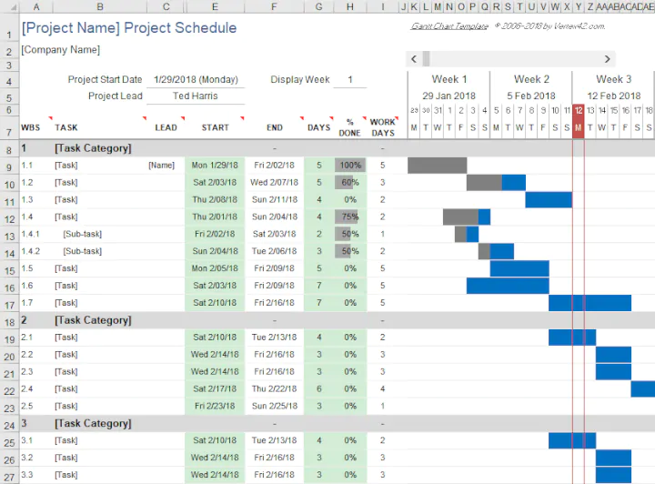 Take your project timeline a step further by using this Gantt Chart free Excel template. This gives you a timeline with a bit more detail. You can mark and see at a glance the start and end times of your project, plus all those important milestones to reach until it’s complete.
Each milestone also has a summary of what needs to be done so there’s no question as to what everyone on your team should be working on and when those deliverables are due.
For the best results, create a general timeline to look at for quick answers, such as when something is due, and your Gantt Chart to see the details of the deliverables before they’re due.
3. To-do list template
Hold your team accountable. Once you have your general timeline created and your Gantt Chart laid out, you’ll need a way to keep your team in the loop with the status of certain deliverables. This to-do list template will help you do just that.
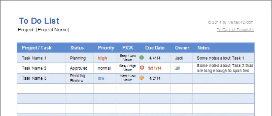
With this template, you can add the project tasks, a status update, the priority level, a due date, who’s in charge, and any relevant notes to ensure that everyone on the team knows what’s going on.
And if any issues come up, you can use this next template.
4. Issue tracking template
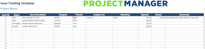 Unfortunately, all projects have their share of issues. It’s important to document these both for learning purposes in the future and figuring out how to solve the issue in the here and now.
This issue tracking template helps you keep a log of what went wrong, when it occurred, who handled the problem, and any relevant notes that may be helpful.
Remember, it’s better to identify the issues and document them now than it is to keep repeating the same mistakes over and over again because you failed to identify a common thread.
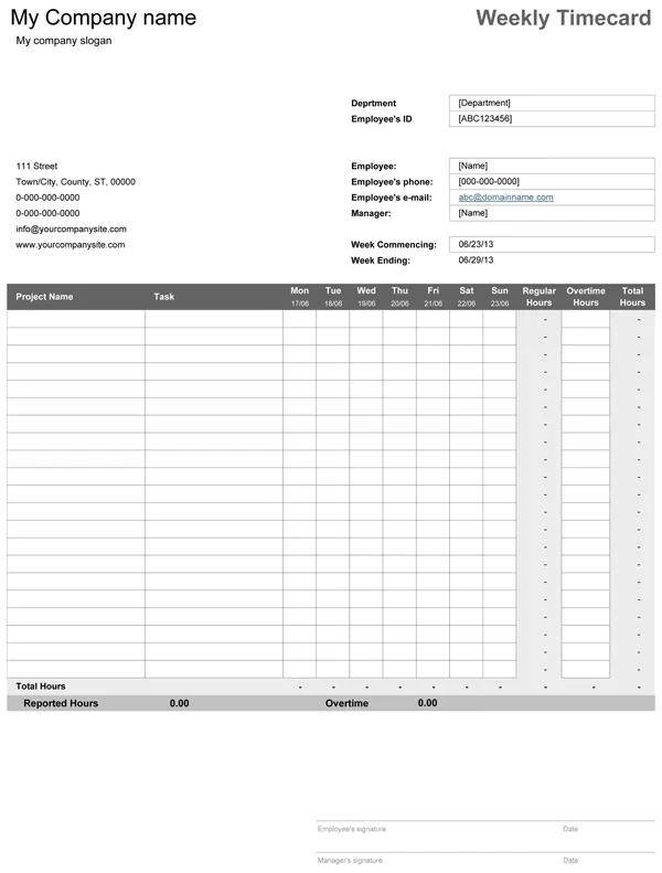
5. Weekly timecard template
 On top of tracking issues, it’s a good idea to also record how long each step in a project is taking your team so you can price your services accordingly. This weekly timecard for projects will give you a better idea of that.
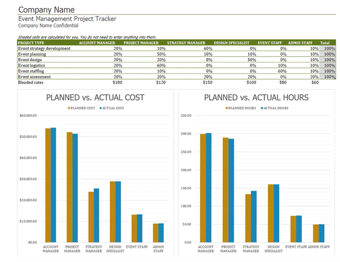
6. Project tracking template
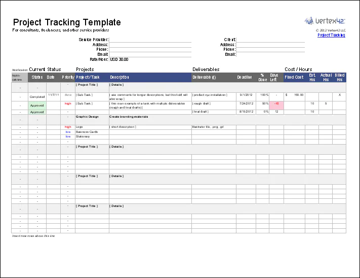 You can also use this project tracking template to gauge if your projects are running on time and within budget.
7. KPI tracking template
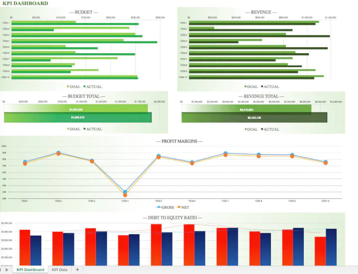 This project KPI tracking template will also help you measure the performance of your projects to ensure you’re hitting the mark every time. After all, you don’t want to learn that you missed your target at the end of a project when it’s too late to do anything about it.
In this next section, I’ll show you the best templates to help you manage your money.
Want to learn more?
Take your Excel skills to the next level with our comprehensive (and free) ebook!
Money management
8. Money management template
 Manage all your finances at a glance. This money management template keeps your finances organized by breaking down your spending into categories such as household, savings, and charitable donations.
9. Personal budget template
 Create a personal budget. On top of managing your spending, you should also track your spending in relation to your budget to see where you can cut down. This personal budget template will make that a breeze.
10. Income and expense template
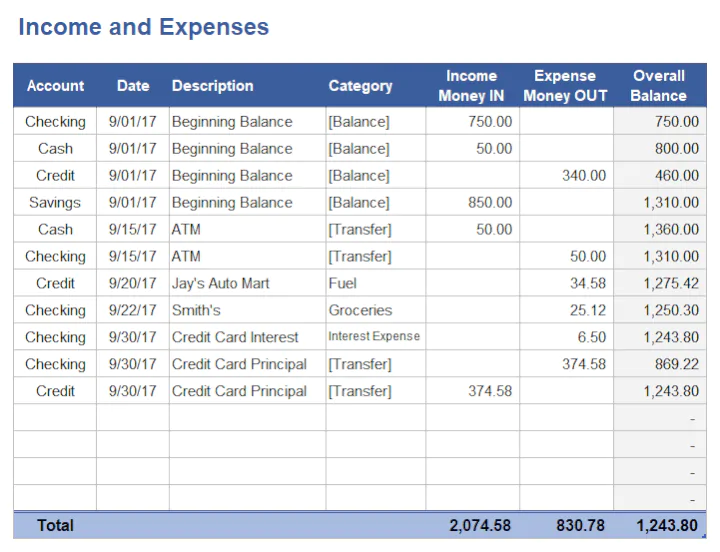 Use this template when you want to compare your income to your expenses. This helps you see if you’re living within your means or not. And if it turns out you aren’t, consider using the personal budget template to fix things.
11. Family budget planner template
 What if you’re managing more than just your own finances? For those in charge of a household, a family budget planner template can help you see an overall view of what your family spends money on throughout the year.
12. Household budget template
 Once you have an idea of where your money goes as a family, you can then start using a household budget template to keep things in control and under budget.
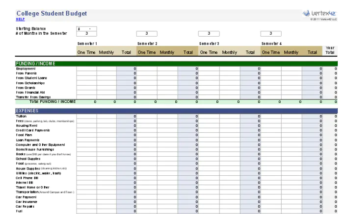
13. College budget template
For students, there’s also this helpful college budget template that tracks where most of your funds are going. Then you’ll know what to expect and how to plan ahead each semester (for the most part).
14. Holiday spending budget template
 The holidays can be a hard hit financially if you’re not careful. With lengthy wish-lists, it’s important to balance what everyone wants with what you can actually afford. This holiday spending budget helps you do that the easy way.
15. Travel budget template
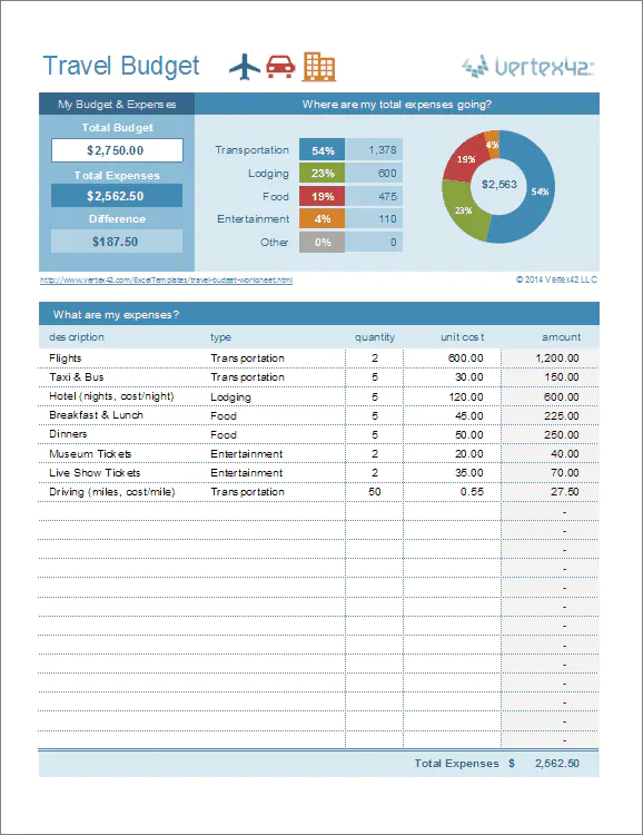 Dream of traveling to a remote beach far away? Use this travel budget template and you’ll be well on your way to making that dream a reality.
16. Kids money management template
 You can also teach your children how to track their allowance, savings, and spending with this helpful money management template for kids.
17. Savings goal template
 If your kids (or you) have a savings goal in mind, use this free Excel template. By tracking exactly how much you save each month, you’ll have a better chance of making progress towards your goal.
18. Wedding budget template
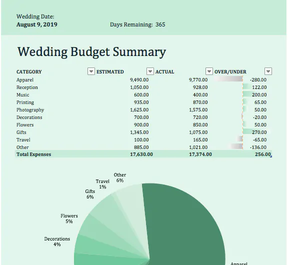 Weddings can also be a costly adventure for many. To ensure you don’t go over budget, check out this free wedding budget template.
19. Get out of debt template
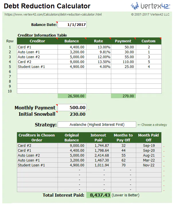 And if wedding bells are not in your immediate plans and getting out from under a mound of debt is, this template has your name on it.
Want to learn more?
Take your Excel skills to the next level with our comprehensive (and free) ebook!
20. Portfolio management template
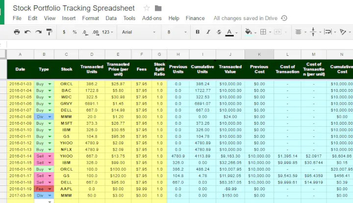 You can also use this portfolio management template to track and maximize how much you earn from your investments.
Up next, I’ll show you how a little planning ahead will make your life smooth sailing down the road.
Planning ahead
21. Meal plan template
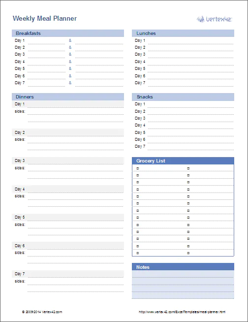 Deciding what to eat after a long day at work is never an easy task. To avoid this headache, meal plan ahead of time using this template, which helps you plan your breakfasts, lunches, and dinners before you even start your work week. It even has a convenient place for you to write down your grocery list.
22. Home remodel budget template
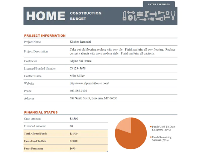 If you’re planning to remodel your house, you’d be foolish not to use this free home remodel budget template. With this, you’ll have a much better idea of what this undertaking is truly going to cost you.
23. Party planning template
Parties can also increase your spending for the month. Let this party planning template make sure your party stays within your budget.
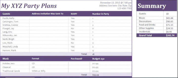
Purchasing a house is another important milestone that can quickly spiral out of your budget and control.
Fortunately, the templates in our next section will help alleviate some of the financial stress that comes with such a major purchase.
Buying a house
24. Home expense calculator template
 Your first step in the home buying process, even before you go house hunting, is to see how much home you can really afford. This home expense calculator will give you the truth.
25. Home buying checklist template
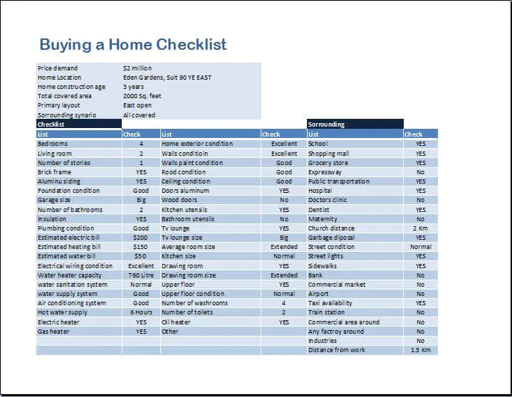 Once you have that all figured out, you’re ready for the fun stuff: deciding what you’d like in a house. This home buying checklist gives you a list of features to choose from so you can narrow down the type of house you’re looking for.
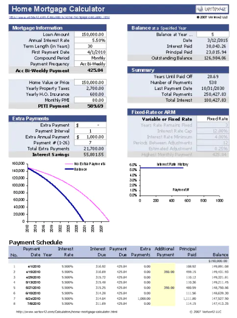
26. Mortgage calculator template
But before you decide to put in an offer on the house of your dreams, use this mortgage calculator template to see if your mortgage payments are something you can even afford.
Templates can also be helpful when you’re trying to lose or maintain your current weight. I’ll show you two great ones to use for this next.
Personal weight loss
27. Weight loss tracker template
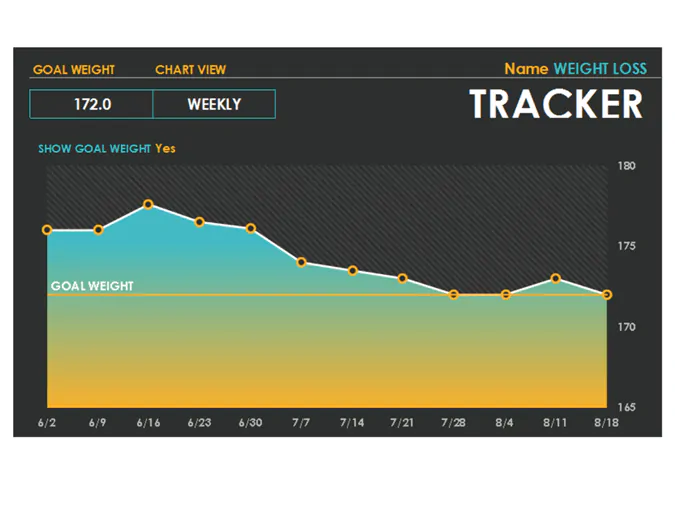 This free weight loss tracker helps you chart your weight loss journey so you can marvel at how much you’ve accomplished.
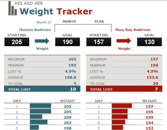
28. Couple weight loss tracker template
To add to that, grab a partner or spouse and track both of your weight loss journeys with this weight loss template. You can motivate each other to succeed.
Up next, let’s talk about the best Excel templates for managing your business.
Business management
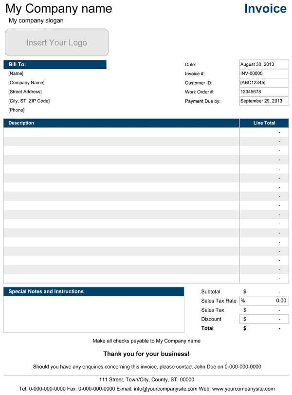
29. Basic invoice template
 When you need to create a simple invoice in order to receive payment from your customer, use this free template.
30. Service invoice template
 For service-based businesses, this invoice template has everything you need. You can explain what each charge is and describe the services performed neatly and easily.
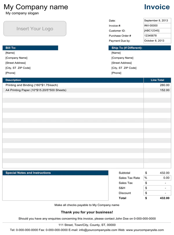
31. Sales invoice template
 If you’re collecting orders from customers, this sales invoice template has your name on it. With this, you’ll be able to track orders and clearly explain to customers exactly what they’re receiving with their purchase.
32. Account statement template
 As your month progresses, you can track your sales orders from customers using this free template to make sure you’re hitting your targets each time.
33. Packing slip template
 If you’re shipping goods to customers, use this packing slip template to show your customers a breakdown of their order.
34. Price quote template
 Anytime you need to send a customer a price quote, reach for this template and you’ll have a professional one to send over ASAP.
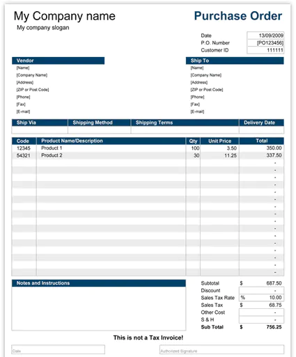
35. Purchase order template
Once your customer decides to accept your price quote, you can then create a purchase order thanks to this template.
36. Sales receipt template
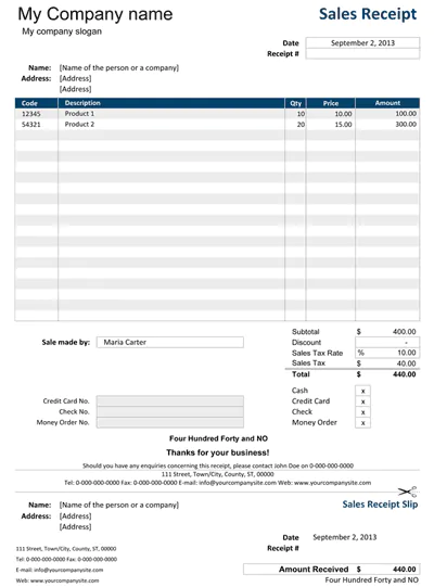 To send a simple sales receipt to your customers, use this free template.
37. Rent receipts template
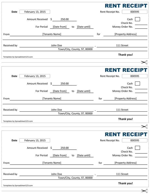 If you’re renting your home or business to a tenant, use these rent receipts to keep things organized. Come tax time, you won’t have to worry about finding the rent paper trail they’ll be asking for.
38. Home office expense tracking template
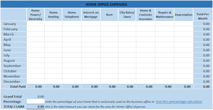 Solopreneurs working from home will want to use this home office expense tracker to double check that you’re making the most out of your eligible tax deductions.
39. Computer repair invoice template
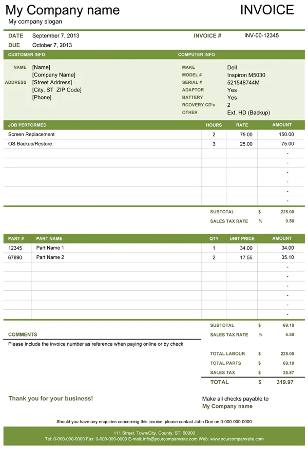 And if you happen to be in the computer repair business, use this free invoice template instead of the generic one so you can come across as professional and organized.
40. Time card template
 Keeping track of your employee time sheets should be a top priority for any manager. This free time card template does that in less time. Simply have your employees “clock in” each day using this sheet and at the end of the week, you’ll have everything you need to run payroll.
41. Weekly timesheet template
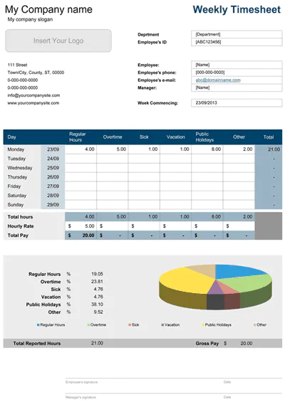 Once you have your employees’ daily log all set, you can then transfer that information to this weekly timesheet template to get a better view of their hours for the month.
42. Weekly timesheet with breaks template
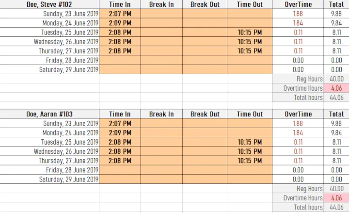 This weekly timesheet also includes breaks in it so you can get a more accurate picture of how many hours your employees are working each week. You can view a simple summary of both regular and overtime hours in the ‘Summary Timesheet’ tab.
43. Free payroll calculator template
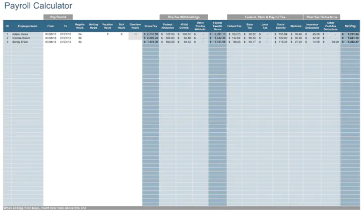 Before you run payroll, use this free payroll calculator to calculate your employee’s gross pay.
44. Proft and loss statement template
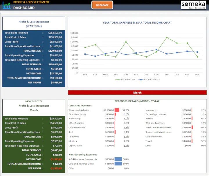 Finally, you can use this profit and loss template to track income statements, profits, revenues, and costs with an easy-to-use dashboard.
Now that you have templates for the technical aspects of operating your business, let’s go over a few to use if you’re just starting out or want to take your business to the next level.
Business planning
45. Competitive analysis template
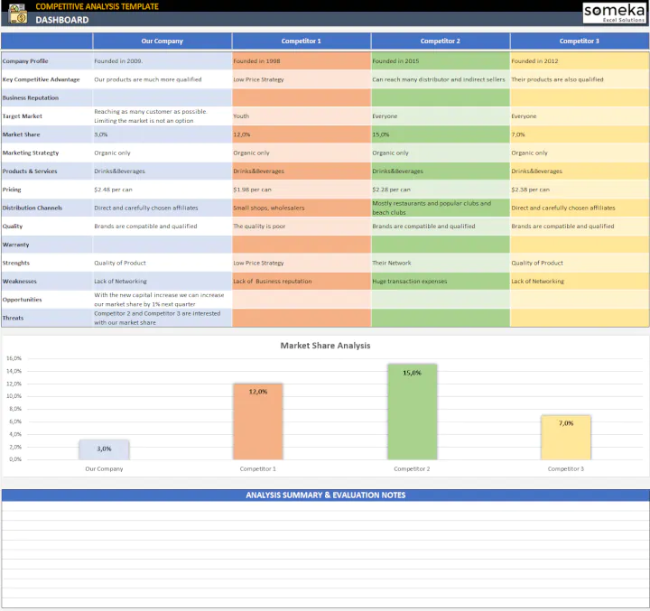 Before your idea becomes a business, it is vital to know where you stand in the competitive landscape. This handy competitive analysis template has sections for both qualitative and quantitative information on your competitors.
46. Startup business planning template
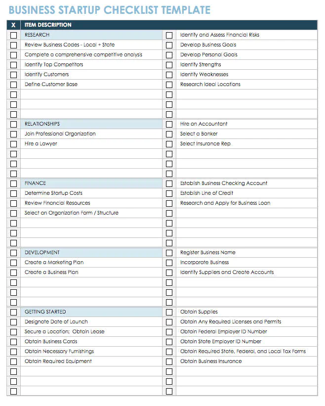 Every great business starts with two things: a good product and a solid business plan. While I can’t help you with the product itself, I can offer you this free Excel template which shows you everything you need to include in your business plan.
47. Financial plan projection template
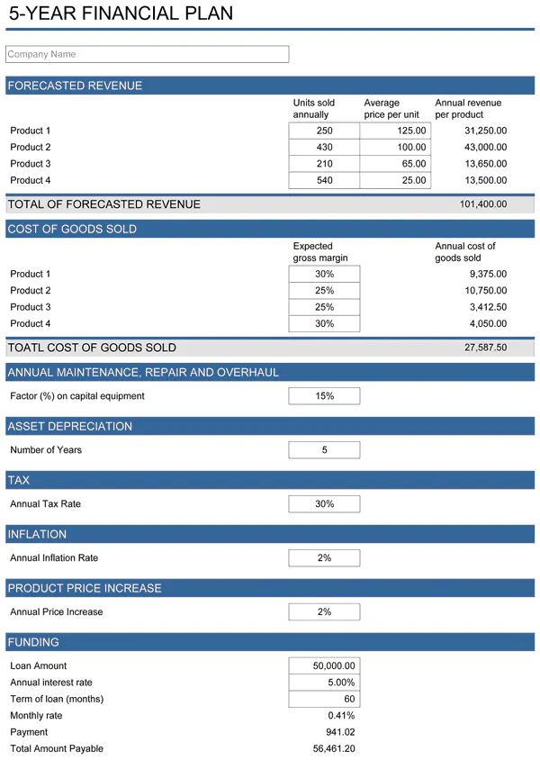 And if you’re stuck trying to figure out how to plan your finance, this template will be worth its weight in gold.
48. On-page SEO template
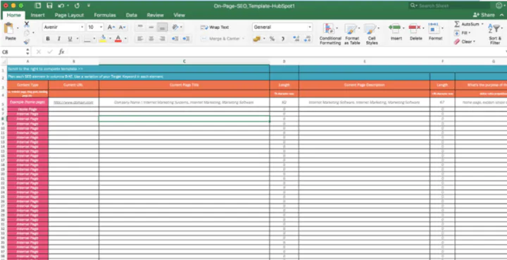 Before you launch your business’ website, or if you already have an existing one live, you should use this on-page SEO template to ensure your website is properly set up for search engines. This simple step can help you drive more leads to your website. If you’re looking to up your SEO game, check out these actionable SEO tips for startups.
49. Marketing calendar template
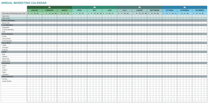 Once you have your business plan in place, conducted market research, and mapped out your customer’s journey, you’re ready to nail down your 12-month marketing plan. This template will make the task much less intimidating.
50. Marketing editorial calendar
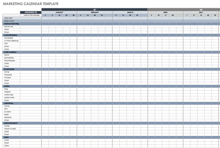 On top of your marketing plan, you’ll need an editorial calendar that outlines the type of content and social posts you’ll share with your audience. Use this free template to plan out the next few months of content for your business.
51. SWOT analysis template
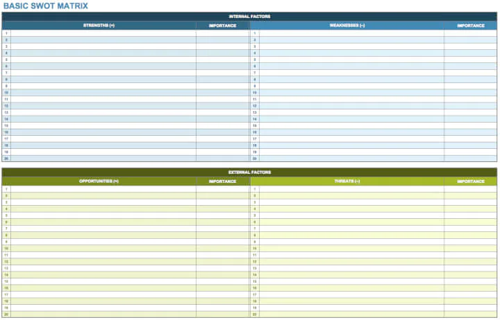 As your business grows, it’s essential that your team grows with it. To ensure your team is taking steps in the right direction, use this SWOT analysis for your business every few months.
52. Event planning template
 And when it comes time to celebrate your grand opening or a major milestone, be sure to take advantage of this event planning template so yours runs without a hiccup.
Don’t waste time creating your own templates, use these free Excel ones instead
You’re already busy enough, why add to your stress and overflowing to-do lists?
Instead of spending countless hours creating your own templates, use one of the free Excel templates on our list and you’ll make all the messy, overwhelming parts of your life that much easier.
Whether you’re starting a business or managing your personal finances, this list of 52 Excel templates has you covered.
Ready to become an Excel ninja? We got you – no matter where you are on the skill spectrum.
Check out our Basic and Advanced Excel course and level up today!
Level up your Excel skills
Become a certified Excel ninja with GoSkills bite-sized courses
Start free trial
Преобразование данных в таблицу
-
Введите данные, которые будут включены в таблицу.
-
Выделите любую ячейку с данными, а затем на вкладке Вставка нажмите кнопку Таблица.
-
Убедитесь в том, что выделены нужные ячейки или что ссылка на диапазон верна.

-
Убедитесь, что в таблице есть заглавные таблицы, и выберите ОК.
Добавление описательного имени таблицы
-
Выберите любую ячейку в таблице.
-
В >конструктора заменитеуниверсальное имя более осмысленным.
Применение специального макета
-
Щелкните в любом месте таблицы и перейдите на вкладку Конструктор.
-
Выберите нужные параметры, например Строка заголовка, Чередующиеся строки и Первый столбец.
-
Чтобы просмотреть все доступные стили таблиц, нажмите кнопку Дополнительные параметры.
-
В группе стилей Средний выберите стиль с контрастными цветами.
Увеличение размера шрифта
-
Выделите всю таблицу.
-
Перейдите на вкладку Главная и в поле Размер шрифта выберите значение не менее 12 пунктов.
Увеличение интервалов между строками
-
Выделите всю таблицу.
-
На вкладке Главная нажмите кнопку Формат и выберите пункт Высота строки.
-
Увеличьте высоту строк, например до 30 или 40, а затем нажмите кнопку ОК.
Изменение ширины столбцов в соответствии с содержимым ячеек
-
Выделить таблицу полностью.
-
Выберите Главная >формат >автооформат ширины столбца.
Ширина выбранных столбцов настраивается в том виде, в который в каждом столбце помещается самый длинный текст.
Выравнивание текста по левому краю
-
Выделите ячейки, столбцы или строки, содержимое которых нужно выровнять.
-
На вкладке Главная нажмите кнопку Выровнять по левому краю
.
 .
.Вам нужны дополнительные возможности?
Сделайте документы Excel доступными для людей с ограниченными возможностями
Скачивание бесплатных готовых шаблонов
Сохранение файла
Обучение работе с Excel
Обучение работе с Word
Обучение работе с PowerPoint
In general, any organised data is called a table. But in excel they are not. You need to format your data as a table on excel to get the benefits of tabled data. We will explore those beneficial features of Tables in Excel in this article.
How to Make Table in Excel?
Well, it’s easy to create a table in excel. Just select your data and press CTRL+T. Or
- Go to the home tab.
- Click on formate as table.
- Choose your favourite design.
And It is done. You have an Excel Table now.
Easy Formatting of Data Table
The first visible advantage of an excel table is striped formatting of data. This makes it easy to navigate through rows.

Change Table Designs Quickly
You can select from pre-installed designs for your dataset. You can also set your favourite design as default. Or create a custom new design for your tables.
Create Dynamic Pivot Tables
The pivot tables created with Excel Tables are dynamic. Whenever you add rows or columns to the table, the pivot table will expand its range automatically. It goes for the deletion of rows and columns too. It makes your pivot table more reliable and dynamic. You should learn how to make dynamic pivot tables anyway.
Create Dynamic Charts.
Yes, once you create your charts from an Excel Table, it is dynamic by itself. You don’t need to edit the chart after editing data in a table in excel. The range of chart will extend and shrink as the data in table extends or shrinks.
Dynamic Named Ranges
Each column of tables is converted into a named range. The heading name is the name of that range.
How to Name a Table in Excel?
You can easily rename the table.
- Select any cell in Table
- Go to design
- In the left corner, you can see the default name of the table. Click on it and write a suitable name for your table.
You can’t have two tables with the same names. This helps us in distinction among tables.
I named my table “Table1”, we will use this further in this article. So yeah guys keep following it.
Easy Writing Dynamic Formulas
So when you don’t use tables, to count “Central” in the region you would write it like, =COUNTIF(B2:B100,”Central”). You need to be specific about the range. It’s not readable to any other person. It will not expand when your data expands.
But not with Excel Tables. The same can be done with excel tables with more readable formulas. You can write:
=COUNTIF(table1[region],”Central”)
Now, this is very readable. Anyone can tell without looking at the data that we are counting Central in the region column of Table1.
This is dynamic too. You can add rows and columns to the table, this formula will return the correct answer always. You don’t need to change anything in the formula.
Easy Autofill of Formula in Columns
If you write a formula adjacent to the excel table, excel will make that column part of the table and will autofill that column with relative formulas. You don’t need to copy-paste it in the below cells.
Always Visible Headers without Row Freezing.
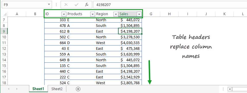
One common problem with the normal set of data is that the column headers vanish when you scroll down for data. Only column alphabets can be seen. You need to freeze the rows to make headers always visible. But not with Excel Tables.
When you scroll down, the headers of the table replace column alphabets. You can always see the headers on the top of the sheet.
Navigate to Table Easily from any Sheet
If you are using multiple sheets with thousands of multiple tables and forget where a particular table is. Finding that table will be hard-won.
Well, you can find a particular table easily in a workbook by writing its name on the name bar. Easy, isn’t it?
Easy SUBTOTAL Formula application
Excel Tables have the totals row by default to the bottom of the table. You can choose from a set of calculations to do on a column from SUBTOTAL function, like SUM, COUNT, AVERAGE, etc.
If the total row is not visible then press CTRL+SHIFT+T.
Get Structured Data
Yup! Like a database, the excel table is well structured. Every segment is named in a structured way. If the table is named as Table1 then you can select all data in a formula by writing =COUNTA(Table1).
If you want to select everything including headers and totals =COUNTA(Table1[#All])
To select the only headers, write Table1[#Headers].
To select only totals, write Table1[#Totals].
To select only data, write Table1[#Data].
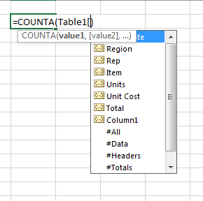
Similarly, all columns are structured. To select column fields, write Table1[columnName]. The list of available fields is displayed when you type “tablename[“ of the respective table.
Use Slicers With Tables
The slicers in excel can’t be used with normal data arrangement. They can be used with pivot tables and excel tables only. In fact, pivot tables are tables in itself. So yeah, you can add slicers to filter your table. Slicers give your data an elegant look. You can see all available options right in front of you. This is not the case with normal filters. You need to click on the drop-down to see the option.
To add a sliver to you table write follow these steps:
- Select any cell from the table
- Go to the Design tab
- Locate the Insert Slicer icon.
- Choose each range of which you want a Slicer to be inserted
The slicers are on now.
Click on items from which you want to apply filters. Like you do on web applications.
Useful, isn’t it?
You can clear all filters by clicking on the cross button on the slicer.
If you want to remove slicer. Select it and hit the delete button.
Run MS Queries From Closed Sheets
When you have master data that is stored in the form of a table and you often query the same thing from that master data, you open each time. But this can be avoided. You can get filtered data in another workbook without opening the master file. You can use Excel Queries. This only works with Excel Tables.
If you go to the Data tab, you will see an option, Get External Data. In the menu, you will see an option “From Microsoft Query”. This helps you Dynamically Filter Data from One Workbook to Another in Microsoft Excel.
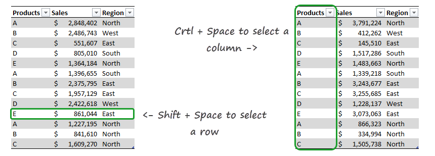
Enhanced Excel Shortcuts
In a normal data table, when you want to select the whole row containing data, you go to the first cell and then you use CTRL+SHIFT+ Right Arrow Key. If you try SHIFT+Space, it selects the whole row of the sheet, not the data table. But in Excel Table when you press SHIFT+Space, it only selects the row in the table. Your cursor can be anywhere in table row.
How To Convert a Table to Ranges?
One drawback of the table is that it takes too much of memory. If your data is small, it’s fantastic to use, but when your data expands to thousands of rows it gets slow. At that time you might want to get rid of the table.
To get rid of the Table, follow these steps:
- Select any cell from the table
- Goto Design tab
- Click on Convert to Range
- Excel will once confirm it from you. Hit the yes button.

As soon as you give your confirmation of converting the table to the range, the very design tab will vanish. It will not affect any formulas or dependant pivot tables. Everything will work fine. It’s just that you will not have features from the table. And yes, Slicers will go to.
Formating will not go.
Whenever you convert the table to the range, you might expect formatting of the table to be gone. But it won’t. It is suggested to clear the formating first than convert to ranges. Otherwise, you will have to clear it manually.
So yeah guys, this is all I can think about the Excel Tables right now. If you know any other benefits of Tables in Excel then let me know in the comments section below.
Related Articles:
Pivot Table
Dynamic Pivot Table
Sum by Groups in The Excel Table
Use VLOOKUP from Two or More Lookup Tables
Count table rows & columns in Excel
Show hide field header in pivot table
Popular Articles:
How to use the VLOOKUP Function in Excel
How to use the COUNTIF function in Excel
How to use the SUMIF Function in Excel
What are Excel Tables?
Tables in Excel helps group related data into one or more rows and/or columns. Once a table is created, Excel assigns a unique name to the columns and the table itself. Such names are used as structured references, which make it easy to apply Excel formulas. Therefore, tables eliminate the need to create named ranges in Excel.
For example, the following image shows a usual data range on the left side and an Excel table on the right side. Notice the alternately colored excel rowsThe two different methods to add colour to alternative rows are adding alternative row colour using Excel table styles or highlighting alternative rows using the Excel conditional formatting option.read more and structured references (in cell J2) of the latter.
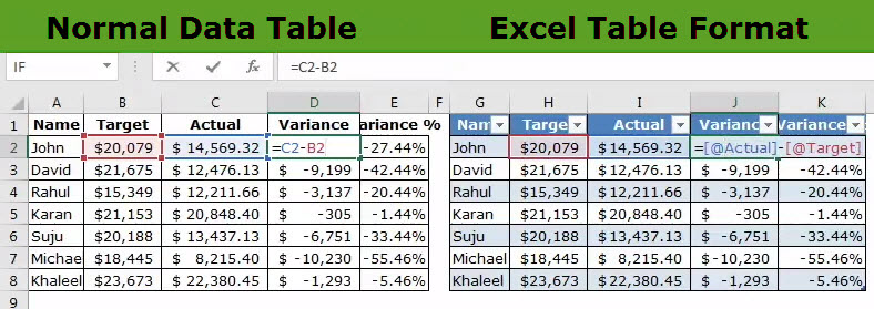
The purpose of creating tables is to make the data manageable, organized, and fit for analysis. Apart from structured references, tables offer several benefits like quick sorting and filtering, automatic expansion, easy formatting, readable formulas, and so on. Tables are extremely helpful when working with large databases.
Table of contents
- What are Excel Tables?
- How to Create Tables in Excel?
- How to Customize Tables in Excel?
- #1–Change the Name of the Table
- #2–Change the Color of the Table
- What are the Advantages of Creating Tables in Excel?
- #1–Creates Structured References Automatically
- #2–Is Dynamic in Nature
- #3–Makes it Easy to Work With PivotTables
- #4–Freezes Header Row Automatically
- #5–Helps add a Total Row Containing Functions
- #6–Eases Restoring to Usual Data Range Without Losing the Table Style
- #7–Helps add Slicers for Filtering Data
- #8–Assists in Creating Reports in Power BI
- How to Turn off Structured References in Excel?
- Frequently Asked Questions
- Recommended Articles
How to Create Tables in Excel?
You can download this Excel Tables Template here – Excel Tables Template
The steps to create a table in Excel are listed as follows:
- Ensure that the raw data does not contain any empty rows and/or columns. Further, each column should have a unique heading. If any two columns have the same headers, Excel automatically changes one of these headers once a table is created.
The raw data is shown in the following image.
Note: A column header should not contain any Excel formulas.

- Select any cell of the raw data and press the shortcut “Ctrl+T.” Both keys of the shortcut should be pressed together.
Note: Alternatively, after selecting a cell of the raw data, click “table” from the Insert tab of Excel. This option is in the “tables” group of the Excel ribbon.

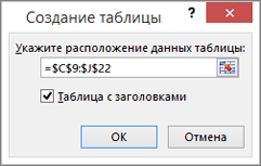
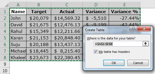
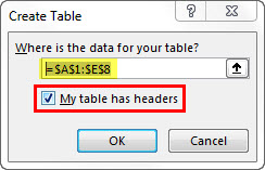
- The “create table” dialog box opens, as shown in the following image. Excel automatically selects the range for the table. Check whether this range is correct or not. If not, it can be edited.

- Select or deselect the checkbox of “my table has headers.” If selected, Excel will treat the content of the first row (row 1) as column headers.
In the preceding table, row 1 does contain column headers. So, we have selected the option “my table has headers.” Next, click “Ok.”

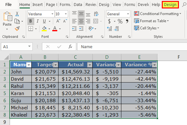
- An Excel table has been created. It is shown in the following image. Notice that the banded rows and filters (to the right of each column header) appear automatically.
Note: In Excel, banded rows are those in which color or shading is applied alternately.


How to Customize Tables in Excel?
A table can be customized by changing its name and/or the default color (or table style). Let us learn how this is done.
#1–Change the Name of the Table
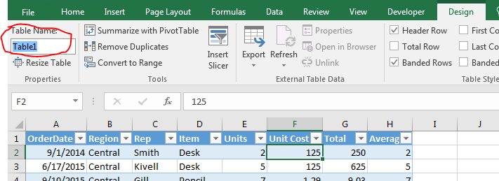
When a table is created, Excel assigns a default name like “table1,” “table2,” etc., depending on whether it is the first or the second table of the current workbook.
Working with such default names may become confusing, especially when there are lots of tables. So, the solution is to assign unique names to each table.
The steps for changing the name of the Excel table are listed as follows:
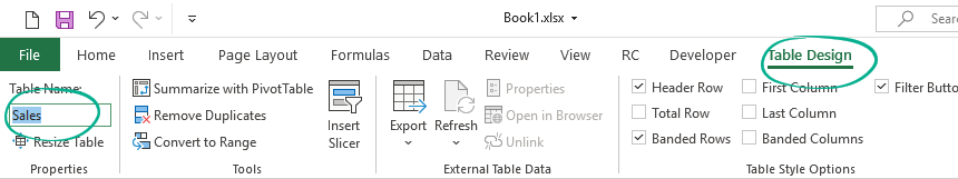
Step 1: Select the entire table. Once selected, the Design tab appears on the Excel ribbonRibbons in Excel 2016 are designed to help you easily locate the command you want to use. Ribbons are organized into logical groups called Tabs, each of which has its own set of functions.read more. This tab is shown within a red box in the following image.
Note: In place of the entire table, even if a single cell is selected, the Design tab will become visible.
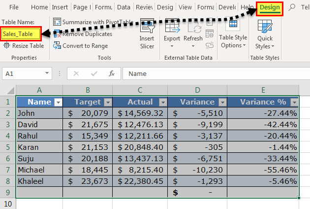
Step 2: In the Design tab, perform the following tasks:
- Click inside the box under “table name.” This box is displayed in the “properties” group at the leftmost side of the ribbon.
- Enter the desired name in this box.
- Press the “Enter” key.
Our table has been named “Sales_Table.” This is shown in the following image.
Rules Governing the Table Names
While naming a table, the following points should be considered:
- The name should always begin with a letter, a backslash () or an underscore (_).
- The name cannot be the single letter “r” (or “R”) or “c” (or “C”).
- The name should not consist of any spaces. Instead, one can use an underscore (_) or a period (.) to separate the words.
- The name can contain numbers, but cell references should be avoided.
- The name can contain a maximum of 255 characters.
- The name of the table should be unique. In case of a duplicate name, a message will be displayed saying that a unique name should be chosen.
Note: A name is said to be duplicate if two tables within the same workbook have the same names. Further, Excel does not distinguish between the uppercase and lowercase letters in the name of a table. So, the names “abc” or “ABC” are considered the same by Excel.
#2–Change the Color of the Table
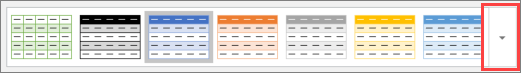
When a table is created, Excel assigns it a default color. To change the color of the table, its style needs to be changed. Excel displays a list of different table styles from which one can choose the desired option.
The steps to change the color (or style) of a table are listed as follows:
Step 1: Select either a cell of the table or the entire table. We have selected the latter. The Design tab becomes visible, as shown in the following image.

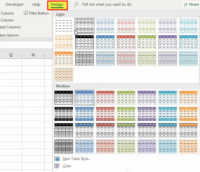
Step 2: Choose the desired color (or style) from the “table styles” group of the Design tab. To expand the list of table styles, click the “more” button displayed at the bottom right side. One can also click “new table style” to view more styles.
The following image shows the expanded list of table styles. Once the desired style is chosen, it will be applied to the entire table.
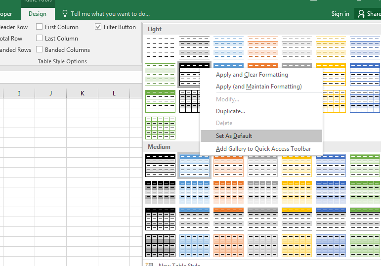
Note: The default table style of the workbook can be changed by the user. For making this change, perform the listed steps:
- Select the desired table style from the list of table styles.
- Right-click the selected table style and choose “set as default” from the context menu.
What are the Advantages of Creating Tables in Excel?
Let us discuss eight advantages of creating tables in Excel.
#1–Creates Structured References Automatically
An Excel table uses structured referencesIn Excel, structured references define data sets in columns by giving names instead of cell address. You may use the column name instead of the cell address in the formula; this makes work easier.read more for referencing one or more cells. This is in contrast with the direct cell addresses used in a normal data range. A structured reference is a combination of table and column names that are used in Excel formulasThe term «basic excel formula» refers to the general functions used in Microsoft Excel to do simple calculations such as addition, average, and comparison. SUM, COUNT, COUNTA, COUNTBLANK, AVERAGE, MIN Excel, MAX Excel, LEN Excel, TRIM Excel, IF Excel are the top ten excel formulas and functions.read more.
The major benefits of using structured references are listed as follows:
- They automatically update when new entries are added or deleted from the table.
- They are automatically created when one or more cells of the table are selected.
- They can be used both within and outside the table, thus making it easy to locate tables in a workbook.
- They are used to autofill the calculated columns. A calculated column is an additional column added to the existing Excel table. It uses a single formula that expands on its own in the remaining part of the column. This implies that when a formula is entered in one cell of a calculated column, it need not be dragged to the remaining cells of the column. Rather, the formula is automatically entered in all cells (called autofill), unlike a usual data range which requires one to drag the fill handleThe fill handle in Excel allows you to avoid copying and pasting each value into cells and instead use patterns to fill out the information. This tiny cross is a versatile tool in the Excel suite that can be used for data entry, data transformation, and many other applications.read more.
Example of point “d”: The range A2:B7 is an Excel table containing random numbers. To create column C as a calculated column, enter the SUM formula in cell C3, which adds the numbers of cells A3 and B3. Use structured references in this formula. Once the formula is entered, press the “Enter” key. The outcomes are stated as follows:
- The table (A2:B7) automatically expands to include column C.
- The range C4:C7 is automatically filled with the totals of each row of the table.
The preceding results will be obtained with both structured and regular references. This is because autofilling is a feature of Excel tables. However, with structured references, it is easy to read and understand the formula.
Note that if the user makes a change to the formula of the calculated column, the change is automatically replicated in the entire column.
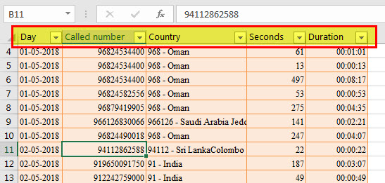
Example of structured references: In the following image, structured references have been used in the SUMIF formula. The “Calls_Table” is the name of the Excel table. “Day” and “duration” are the names of columns A and E respectively. The cell G2 is a direct cell referenceCell reference in excel is referring the other cells to a cell to use its values or properties. For instance, if we have data in cell A2 and want to use that in cell A1, use =A2 in cell A1, and this will copy the A2 value in A1.read more.
Note: In the following image, the black line pointing to cell G2 has been incorrectly placed. It should have pointed to “day,” which is the name of column A. So, please ignore the misplacement.

#2–Is Dynamic in Nature
Any new insertions to the cells below or to the right of the table are automatically included in the Excel table. This implies that the table expands to include such insertions. Likewise, the table contracts when one or more rows and/or columns are deleted from it. Due to automatic expansion and contraction, an Excel table is often considered a dynamic tableDynamic tables in Excel are ones in which the table automatically adjusts its size when a new value is inserted. It can be done in one of two ways: by using the offset function or by creating a data table from the table section.read more.
Expansion implies that the style, formatting, and formulas of the table are automatically applied to the new entries as well. This eliminates the need to format and edit the formulas of individual cells. By default, the formatting stays uniform throughout an Excel table.
Note that the formulas of the table are adjustable as they take into account structured references. In contrast, the formulas of a normal data range do not adjust with insertions or deletions of entries.
Note: To undo table expansion, press the keys “Ctrl+Z” together.
#3–Makes it Easy to Work With PivotTables
It is advised to create a PivotTableA Pivot Table is an Excel tool that allows you to extract data in a preferred format (dashboard/reports) from large data sets contained within a worksheet. It can summarize, sort, group, and reorganize data, as well as execute other complex calculations on it.read more from an Excel table. The major reasons the source data should be an Excel table are listed as follows:
- A PivotTable automatically updates with any changes in the source table. Since Excel tables are dynamic, the data range of the PivotTable also becomes dynamic.
- A single cell of the source table can be selected prior to inserting a PivotTable. In contrast, when the source data is a usual data range, the entire range (or dataset) needs to be selected prior to inserting a PivotTable.
For instance, in the following image, a single cell of the source table has been selected before clicking the “PivotTable” option from the Excel Insert tabIn excel “INSERT” tab plays an important role in analyzing the data. Like all the other tabs in the ribbon INSERT tab offers its own features and tools. Under Insert Tab we have several other groups including tables, illustration, add-ins, charts, Power map, sparklines, filters, etc.read more. Notice that in “table/range,” the name of the source table is reflected.

When one scrolls downwards in a worksheet, the table headers are visible at all times. This is because these headers are automatically fixed or frozen at their respective places.
Fixed headers prevent the user from going back to the top row (row 1) again and again. Such frozen headers can be seen within a red rectangle in the following image.
Notice that the user has scrolled downwards such that rows 4 to 13 are visible along with the header row.
Note: To see the frozen header row, ensure that a cell of the table is selected before scrolling.
#5–Helps add a Total Row Containing Functions
An Excel table shows various functions in the total row. For displaying this row, perform the following steps:
- Select any cell of the Excel table. The Design tab appears on the Excel ribbon.
- From the Design tab, select the checkbox of “total row” displayed in the “table style options” group.
The total row is added immediately below the Excel table. Select any cell of this row to see a drop-down arrow on the right side. When this arrow is clicked, a list containing functions appears, as shown in the following image.
Once a function is selected from the list, the respective formula is automatically entered and the output is shown in a cell of the total row.
Notice that row 9 of the following image is the total row. Further, if a function is selected in cell D9, the corresponding output will also be displayed in this cell. The formula will be visible in the formula bar of the worksheet.

#6–Eases Restoring to Usual Data Range Without Losing the Table Style
An Excel table can be quickly converted to a usual data range. This serves as a benefit when the user requires only the table style and not the functionality of the table. For such conversion, follow either of the listed steps:
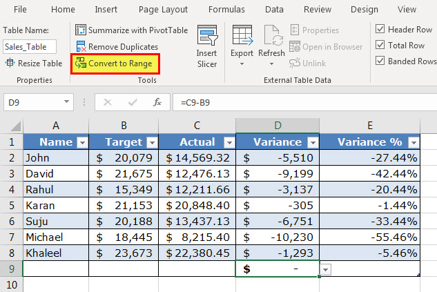
- Select any cell of the table. From the Design tab, click “convert to range” in the tools group.
- Select any cell of the table and right-click it. From the context menu, choose “table” followed by “convert to range.”
The “convert to range” feature of the first pointer is shown in the following image. Once an Excel table is converted to a usual data range, the existing structured references are replaced with the regular cell references. However, the data and formatting of the table are retained in the usual data range.
Note: The “convert to range” feature can be used only when the data to be converted is in the form of an Excel table.
#7–Helps add Slicers for Filtering Data
A slicer helps filter the data of an Excel table. It displays buttons that can be selected or deselected to indicate whether an item is included or excluded from the filter.
Slicers are available in Excel 2013 and the newer Excel versions. The steps to add a slicer to a table are listed as follows:
- Select either a cell within the table or the entire table.
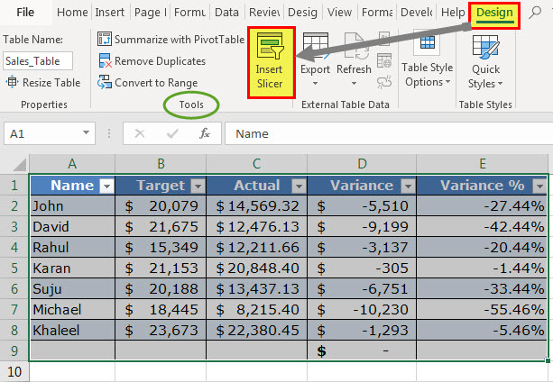
- From the Design tab, select “insert slicer” from the “tools” group.
- The “insert slicer” dialog box opens. Next, select the checkboxes of the columns for which the slicer needs to be created.
- Click “Ok.”
One can have a slicer for each column of the Excel table. Once slicers appear in the worksheet, they can be moved, resized, and formatted according to the requirement.
With a slicer, one can filter and view only particular items (or entries) of the table. To view multiple items of a column, press and hold the “Ctrl” key while selecting the items in the respective slicer.
The following image shows the “insert slicer” option of the Design tab.
Note 1: A slicer can also be added from the “filters” group of the Insert tab of Excel. Click “slicer” in this group and thereafter follow the steps “c” and “d” listed above.
Note 2: A slicer can be used only if the data is in the form of an Excel table.
#8–Assists in Creating Reports in Power BI
Excel tables serve as a source from which data is entered in the Power BI tool. Power BI is a business intelligence tool that helps convert unrelated sources of data into meaningful reports and dashboards. The process of creating reports works as follows:
- Create and upload Excel tables to Power BI.
- Create a report in Power BI by adding visualizations.
- Share the report with other Power BI users or office colleagues.
Excel tables are a preferred data source in Power BI due to the following reasons:
- They allow quick access to the tabular format of the dataset.
- They help ease comparisons within a dataset.
- They can be easily edited and organized prior to being uploaded in Power BI.
How to Turn off Structured References in Excel?
The steps to turn off structured references in Excel are listed as follows:
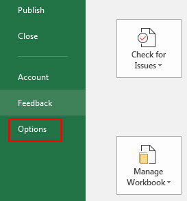
Step 1: Click the File tab of Excel. It is displayed within a red box in the following image.

Step 2: Select “options” shown in the following image.
Step 3: The “Excel options” dialog box opens. Click “formulas” appearing on the left side of the window. Deselect the checkbox of “use table names in formulas.” This is shown in the following image.
Next, click “Ok.” The structured references will be turned off in Excel.
Note: By changing this setting, the structured references used in the existing formulas of the Excel table are not removed. However, the new formulas applied to the table will contain regular cell references instead of structured references. If regular cell references are required in existing formulas too, they will have to be edited manually.
Further, whether the structured references are turned on or off, the changed setting will be applied to all workbooks that the user is working on.

Frequently Asked Questions
1. What are Excel tables and how are they created?
An Excel table displays the data in a tabulated format. Every column should have unique headers (or names) according to the kind of data they contain. Such headers are placed in the top row of the table. The table may or may not be named by the user.
If the columns and table are not named by the user, Excel assigns default names to both of them. These names are used as structured references in all formulas applied within or outside the table (that contain a table reference).
To create a table in Excel, select any cell of the dataset and press the keys “Ctrl+T” or “Ctrl+L.”
2. How to join two tables in Excel?
Two tables that have a common column can be joined with the help of the VLOOKUP function of Excel. The formula is stated as follows:
“=VLOOKUP(lookup_value,entire_lookup_table,return_column,FALSE)”
For instance, the first table is named “table1” and the second table is named “table2.” To pull the data of a single column of “table2” in “table1,” enter the following formula:
“=VLOOKUP($A2,table2,3,FALSE)”
This formula looks up the value of cell A2 in “table2.” It returns an exact match from the third column of “table2.”
One can use either regular or structured references in the given formula. By selecting the cell of the “lookup_value” and the range of the “entire_lookup_table,” Excel will automatically enter structured references in the VLOOKUP formula.
Note 1: Enter the given formula in the first cell to the immediate right of the first table. Once entered, press the “Enter” key. The Excel table expands to include the new column. Consequently, the outputs of the entire column are displayed in the first table.
Note 2: For the given formula to work, the column containing the “lookup_value” should be common to both tables. Moreover, the lookup column (containing the “lookup_value”) should be the leftmost column of the second table. The return column (containing the value to be returned) of the second table should be to the right of the lookup column.
3. When should Excel tables be used and how to locate them in a workbook?
Excel tables should be used in the following situations:
• To arrange data in a tabular format
• To facilitate comparisons of data values
• To improve the readability of the dataset
• To ease data analysis and eventually assist in decision-making
To locate tables in a workbook, click the downward arrow appearing on the right side of the name box. It shows the names of all the tables of the workbook. Clicking on any of these names will select that particular table.
Recommended Articles
This has been a guide to tables in Excel. Here, we explain how to create/insert/customize Excel tables along with examples and advantages. You may also look at these useful functions of Excel–
- Delete Pivot Table ExcelTo delete a pivot table in Excel, you must first select it. Then go to the Analyze menu tab under the Design and Analyze menu tabs and select actions. Then, from the Select option’s drop-down option, select Entire Pivot Table to delete it.read more
- Refresh Pivot Table in ExcelTo refresh pivot tables, you may use the following methods — refresh pivot table by changing data source, refresh pivot table using right click option, auto-refresh pivot table using VBA Code, refresh pivot table when you open the workbook.read more
- Data Table in Excel
- Excel Merge Tables We can use a number of different methods to merge tables in Excel, including the VLOOKUP function, the INDEX function, and the MATCH function.read more
Use Excel Tables to simplify your work! Learn how to create dynamic ranges, easy-to-read formulas using a table. In this tutorial, we’ll explain how to add new data to a range or how to manage Tables. Keep your formulas ready for auditing!
This guide provides useful tricks and examples.
- Fundamentals of Excel Tables
- Creating an Excel Table is Easy
- Add a name for a Table
- The Parts of a Table
- Navigating between Tables
- Table related Shortcuts
- Working with Tables
- Moving Excel Tables
- Swapping rows or columns in the table
- Keep Table headers always on the top
- Expand your Table easily
- Show Totals (Sum, Count, Min, Max) without using formulas
- Resize an Excel Table
- Table Formatting
- Change table formatting quickly
- Choose your Table style
- Tables and Data sources
- Quick Analysis works with Excel Tables
- Use a Table as a pivot table source
- Build dynamic charts using Tables
- Insert a new slicer into a table
- Convert Excel Tables to a normal range back
Fundamentals of Excel Tables
In this section, we’ll start with the basics.
Creating an Excel Table is Easy
How to create an Excel table?
- Select the range which contains data.
- Use the insert Table keyboard shortcut, Control + T
- If your table has headers, select the ‘My Table has headers’ checkbox.
- Click OK, and Excel will create a new table.
If you are in a hurry, Excel Tables is yours! On the right side of the picture, you’ll see banded rows.
Rename a Table
When you create a new Excel Table, Excel will assign a custom name, like Table1. You have to rename it and add a short, user-friendly name like ‘Sales.’
Important: Each table must have a unique name that contains letters, numbers, or the underscore character (for example, using spaces or special characters between words is not allowed.
To change the default name, select your table and locate the Table Design Tab. Jump to the Table Name > Properties section. Add a new name and press Enter.
The Parts of a Table
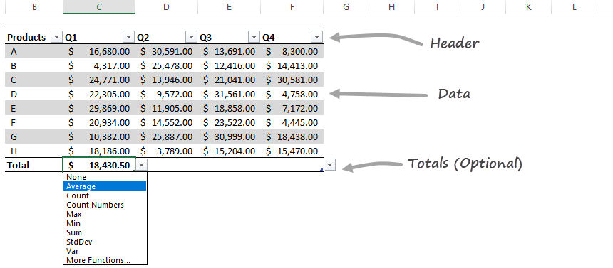
All Excel Tables have two required and one optional part.
The Column Header Row is the first row of the table. It contains identifiers, for example, ‘Product,’ ‘Order Date,’ and so on.
The body is the main data set.
Optional: you can switch an additional (Totals) row using the ‘Ctrl + Shift + T‘ shortcut.
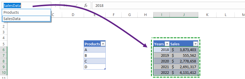
Navigating between Tables
If you want to find your table quickly, locate the Name Box and use the drop-down menu in the top-left area of your workbook. Choose the table name, and what you want to activate. The range will be highlighted.
What if your table is located in a different tab? Excel will jump to the selected table.
If you have tabular data, you can easily convert it to an Excel Table.
If you select a simple cell in the table, you can select the actual row using the ‘Shift + Space’ command. To select rows, use the ‘Control + Space’ keyboard shortcut.
Working with Tables
Moving Excel Tables
The easiest way to move a table to a new location is using a drag and drop method with a mouse.
In the example, we’ve just selected the original table then moved it to the K4:N13 range.
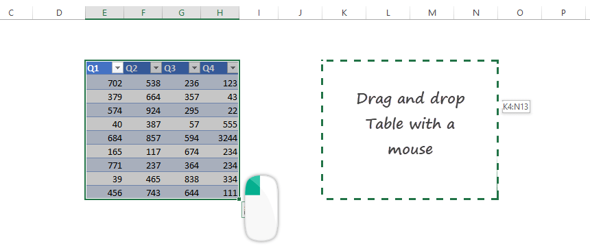
Tip: This is the fastest way to move tables to a new location. The method works only on the same sheet!
Swapping rows or columns in the table
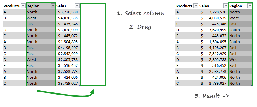
It can frequently happen that you want to change the table structure or swap rows or columns. As first, select the table row or a table column. Make sure that the header row is selected. Drag the selected range and drop to a new area.
Excel will swap the given rows or columns. The method is safe because Excel will not overwrite the existing data.
Excel Tables work simply. Are you working with large data sets? No problem! You can scroll down without any trouble. The table header will stay on the top. It’s not necessary to use the good old Freeze Top Rows function.
You can find it under the Freeze Panes group.
Expand your Table easily
In some cases, you need to insert rows or columns into an Excel Table. We’ll show you how to do that. The Excel Table is a dynamic range; it will resize even if you add or delete rows or columns.
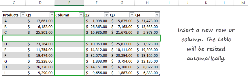
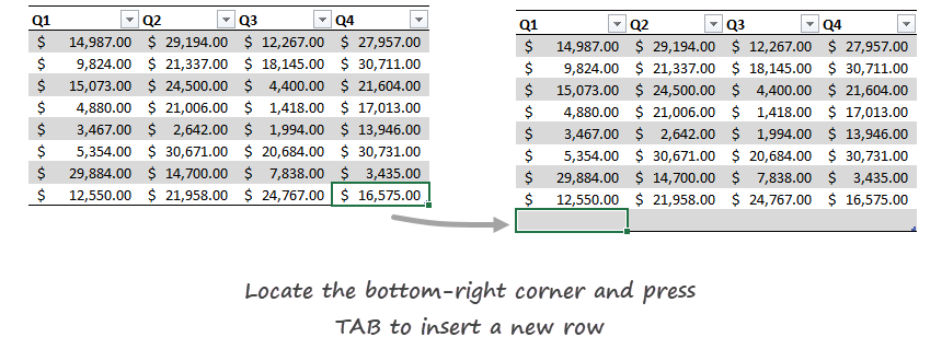
To add a new row, select the bottom-right cell in the range, in this example, cell F11. Press the Tab button; a new row appears, and the table structure remains.
It’s not necessary to select the range and add a new name for a range again.
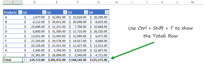
Show Totals (Sum, Count, Min, Max) without using formulas
With the help of tables, it’s easy to show dynamic Totals. Use your preferred formulas, like SUM, COUNT, AVERAGE, MIN, and MAX. Good to know that you don’t have to enter these formulas manually. Great!
You have a filtered Excel table on the left side and a regular table on the right side in the picture below. Use the ‘Control + Shift + T‘ shortcut to display the additional row under the table.
Resize an Excel Table
In the example below, you’ll learn how to change the table size using the ‘Resize Table’ command. This function is yours if you need to prepare a table for – for example – 500 rows.
To resize a table, select the new data range for your table. Click the OK button.
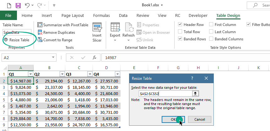
Note: The table headers must remain in the same row, and the resulting table range must overlap the original table range.
Or you can use the classic resize on the fly technic too. Select the small green triangle keeping the left mouse button pressed.
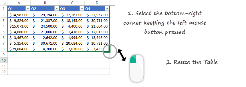
Table Formatting
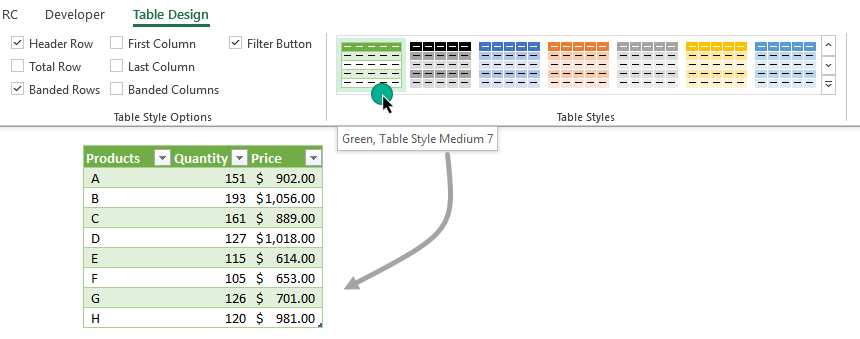
Change table formatting quickly
When you create a new table, it has a default formatting style. To override the displayed theme select a cell in the range. Choose the Table design tab on the ribbon and locate the Table Styles Group.
Click your preferred style, and the new theme will appear with a single click.
If you want to use the classic style without formatting, select the table and choose the default style by clicking on the top-left corner of the table style previews. The name of the first style is ‘None.’
Choose your Table style
You can choose a default table style. What is the default style? Start Excel and create your first table. Excel assigns a built-in style to the table.
Select the style that you want to apply to all new tables in the future. Right-click on the Table preview and click on the ‘Set as default’ option.
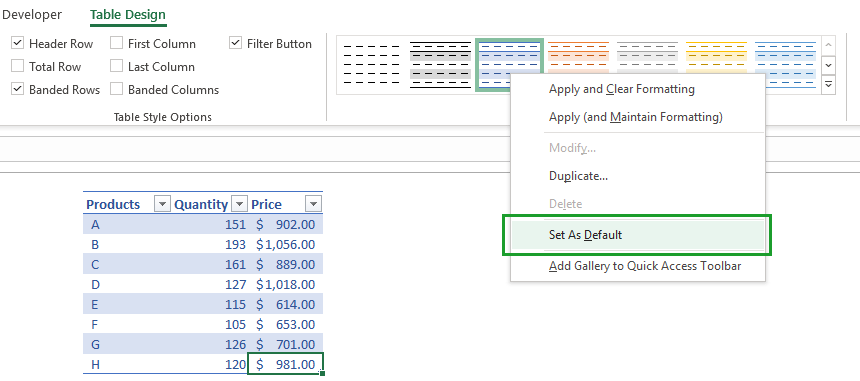
Learn more on how to remove table formatting in Excel.
Tables and Data Sources
Quick Analysis works with Excel Tables
Everyone knows that the Quick Analysis Tool is a great function in Excel. Create your table first. After that, click Control + Q to create a floating row like in the picture below:
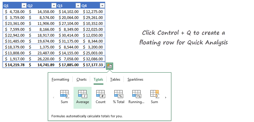
Apply various methods to analyze your data. Use conditional formatting, create chars, or calculate Totals, among others. If you need more power, use conditional formatting.
Use a Table as a pivot table source
Is it possible to use an Excel table as a pivot table source? Absolutely.
As we mentioned before, the Pivot table will track the changes in the table. If you add new data to the range, the pivot table will refresh automatically.
Go to the Insert tab. Insert a new pivot table.
A new window appears. Select the data that you want to analyze.
Finally, click OK.
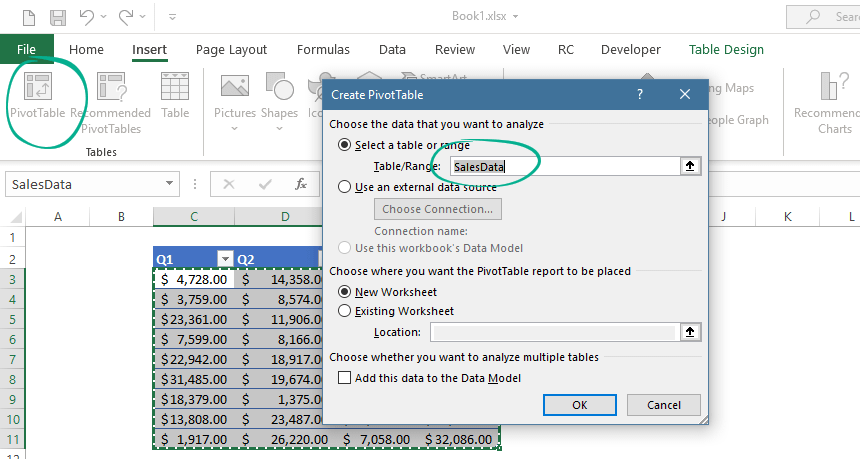
Build dynamic charts using Excel Tables
In our latest article, we’ve just talked about dynamic charts.
If you update your data frequently (adding rows or columns), tables are great for these purposes. Put your fresh data into the table, and the chart will refresh using the entered values.
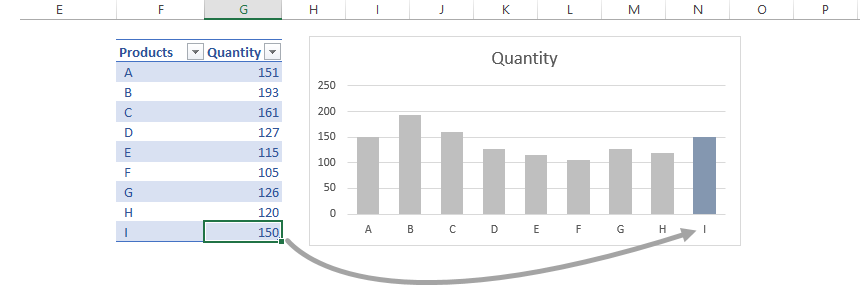
Insert a new slicer into a table
Good to know that all Excel Tables are slicer-ready? What does that mean in practice? Slicers are special filters. With its help, you can filter data quickly in various ways.
To add a new slicer:
- Select the table
- Locate the Table Design tab on the ribbon
- Locate the Tools group and Click the Insert Slicer button.
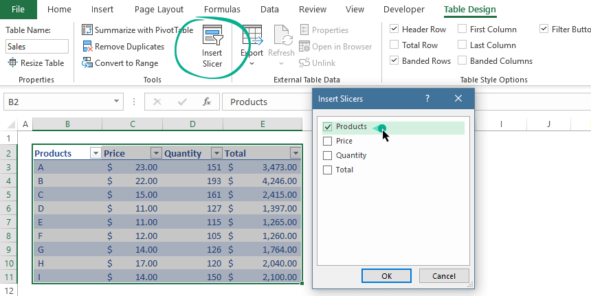
In the example below, now we have a slicer for Products:
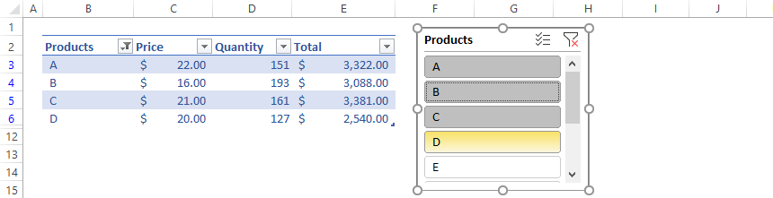
Convert Excel Tables to a normal range back
Tables are useful, but sometimes you need to work with normal ranges. To convert an Excel Table into a range back, do the following steps.
- Select the Table
- Remove the formatting style (choose the ‘None’ table style)
- Click on the Table Tools Tab
- Apply the ‘Convert to Range’ commands.
Note: Step 2 is necessary; otherwise, the formatting styles remain.
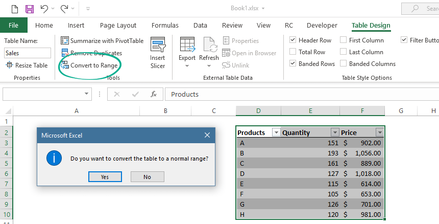
Conclusion
Excel Tables are versatile tools. With its help, you can speed up your daily tasks.
You May Also Like the Following Excel Tutorials:
- Creating an Excel Dashboard – The Ultimate Guide
- Structured references
I’m want to start using Excel Tables when building my spreadsheets. But first it’s instructive for me to explain how I think about “unofficial” tables or data tables as I like to call them.
How I Think About Tables
A data table is just a range of data, or a region of data that Excel recognizes if you were to use the keyboard shortcut Ctrl+Shift+*.
There are headings in the top row, which I refer to as column headings or data fields. Date, Shift, Machine, and Total Hours are all examples. The Date column has dates in it, and only dates. The Total Hours field has only hours data.
Each row of the data table represents one record. For instance, think about customers. A customer record would contain name, address, city, state, zip, phone number, etc.
My Initial Table Design
The data table I want to design is for a manufacturing facility. We want to record data for each machine by shift. This is common when machine logs are used to collect transactional data throughout the shift. The machine logs are summarized at the end of each shift and it’s this data we want to input into our spreadsheet or data table.
What’s not obvious here is what data fields are collected for input. Suffice to say that the reports have already been designed for key indicators of performance and waste, the calculations traced back to their lowest common denominator or required data field, and that’s what we’re going to collect.
My Table Inputs
I started the data table in row 4 to keep the top area clear for any global input fields and controls for the user. The data fields in the header row were entered and cells formatted: bold, center, word wrap, column widths. I haven’t gone with any background colors in the header row just yet because I’m waiting to see how the Table formatting will turn out.
The header row or data fields are: Date, Shift, Machine, Number Setups, Setup Hours, Run Hours, Down Hours, Total Hours, Net Product, Waste Setup, Waste Run, Gross Product.

I’ve entered the first row of data for a machine on shift one. My next task was to format the data. I used the default Date format for the US, m/d/yyyy, centered the Shift number and Number of Setups. The Hours fields are all formatted to one decimal number. And finally the Product and Waste fields have a number formatting with comma and zero decimal.
One Reason Regular Data Tables Fail
And now the moment where an unofficial Table fails miserably. When the second record gets entered the formatting is not the same. In fact check out the data in the second row. Not good. Not the same. (The Date really bothers me.)

Convert a Data Table to an “Official” Excel Table
Since I have the formatting set in the first row I’ll delete the second row before converting to a Table. I select a cell inside the table, then choose Insert > Table.

In Excel for Mac choose Tables > New > Insert Table with Headers.

Since Excel has recognized the correct range AND knows that my table has headers, I click OK.

Then as I’ve mentioned before, the first thing I do is remove the filter headings by choosing Data > Filter. Then I reset my column widths and re-enter the second row of data.

Now comes the whole point of this article. An Excel Table remembers the formatting for each data field or column of data.
There are other things that a Table “remembers” as you extend the data, but that will have to wait until next time.
![]()